SU(3) vortex-like configurations in the maximal center gauge FTUAM-99-24

Abstract

A new algorithm for fixing the gauge to (direct) maximal center gauge in SU(N) lattice gauge theory is presented. We check how this method works on SU(3) configurations which are vortex-like, and show how these configurations look like when center projected.

1 Introduction.

The maximal center gauge is widely used to study low energy phenomena such as the confinement property or the breaking of the chiral symmetry, as can be seen in a set of recent works [1, 2, 3, 4, 5, 6, 7, 8, 9] and also in these proceedings. Nevertheless, at least to our knowlegde, there was no efficient method of direct gauge fixing to maximal center gauge in SU(N) lattice gauge theory for values $N>2$. This is the motivation of the first part of this work in which we present a new algorithm of direct center gauge fixing to maximal center gauge. We apply this new method to previously prepared SU(3) vortex-like configurations. Our purpose in the second part of this work is to know how these configurations look like in the maximal center gauge, and therefore, whether these solutions have the properties described in references [1, 2, 3, 4, 5, 6, 7, 8, 9] for a confining object. For a more detailed description of our results see reference [10].

2 The method.

The maximal center gauge in SU(N) lattice gauge theory is defined as the gauge which brings link variables $U$ as close as possible to elements of the center $Z_{N}=\left\{e^{2\pi mi/N}1\!\!1\right.$ , $\left.m=0,...,N-1\right\}$. This can be achieved by maximizing the following quantity:

$$R=\frac{1}{N_{site}N_{dim}N^{2}}\sum_{n,\mu}\mid\mbox{Tr}\;U_{\mu}(n)\mid^{2}$$ (1)

where $N_{site}$ is the number of sites in the lattice and $N_{dim}$ the number of dimensions ($R$ satisfies $|R|\!\leq\!1$). Our procedure is based on a local update of $R$. We maximize this quantity respect to a gauge transformation $G(n)$ defined at the lattice point $n$. We build the SU(N) matrix $G(n)$ from a SU(2) matrix $g(n)$ as in the Cabbibo-Marinari-Okawa method. Doing the update in this way the problem is reduced to finding the maximum of a quadratic form, and this can be done using standard methods (see [10] for details). Once we obtain the SU(2) matrix $g(n)$ maximizing $R$, we update the $U_{\mu}$ variables touching the site $n$: $U_{\mu}(n)\rightarrow G(n)U_{\mu}(n)$ and $U_{\mu}(n-\hat{\mu})\rightarrow U_{\mu}(n-\hat{\mu})G^{\dagger}(n)$. We repeat this procedure over the $N(N-1)/2$ SU(2) subgroups of SU(N) and over all lattice points. When the whole lattice is covered once we say we have performed one center gauge fixing sweep. We make a number of center gauge fixing sweeps on a lattice configuration and stop the procedure when the quantity $R$ is stable within a given precision ($10^{-8}$ in this work).

3 The vortex solution.

Following the same methods used in [11] for the SU(2) group, we built a SU(3) Yang-Mills configuration which has the following features:

• It is a solution of the SU(3) Yang-Mills classical equations in $R^{4}$.

• It is constructed from $R^{2}\times T^{2}$ solutions of the SU(3) Yang-Mills classical equations by glueing to themselves the two periodic directions ($R^{2}\times T^{2}$ is considered the limit of $T^{4}$ with two periods much larger than the other two).

• The $R^{2}\times T^{2}$ building block satisfies non-orthogonal twisted boundary conditions, is (anti)self-dual and has minimal action $S=8\pi^{2}/3$. The crucial point for this building block to have vortex-like properties is that the twist in the small plane must be non trivial.

We isolate the $R^{2}\times T^{2}$ building block using the lattice aproach. Working on lattices of sizes $N_{l}\!\times\!N_{l}\!\times\!N_{s}\!\times\!N_{s}$ (directions $t,x,y,z$ respectively and $N_{l}\!>>\!N_{s}$) and imposing twisted boundary conditions given by the twist vectors $\vec{k}\!=\!\vec{m}\!=\!(1,0,0)$ we isolate SU(3) configurations with topological charge $Q\!=\!-1/3$ and minimal action $S=8\pi^{2}/3$ using a standard cooling algorithm. The lattice sizes used are $N_{s}=4,5,6$ and $N_{l}=6\times N_{s}$, and we obtain configurations with action $S/(8\pi^{2}/3)=0.92219,0.95015$, $0.96536$ respectively. We fix the length in the small directions equal to $1$ and then the lattice spacing is $a=1/N_{s}$.

4 Properties of the solution

A) From the field strength ${\bf F}_{\mu\nu}$, obtained using the clover average of $1\times 1$ plaquettes, we calculate the quantity ${\cal E}_{\mu\nu}(x_{\mu},x_{\nu})$, the integral of the action density in two directions, defined as,

$${\cal E}_{\mu\nu}(x_{\mu},x_{\nu})=\int d^{2}x_{\alpha\neq\mu,\nu}\hskip 5.69046pt\frac{1}{2}{\rm Tr}\left({\bf F}_{\rho\sigma}{\bf F}_{\rho\sigma}\right)$$ (2)

and obtain the following results:

• Localized in the $xt$ plane as shown in the plot of ${\cal E}_{xt}(x,t)$ included in figure 1.

• Localized in the $x$ direction and almost flat in the $y$ direction as shown in the plot of ${\cal E}_{xy}(x,y)$ included in figure 1. In this case we repeat six times the y direction to obtain a box size equal to the one used in the figure for ${\cal E}_{xt}(x,t)$. Identical figures are obtained changing $x\rightarrow t$ and $y\rightarrow z$.

• Almost flat in the $y,z$ directions as shown in the plot of ${\cal E}_{yz}(y,z)$ included in figure 1. We repeat six times both directions to obtain a box size equal to the one used for ${\cal E}_{xt}(x,t)$.

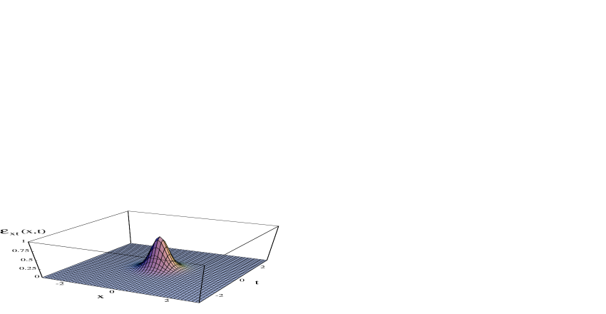
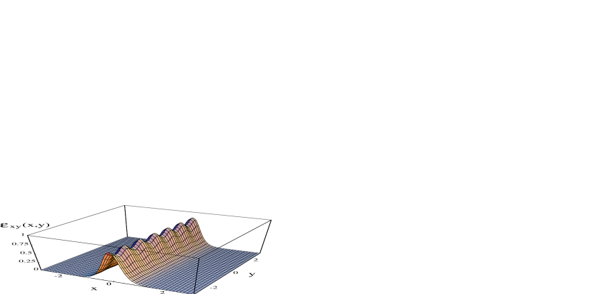
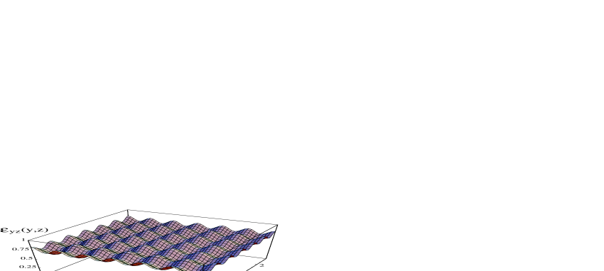
Figure 1: Action densities integrated in two directions.

B) We calculate the Wilson loop $W_{C}(r)$ around this object,

$$W_{C}(r)=\frac{1}{N}\hskip 2.84544pt{\rm Tr}\hskip 2.84544pt\left(Pexp\int_{C}\imath A_{\mu}dx_{\mu}\right)$$ (3)

being $C$ an $r\times r$ square loop in the $xt$ plane centered at the maximum of the solution. We parametrize $W_{C}(r)$ by the functions $L(r)$ (its module) and $\phi(r)$ (its phase). In figure 2 we show the quantities $L(r)$ and $\phi(r)$ as a function of $r$, putting in the same plots the values with the square loop centered at the minimum of the solutions in the $y,z$ directions and at the maximum in the $t,x$ directions. The conclusions extracted from figure 2 are the following:

• These functions are almost independent of coordinates $y$ and $z$.

• When $r$ is bigger than the size of the object we obtain $W_{C}(r)\sim exp(i4\pi/3)$, an element of the group center.

These are the two expected properties for a vortex.

Figure 2: The module $L(r)$ (top figure) and the phase $\phi(r)$ (bottom figure) of the Wilson loop defined in equation 3 as a function of $r$. Full symbols correspond to Wilson loops centered at the maximum of the solutions and empty symbols to the same quantity centered at the minimum of the solutions in the $y,z$ directions and at the maximum in the $t,x$ directions.

5 The center-projected configuration.

We apply to the obtained solutions the method of center gauge fixing. For the SU(3) vortex-like solutions we have worked with we have obtained the following maximum values: $R=0.90123970$, $0.93246431$ and $R=0.94918155$, for the lattices sizes: $N_{s}=4,5$ and $N_{s}=6$ respectively. We project the SU(N) link variables to $Z_{N}$ link variables and we calculate the values of the plaquettes from the $Z_{N}$ link variables. We obtain the following results:

• In the $xt$ plane, the plane in which the vortex is localized, we obtain for the configurations with maximum value of $R$ the same structure for all $y,z$ points. Only two plaquettes are different from the identity. The first one is located at the top-right corner and reflects the use of twisted boundary conditions. The other one is located near the maximum in the action density of the solution and has the same value of the Wilson loop shown before when the size of the loop is much bigger than the size of the solution. This is one of the most interesting results of our work, showing how the vortex properties are reflected in the center-projected configuration.

• In the $xy$ plane ( or $xz,ty,tz$ plane). In this plane the vortex is localized in one direction and almost flat in the other. There is no regular structure for all $t,z$ points. The most common configuration is that one with all plaquettes equal to the identity.

• In the $yz$ plane. The solution is almost flat in both directions. As in the previous case, there is no regular structure for all $t,x$ points. The most common configuration is that one with a very similar structure to the one in the $xt$ plane.

6 Conclusions.

The main conclusions of this work are the following two. First, our method of gauge fixing to maximal center gauge works very well. And second, we have seen that, for the configurations with maximum value of $R$, there is a clear relation between the structure of the SU(3) configuration and the structure of the center-projected one.

Acknowledgments: The present work was financed by CICYT under grant AEN97-1678. I acknowledge useful conversations with M. García Pérez, A. González-Arroyo and C. Pena.

References

- [1] L. del Debbio, M. Faber, J. Greensite and Š. Olejník, Phys. Rev. D55 (1997) 2298.
- [2] M. Faber, J. Greensite and Š. Olejník, Phys. Rev. D57 (1998) 2603.
- [3] L. del Debbio, M. Faber, J. Giedt, J. Greensite and Š. Olejník, Phys. Rev. D58 (1998) 094501.
- [4] K. Langfeld, H. Reinhardt and O. Tennert, Phys. Lett. B419 (1998) 317.
- [5] M. Engelhardt, K. Langfeld, H. Reinhardt and O. Tennert, Phys. Lett. B431 (1998) 141; Phys. Lett. B452 (1999) 301; heplat/9904004.
- [6] M. N. Chernodub, M. I. Polykarpov, A. I. Veselov and M.A. Zubkov, hep-lat/9809158.
- [7] B. L. G. Bakker, A. I. Veselov and M. A. Zubkov, hep-lat/9902010.
- [8] P. de Forcrand and M. D’Elia, Phys. Rev. Lett. 82 (1999) 4582.
- [9] P. Stephenson, Nucl. Phys. B539 (1999) 577.
- [10] A. Montero, hep-lat/9906010.
- [11] A. González-Arroyo and A. Montero, Phys. Lett. B442 (1998) 273.