July 1999

Vortex Structure vs. Monopole Dominance

in Abelian-Projected Gauge Theory

	a The Niels Bohr Institute, Blegdamsvej 17,
	DK-2100 Copenhagen Ø, Denmark.
	E-Mail: ambjorn@nbi.dk, greensit@alf.nbi.dk
	b Physics Dept., University of California at Berkeley,
	Berkeley, CA 94720 USA.
	E-mail: giedt@socrates.berkeley.edu
	c Physics and Astronomy Dept., San Francisco State Univ.,
	San Francisco, CA 94117 USA.
	E-mail greensit@stars.sfsu.edu

Abstract

We find that Polyakov lines, computed in abelian-projected SU(2) lattice gauge theory in the confined phase, have finite expectation values for lines corresponding to two units of the abelian electric charge. This means that the abelian-projected lattice has at most $Z_{2}$, rather than U(1), global symmetry. We also find a severe breakdown of the monopole dominance approximation, as well as positivity, in this charge-2 case. These results imply that the abelian-projected lattice is not adequately represented by a monopole Coulomb gas; the data is, however, consistent with a center vortex structure. Further evidence is provided, in lattice Monte Carlo simulations, for collimation of confining color-magnetic flux into vortices.

1 Introduction

The center vortex theory [1] and the monopole/abelian-projection theory [2] are two leading contenders for the title of quark confinement mechanism. Both proposals have by now accumulated a fair amount of numerical support. To decide between them, it is important to pinpoint areas where the two theories make different, testable predictions. In this article we would like to report on some preliminary efforts in that direction.

Much of the numerical work on the center vortex theory has focused on correlations between the location of center vortices, identified by the center projection method, and the values of the usual gauge-invariant Wilson loops (cf. [3], [4]). In the abelian projection approach, on the other hand, Wilson loops are generally computed on abelian projected lattices, and this fact might seem to inhibit any direct comparison of the monopole and vortex theories. However, it has also been suggested in ref. [5] that a center vortex would appear, upon abelian projection, in the form of a monopole-antimonopole chain, as indicated very schematically in Fig. 1. The idea is to consider, at fixed time, the vortex color-magnetic field in the vortex direction. In the absence of gauge fixing, the vortex field points in arbitrary directions in color space, as shown in Fig. 4. Upon fixing to maximal abelian gauge, the vortex field tends to line up, in color space, mainly in the $\pm\sigma^{3}$ direction. But there are still going to be regions along the vortex tube where the field rotates from the $+\sigma_{3}$ to the $-\sigma_{3}$ direction in color space (Fig. 4). Upon abelian projection, these regions show up as monopoles or antimonopoles, as illustrated in Fig. 4. If this picture is right, then the $\pm 2\pi$ monopole flux is not distributed symmetrically on the abelian-projected lattice, as one might expect in a Coulomb gas. Rather, it will be collimated in units of $\pm\pi$ along the vortex line. We have argued elsewhere [6] that some sort of collimation of monopole magnetic fields into units of $\pm\pi$ is likely to occur even in the $D=3$ Georgi-Glashow model, albeit on a scale which increases exponentially with the mass of the W-boson. On these large scales, the ground state of the Georgi-Glashow model cannot be adequately represented by the monopole Coulomb gas analyzed by Polyakov in ref. [7]. The question we address here is whether such flux collimation also occurs on the abelian-projected lattice of $D=4$ pure Yang-Mills theory.

Figure 1: Hypothetical collimation of monopole/antimonopole flux into center vortex tubes on the abelian-projected lattice.

The test of flux collimation on abelian-projected lattices is in principle quite simple. Consider a very large abelian Wilson loop

$$W_{q}(C)=\Big{<}\exp[iq\oint dx^{\mu}A_{\mu}]\Big{>}$$ (1.1)

or abelian Polyakov line

$$P_{q}=\Big{<}\exp[iq\int dtA_{0}]\Big{>}$$ (1.2)

corresponding to $q$ units of the electric charge. The expectation values are obtained on abelian-projected lattices, extracted in maximal abelian gauge. If $q$ is an even number, then magnetic flux of magnitude $\pm\pi$ through the Wilson loop will not affect the loop. Flux collimation therefore implies that $W_{q}(C)$ has an asymptotic perimeter-law falloff if $q$ is even. Likewise, Polyakov lines $P_{q}$ for even $q$ are not affected, at long range, by collimated vortices of $\pm\pi$ magnetic flux. In the confined phase, the prediction is that $P_{q}=0$ only for odd-integer $q$. In contrast, we expect in a monopole Coulomb gas of the sort analyzed by Polyakov that $W_{q}(C)$ has an area-law falloff, and $P_{q}=0$, for all $q$.

Figure 2: Vortex field strength before gauge fixing. The arrows indicate direction in color space.

Figure 3: Vortex field strength after maximal abelian gauge fixing. Vortex field strength is mainly in the $\pm\sigma_{3}$ direction

Figure 4: Vortex field after abelian projection.

Numerical results for abelian-projected Wilson loops and Polyakov lines must be interpreted with some caution in the usual maximal abelian gauge, due to the absence of a transfer matrix in this gauge. Since positivity is not guaranteed, these expectation values need not relate directly to the energies of physical states. For this reason, we prefer to interpet the abelian observables in terms of the type of global symmetry, or type of “magnetic disorder”, present in the abelian-projected lattice, without making any direct reference to the potential between abelian charges, or the energies of isolated charges. Following ref. [6], let us introduce the U(1) holonomy probability distribution on abelian-projected lattices

$${\cal P}_{C}[g]=\Big{<}\delta\left[g,\exp(i\oint dx^{\mu}A_{\mu})\right]\Big{>}$$ (1.3)

for Wilson loops, and

$${\cal P}_{T}[g]=\Big{<}\delta\left[g,\exp(i\int dtA_{0})\right]\Big{>}$$ (1.4)

for Polyakov lines, where

$$\delta\Bigl{[}e^{i\theta_{1}},e^{i\theta_{2}}\Bigr{]}={1\over 2\pi}\sum_{n=-\infty}^{\infty}e^{in(\theta_{2}-\theta_{1})}$$ (1.5)

is the $\delta$-function on the U(1) manifold. These distributions give us the probability density that a given abelian Wilson loop around curve $C$, or an abelian Polyakov line of length $T$, respectively, will be found to have the value $g\in U(1)$ in any thermalized, abelian-projected lattice. The lattice has global U(1) symmetry (or, in alternative terminology, the lattice has “U(1) magnetic disorder”) if these distributions are flat for Polyakov lines and large Wilson loops. In other words, we have U(1) symmetry iff, for any $g,g^{\prime}\in U(1)$, it is true that

$${\cal P}_{T}[g]-{\cal P}_{T}[g^{\prime}g]=0$$ (1.6)

for Polyakov lines, and

$${\cal P}_{C}[g]-{\cal P}_{C}[g^{\prime}g]\sim\exp[-\sigma\mbox{Area}(C)]$$ (1.7)

holds asymptotically for large Wilson loops. In the case that these relations are not true in general, but the restricted forms

$${\cal P}_{T}[g]-{\cal P}_{T}[zg]=0$$ (1.8)

and

$${\cal P}_{C}[g]-{\cal P}_{C}[zg]\sim\exp[-\sigma\mbox{Area}(C)]$$ (1.9)

hold for any $g\in U(1)$ and $z=\pm 1\in Z_{2}$, then we will say that the lattice has only $Z_{2}$ global symmetry (or $Z_{2}$ magnetic disorder).

Inserting (1.5) into (1.3) and (1.4), we have

$${\cal P}_{C}[e^{i\theta}] = {1\over 2\pi}\left(1+2\sum_{q>0}W_{q}(C)\cos(q\theta)\right)$$

$${\cal P}_{T}[e^{i\theta}] = {1\over 2\pi}\left(1+2\sum_{q>0}P_{q}\cos(q\theta)\right)$$ (1.10)

From this, we can immediately see that there is U(1) magnetic disorder iff $W_{q}(C)$ has an asymptotic area law falloff, and $P_{q}=0$, for all integer $q\neq 0$. On the other hand, if these conditions hold only for $q=$odd integer, then we have $Z_{2}$ magnetic disorder. It is an unambiguous prediction of the vortex theory that the lattice has only $Z_{2}$ magnetic disorder, even after abelian projection.

The magnetic disorder induced by a monopole Coulomb gas is expected to be rather different from the disorder induced by vortices. A Coulombic magnetic field distribution will in general affect loops of any $q$, with $q>1$ loops responding even more strongly than $q=1$ to any variation of magnetic flux through the loop. The usual statement is that all integer abelian charges are confined. This statement is confirmed explicitly in $D=3$ dimensions, where it is found in a semiclassical calculation that the monopole Coulomb gas derived from $QED_{3}$ confines all charges, with string tensions $\sigma_{q}$ directly proportional to the charge [6]

$$\sigma_{q}=q\sigma_{1}$$ (1.11)

This relation is also consistent with recent numerical simulations [8].

In D=4 dimensions, an analytic treatment of monopole currents interacting via a two-point long-range Coulomb propagator, plus possible contact terms, is rather difficult. Nevertheless, $QED_{4}$ (particularly in the Villain formulation) can be viewed as a theory of monopole loops and photons, and in the confined (=strong-coupling) phase there is a string tension for all charges $q$, and all $P_{q}=0$, as can be readily verified from the strong-coupling expansion. Confinement of all charges $q$ is also found in a simple model of the monopole Coulomb gas, due to Hart and Teper [9]. Finally, all multiples $q$ of electric charge are confined in the dual abelian Higgs model (a theory of dual superconductivity), and this model is known [10] to be equivalent, in certain limits, to an effective monopole action with long-range two-point Coulombic interactions between monopole currents.

In the case of $D=4$ abelian-projected Yang-Mills theory, we do not really know if the distribution of monopole loops identified on the projected lattice is typical of a monopole Coulomb gas. What can be tested, however, is whether or not the field associated with these monopoles is Coulombic (as opposed, e.g., to collimated). This is done by comparing observables measured on abelian-projected lattices with those obtained numerically via a “monopole dominance” (MD) approximation, first introduced in ref. [12]. The MD approximation involves two steps. First, the location of monopole currents on an abelian-projected lattice is identified using the standard DeGrand-Toussaint criterion [13]. Secondly, a lattice configuration is reconstructed by assuming that each link is affected by the monopole currents via a lattice Coulomb propagator. Thus, the lattice Monte Carlo and abelian projection supply a certain distribution of monopoles, and we can study the consequences of assigning a Coulombic field distribution to the monopole charges.

We should pause here, to explain how the non-confinement of color charges in the adjoint representation is accounted for in the monopole gas or dual-superconductor pictures, in which all abelian charges are confined. The screening of adjoint (or, in general, $j=$integer) representations in Yang-Mills theory is a consequence of having only $Z_{2}$ global symmetry on a finite lattice in the confined phase. In a monopole Coulomb gas, on the other hand, the confinement of all abelian charges would imply a U(1) global symmetry of the projected lattice at finite temperature. Nevertheless, the $Z_{2}$ symmetry of the full lattice and U(1) symmetry of the projected lattice are not necessarily inconsistent. Let $P^{YM}_{j}$ represent the Polyakov line in SU(2) gauge theory in group representation $j$. Generalizing eq. (1.4) to $g\in SU(2)$, we have

$${\cal P}_{T}[g]=\sum_{j=0,\frac{1}{2},1...}P^{YM}_{j}\chi_{j}[g]$$ (1.12)

and the fact that eq. (1.8), rather than eq. (1.6), is satisfied follows from the identity

$$\chi_{j}(zg)=\chi_{j}(g)~{}~{}~{}~{}\mbox{for~{}}j=\mbox{integer}$$ (1.13)

and from the fact that

$$P^{YM}_{j}\left\{\begin{array}[]{rl}=0&j=\mbox{half-integer}\cr\neq 0&j=\mbox{integer}>0\end{array}\right.$$ (1.14)

in the confined phase, due to confinement of charges in half-integer, and color-screening of charges in integer, SU(2) representations.

Now, on an abelian projected lattice, the expectation value of a Yang-Mills Polyakov line in representation $j$ becomes

$$P^{YM}_{j}\rightarrow\sum_{m=-j}^{j}P_{2m}$$ (1.15)

where $P_{q}$ is the abelian Polyakov line defined in eq. (1.2). If the abelian-projected lattice is U(1) symmetric, then $P_{2m}=0$ for all $m\neq 0$, while $P_{0}=1$. This means that after abelian-projection we have

$$P^{YM}_{j}=\left\{\begin{array}[]{rl}0&j=\mbox{half-integer}\cr 1&j=\mbox{integer}\end{array}\right.$$ (1.16)

and in this way the non-zero values of $j=$integer Polyakov lines are accounted for, even assuming that the projected lattice has a global U(1)-invariance. Similarly, adjoint Wilson loops will not have an area law falloff on the projected lattice, as expected from color-screening. This explanation of the adjoint perimeter law in the abelian projection theory has other difficulties, associated with Casimir scaling of the string tension at intermediate distances (cf. ref. [11]), but at least the asympotic behavior of Wilson loops in various representations is consistent with U(1) symmetry on the abelian projected lattice.

It is just this assumed U(1) symmetry of the abelian-projected lattice, and the monopole Coulomb gas picture which is associated with it, that we question here. The U(1) vs. $Z_{2}$ global symmetry issue can be settled by calculating abelian Wilson loops and/or Polyakov lines for abelian charges $q>1$. The validity of the Coulomb gas picture can also be probed by calculating $W_{q}(C)$ and $P_{q}$ with and without the monopole dominance (MD) approximation, and comparing the two sets of quantities.

The first calculation of $q>1$ Wilson loops, in the MD approximation, was reported recently by Hart and Teper [9]; their calculation confirms the Coulomb gas relation $\sigma_{q}\propto q$ found previously for compact $QED_{3}$. In ref. [9], this result is interpreted as favoring the monopole Coulomb gas picture over the vortex theory. From our previous remarks, it may already be clear why we do not accept this interpretation. At issue is whether monopole magnetic fields spread out as implied by the Coulomb propagator, or whether they are collimated in units of $\pm\pi$. This issue cannot be resolved by the MD approximation, which imposes a Coulombic field distribution from the beginning. The MD approximation does, however, tell us that if the monopoles have a Coulombic field distribution, then the $q=2$ Wilson loop has an area law falloff, at least up to the maximum charge separation studied in ref. [9]. The crucial question is whether the $q=2$ loops computed directly on abelian projected lattices also have an asymptotic area law falloff, or instead go over to perimeter-law behavior (usually called “string-breaking”) as predicted by the vortex theory.

Here it is important to have some rough idea of where the $q=2$ string is expected to break, according to the vortex picture, otherwise a null result can never be decisive. A $q=2$ Wilson loop will go over to perimeter behavior when the size of the loop is comparable to the thickness of the vortex. It seems reasonable to assume that the thickness of a vortex on the abelian-projected lattice is comparable to the thickness of a center vortex on the unprojected lattice. From Fig. 1 of ref. [3], this thickness appears to be roughly one fermi, which is also about the distance where an adjoint representation string should break in $D=4$, according to an estimate due to Michael [16]. The finite thickness of the vortex is an important feature of the vortex theory, as it allows us to account for the approximate Casimir scaling of string tensions at intermediate distances (cf. refs. [17, 18]). But it also means that at, e.g., $\beta=2.5$, we should look for string breaking at around $R=12$ lattice spacings. Noise reduction techniques, such as the “thick-link” approach, then become essential.

The validity of the thick-link approach, however, is tied to the existence of a transfer matrix. Since the method uses $R\times T$ loops with $R\gg T$, one has to show that the potential extracted is mainly sensitive to the large separation $R$, rather than the smaller separation $T$, and here positivity plays a crucial rule. Since there is no transfer matrix in maximal abelian gauge, the validity of the thick link approach is questionable (and the issue of positivity is much more than a quibble, as we will see below). Moreover, even when a transfer matrix exists, string-breaking is not easy to observe by this method, and requires more than just the calculation of rectangular loops. The breaking of the adjoint-representation string has not been seen using rectangular loops alone, and only quite recently has this breaking been observed, in 2+1 dimensions, by taking account of mixings between string and gluelump operators [14, 15]. The analogous calculation, for operators defined in maximal abelian gauge, would presumably involve mixings between the $q=2$ string and “charge-lumps”; the latter being bound states of the static abelian charge and the off-diagonal (double abelian-charged) gluons.

There are, in fact, existing calculations of the $q=2$ potential, by Poulis [19] and by Bali et al. [20], using the thick-link method. String breaking was not observed, but neither did these calculations make use of operator-mixing techniques, which seem to be necessary for this purpose. In any case, in view of the absence of a transfer matrix in maximal abelian gauge, we do not regard these calculations as decisive.

Given our reservations concerning the thick-link approach, we will opt in this article for a far simpler probe of global symmetry/magnetic disorder on the projected lattice, namely, the double-charged abelian Polyakov lines $P_{2}$. Any abelian magnetic vortex can be regarded, away from the region of non-vanishing vortex field strength, as a discontinuous gauge transformation, and it is this discontinuity which affects Wilson loops and Polyakov lines far from the region of finite vortex field strength. If the vortex flux is $\pm\pi$, the discontinuity will not affect even-integer $q$-charged Polyakov lines, and these should have a finite expectation value. The abelian-projected lattice then has only $Z_{2}$ global symmetry in the confined phase. In contrast, a monopole Coulomb gas is expected to confine all $q$ charges, as in compact $QED_{3}$, and the $Z_{2}$ subgroup should play no special role. In that case, $P_{q}=0$ for all $q$. Thus, if we find that the $q=2$ Polyakov line vanishes, this is evidence against vortex structure and flux collimation, and in favor of the monopole picture. Conversely, if $q=2$ Polyakov lines do not vanish, the opposite conclusion applies, and the vortex theory is favored.

2 Polyakov lines

After fixing to maximal abelian gauge in SU(2) lattice gauge theory, abelian link variables

$$U^{A}_{\mu}(x)=\mbox{diag}[e^{i\theta_{\mu}(x)},e^{-i\theta_{\mu}(x)}]$$ (2.1)

are extracted by setting the off-diagonal elements of link variables $U_{\mu}$ to zero, and rescaling to restore unitarity. A $q$-charge Polyakov line $P_{q}(\vec{x})$ is defined as

$$P_{q}(\vec{x})=\prod_{n=1}^{N_{T}}\exp[iq\theta_{4}(\vec{x}+n\hat{4})]$$ (2.2)

where $N_{T}$ ($N_{S}$) is the number of lattice spacings in the time (space) directions. We can consider both the expectation value of the lattice average

$$P_{q}=\left<{1\over N_{S}^{3}}\sum_{\vec{x}}P_{q}(\vec{x})\right>$$ (2.3)

and the expectation value of the absolute value of the lattice average

$$P^{abs}_{q}=\left<{1\over N_{S}^{3}}\left|\sum_{\vec{x}}P_{q}(\vec{x})\right|\right>$$ (2.4)

Polyakov lines can vanish for $q=1$, even in the deconfined phase, just by averaging over $Z_{2}$-degenerate vacua, which motivates the absolute value prescription. In the confined phase, one then has $P^{abs}_{1}\sim N_{S}^{-3/2}$. We will find that this prescription is unnecessary for $q=2$, and we will compute these Polyakov lines without taking the absolute value of the lattice average.

For purposes of comparison, and as a probe of the monopole Coulomb gas picture, we also compute “monopole” Polyakov lines $P_{Mq}$ following an MD approach used by Suzuki et al. in ref. [21]. Their procedure is to decompose the abelian plaquette variable ($\partial_{\mu}$ denotes the forward lattice difference)

$$f_{\mu\nu}(x)=\partial_{\mu}\theta_{\nu}(x)-\partial_{\nu}\theta_{\mu}(x)$$ (2.5)

into two terms

$$f_{\mu\nu}(x)=\overline{f}_{\mu\nu}(x)+2\pi n_{\mu\nu}(x)$$ (2.6)

where $n_{\mu\nu}$ is an integer-valued Dirac-string variable, and $-\pi<\overline{f}_{\mu\nu}\leq\pi$. One can then invert (2.5) to solve for $\theta_{4}$ in terms of the “photon” field-strength $\overline{f}_{\mu\nu}$, the Dirac-string variables $n_{\mu\nu}$, and an irrelevant U(1) gauge-dependent term. If we assume that the photon and Dirac-string variables are completely uncorrelated, then the Dirac-string contribution is given by

$$\theta^{M}_{4}(x)=-\sum_{x^{\prime}}D(x,x^{\prime})\partial^{\prime}_{\nu}n_{\nu 4}(x^{\prime})$$ (2.7)

Here $D(x,x^{\prime})$ is the lattice Coulomb propagator, and the partial derivative denotes a backward difference. The monopole dominance approximation is to replace $\theta_{4}$ by $\theta^{M}_{4}$ in eq. (2.2), the idea being that this procedure isolates the contribution of the monopole fields to the Polyakov lines. The correlations between the photon, monopole, and abelian lattice fields will be discussed in more detail in section 3, and in an Appendix.

2.1 $Z_{2}$ Magnetic Disorder

In Fig. 5 we display $P^{abs}_{1}$ and $P^{abs}_{M1}$ for the $q=1$ lines, on a $12^{3}\times 3$ lattice. There are no surprises here; we see that for $N_{T}=3$ there is a deconfinement transition around $\beta=2.15$.

Figure 5: Single charge ($q=1$) Polyakov lines at time extention T=3, on the abelian projected lattice and in the monopole dominance (MD) approximation.

The situation changes dramatically when we consider $q=2$ Polyakov lines. Fig. 6 is a plot of the values of $P_{2}$ and $P_{M2}$, without any absolute value prescription, on the $12^{3}\times 3$ lattice. To make the point clear, we focus on the data in the confined phase, in Fig. 7. It can be seen that $P_{2}$ is non-vanishing and negative in the confined phase; the data is clearly not consistent with a vanishing expectation value. In the MD approximation, $P_{M2}$ may also be slightly negative, but its value is at least an order of magnitude smaller than $P_{2}$. This seems to be a very strong breakdown of monopole dominance, in the form proposed in ref. [21].

Figure 6: Doubly-charged ($q=2$) Polyakov lines at time extension T=3, on the abelian projected lattice and in the monopole dominance (MD) approximation.

Figure 7: Magnified view of $q=2$ abelian and monopole-dominance Polyakov lines at time extension $T=3$, in the confined phase.

In Figures 8-10 we plot the corresponding data found on a $16^{3}\times 4$ lattice. There is a deconfinement transition close to $\beta=2.3$, and again there is a clear disagreement between $P_{2}$ and $P_{M2}$, with the former having a substantial non-vanishing expectation value throughout the confined phase.

Figure 8: $q=1$ Polyakov lines (as in Fig. 5), for time extension T=4 lattice spacings.

Figure 9: $q=2$ Polyakov lines (as in Fig. 6), for time extension T=4 lattice spacings.

Figure 10: $q=2$ Polyakov lines in the confined phase (as in Fig. 7), for time extension T=4 lattice spacings.

The numerical evidence, for both $T=3$ and $T=4$, clearly favors having $Z_{2}$, rather than U(1), global symmetry/magnetic disorder on the abelian projected lattice.

2.2 Spacelike Maximal Abelian Gauge

It is also significant that $P_{2}$ is negative. This implies a lack of reflection positivity in the Lagrangian obtained after maximal abelian gauge fixing, and must be tied to the fact that maximal abelian gauge is not a physical gauge. This diagnosis also suggests a possible cure: Instead of fixing to the standard maximal abelian gauge, which maximizes

$$R=\sum_{x}\sum_{\mu=1}^{4}\mbox{Tr}[\sigma_{3}U_{\mu}(x)\sigma_{3}U^{\dagger}_{\mu}(x)]$$ (2.8)

we could try to use a “spacelike” maximal abelian gauge [22], maximizing the quantity

$$R=\sum_{x}\sum_{k=1}^{3}\mbox{Tr}[\sigma_{3}U_{k}(x)\sigma_{3}U^{\dagger}_{k}(x)]$$ (2.9)

which involves only links in spatial directions. This is a physical gauge. What happens in this case is that one disease, the loss of reflection positivity, it replaced by another, namely, the breaking of $90^{\circ}$ rotation symmetry. This is illustrated in Fig. 11, where we plot spacelike and timelike Polyakov lines on a $4^{4}$ lattice, in the spacelike maximal abelian gauge defined above. We find that the values for double-charged Polyakov lines running in the time direction are much reduced in the spacelike gauge, and in fact the results shown appear consistent with zero. Spacelike $q=2$ Polyakov lines, however, which run along the $1,2,$ or $3$ lattice directions, remain negative, and in fact are larger in magnitude than Polyakov lines of the same length, and the same coupling, computed in the usual maximal abelian gauge. One therefore finds on a hypercubic lattice that $90^{\circ}$ rotation symmetry is broken.

The spacelike Polyakov line operator creates a line of electric flux through the periodic lattice. The non-vanishing overlap of this state with the vacuum has, in the spacelike gauge, a direct physical interpretation: Since the $q=2$ electric flux line cannot, for topological reasons, shrink to zero, a finite overlap with the vacuum means that the $q=2$ flux tube breaks. This is presumably due to screening by double-charged (off-diagonal) gluon fields. The implication is that in a physical gauge, where Wilson loops can be translated into statements about potential energies, $q=$ even abelian charges are not confined.

Figure 11: Breaking of $90^{\circ}$ rotation symmetry in spacelike maximal abelian gauge, as seen from comparing timelike Polyakov lines (lattice 4 direction) with spacelike Polyakov lines (lattice 1,2, or 3 directions) on a $4^{4}$ lattice.

The fact that $q=$ even charges are unconfined, together with the positivity property in spacelike maximal abelian gauge, leads to the conclusion that timelike $q=2$ Polyakov lines $P_{2}$ are positive and non-zero, although the data points for timelike $P_{2}$ shown in Fig. 11, which appear to be consistent with zero, do not yet support such a conclusion. It must be that the value of $P_{2}$ in this gauge is simply very small, and much better statistics are required to distinguish that value from zero. To get some idea of the difficulty involved, let us suppose that the magnitude of the timelike abelian line $P_{2}$ on the projected lattice is comparable to the magnitude of the gauge-invariant Polyakov line $P_{adj}$, in the adjoint representation of SU(2), on the full, unprojected lattice. To leading order in the strong-coupling expansion, $P_{adj}$ on a lattice with extension $T$ in the time direction is given by

$$P_{adj}=4\left({\beta\over 4}\right)^{4T}$$ (2.10)

This equals, e.g., $0.00156$ for $T=2$ at $\beta=1.5$; quite a small signal considering that $T$ is only two lattice units. The obvious remedy is to increase $\beta$, but then one runs into a deconfinement transition at $\beta=1.8$. We can move the transition to larger $\beta$ by increasing $T$, but of course increasing $T$ again causes the signal to go down.

The best chance to extract a signal from the noise is to choose a value of $\beta$ which is fairly close to the deconfinement transition (but still in the confined phase), and to generate very many configurations. Here are the results obtained at $T=2$ lattice spacings and $\beta=1.7$, coming from 5000 configurations separated by 100 sweeps on a $2\times 8^{3}$ lattice:

$$P_{adj} = 0.00447(23)$$

$$P_{2} = 0.00241(52)$$ (2.11)

The result for the adjoint line is consistent with the strong-coupling prediction of $P_{adj}=0.00426$. The abelian line $P_{2}$ is non-zero, positive, and comparable in magnitude to $P_{adj}$, although it must be admitted that the errorbar is uncomfortably large. The corresponding values for $T=3$ and $\beta=2.11$, obtained from 5000 $3\times 8^{3}$ lattices, are

$$P_{adj} = 0.00338(28)$$

$$P_{2} = 0.00124(42)$$ (2.12)

Again $P_{2}$ is non-zero, although the errorbar is still too large for comfort.

Clearly the evaluation of the timelike $P_{2}$ line in spacelike maximal abelian gauge is cpu-intensive, and our results for this quantity must be regarded as preliminary. Nevertheless, these preliminary results are consistent with the conclusion previously inferred from the spacelike lines: In a physical gauge, the $q=2$ charge is screened, rather than confined, and we have $Z_{2}$, rather than U(1), magnetic disorder on the abelian-projected lattice.

3 The “Photon” Contribution

Suppose we write the link angles $\theta_{\mu}(x)$ of the abelian link variables as a sum of the link angles $\theta^{M}_{\mu}(x)$ in the MD approximation, plus a so-called “photon” contribution $\theta^{ph}_{\mu}(x)$, i.e.

$$\theta^{ph}_{\mu}(x)\equiv\theta_{\mu}(x)-\theta_{\mu}^{M}(x)$$ (3.1)

It was found in refs. [12, 21, 23] that the photon field has no confinement properties at all; the Polyakov line constructed from links $U_{\mu}=\exp[i\theta^{ph}_{\mu}]$ is finite, and corresponding Wilson loops have no string tension. Since $\theta_{\mu}^{M}$ would appear to carry all the confining properties, a natural conclusion is that the abelian lattice is indeed a monopole Coulomb gas.

To see where this reasoning may go astray, suppose we perversely add, rather than subtract, the MD angles to the abelian angles, i.e.

$$\theta^{\prime}_{\mu}(x) = \theta_{\mu}(x)+\theta_{\mu}^{M}(x)$$ (3.2)

$$= \theta^{ph}_{\mu}(x)+2\theta_{\mu}^{M}(x)$$

in effect doubling the strength of the monopole Coulomb field. It is natural to expect a corresponding increase of the string tension, and of course $P_{1}=0$ should remain true. Surprisingly, this is not what happens; doubling the strength of the monopole field in fact removes confinement. Some results for $P_{1}$ are shown in Table 1. Here we have computed the vev of $P_{1}(x)$ without taking the absolute value of the lattice sum (i.e. we use eq. (2.3) rather than eq. (2.4)), and we find that $P_{1}$ is finite and negative in the additive configurations. The additive configuration $\theta^{\prime}$ is far from pure-gauge, and the vev of $P_{1}$ is correspondingly small. Nevertheless, $P_{1}$ is non-zero, so adding the monopole field in this case actually removes confinement. Clearly, the interplay between the MD and “photon” contributions is a little more subtle than previously supposed.

T $\beta$ $P_{1}$ line 3 1.8 -0.0299 (20) 3 2.1 -0.0405 (10) 4 2.1 -0.0134 (10)

Table 1: Single-charged abelian Polyakov lines, computed in the additive $\theta^{\prime}=\theta+\theta^{M}$ configurations, in which the strength of the MD contribution is effectively doubled.

To understand what is going on, we return to the concept of the holonomy probability distribution

$${\cal P}(\theta)={\cal P}_{T}[e^{i\theta}]=\Big{<}\delta\left[e^{i\theta},\prod_{n=1}^{N_{T}}\exp[i\theta_{4}(\vec{x}+n\hat{4})]\right]\Big{>}$$ (3.3)

${\cal P}_{T}[e^{i\theta}]$ is the probability density for the U(1) group elements on the group manifold. However, since the group measure on the U(1) manifold is trivial (i.e. $d\theta$), it is not hard to see that ${\cal P}(\theta)d\theta$ is interpreted as the probability that the phase of an abelian Polyakov line lies in the interval $[\theta,\theta+d\theta]$. In a similar way, replacing $\theta_{4}$ by $\theta^{M}_{4}$ or $\theta^{ph}_{4}$ on the rhs of the above equation, we can define the probability distributions ${\cal P}(\theta^{M})$ and ${\cal P}(\theta^{ph})$, respectively, for the phases of monopole and photon Polyakov lines. All of these distributions have $2\pi$-periodicity, and are invariant under $\theta\rightarrow-\theta$, reflections, so we need only consider their behavior in the interval $[0,\pi]$. Without making any further calculations, it is already possible to deduce something about the shape of ${\cal P}(\theta)$:

• Since all $P_{q}$ are small, ${\cal P}(\theta)$ is fairly flat.

• Assuming $Z_{2}$ symmetry, ${\cal P}(\theta)$ is symmetric, in the interval $[0,\pi]$, around $\theta={\pi\over 2}$.

• Since $P_{2}$ is negative, ${\cal P}(\theta)$ should be larger in the neighborhood of $\theta={\pi\over 2}$ than in the neighborhood of $\theta=0$ or $\theta=\pi$.

From these considerations, we deduce that ${\cal P}(\theta)$ looks something like Fig. 12. Similarly, since $P_{Mq}\approx 0$ in the MD approximation, we conclude that there is very nearly U(1) symmetry in this approximation, and ${\cal P}(\theta^{M})$ is almost flat, as in Fig. 13.

Figure 12: Conjectured ${\cal P}(\theta)$ distribution of the Polyakov phase angle, based on $Z_{2}$ global symmetry and $P_{2}<0$.

Figure 13: ${\cal P}(\theta^{M})$ in the MD approximation, assuming perfect global U(1) symmetry.

Figure 14: The “photon” angle distribution ${\cal P}(\theta^{ph})$, resulting from a correlation between $\theta$ and $\theta^{M}$.

Now if the link angles $\theta_{\mu}(x)$ and $\theta^{M}_{\mu}(x)$ are correlated to some extent, then the difference $\theta^{ph}(x)$ between these variables is not random, but has some non-uniform probability distribution as illustrated in Fig. 14. Since the Fourier cosine components of ${\cal P}(\theta^{ph})$ are typically non-zero, it follows that the photon field, by itself, has no confinement property. The crucial point is that by subtracting $\theta^{M}$, the $Z_{2}$ symmetry of $\theta$ is broken due to the correlation between $\theta$ and $\theta^{M}$. It is interesting to note that even if ${\cal P}(\theta^{M})$ were neither U(1) nor $Z_{2}$ symmetric, i.e. if we imagine that the $\theta$-configurations confine but the MD contributions do not, a correlation between the $\theta$ and $\theta^{M}$ would still be sufficient to break the $Z_{2}$ symmetry of the difference configuration $\theta^{ph}$. As a result, subtracting the non-confining $\theta^{M}$ from the confining $\theta$ would still remove confinement.

In the center vortex picture, vortex fields supply the confining disorder, but of course this does not at all exclude a correlation of the MD variables $\theta^{M}$ with the $\theta$ variables. According to the arguments in the Introduction, monopoles lie along vortices as shown in Fig. 1 (further evidence is given in the next section), and this correspondence will certainly introduce some degree of correlation between magnetic flux on the abelian-projected lattice, and magnetic flux in the MD approximation. Roughly speaking, one can say that the confining flux has the same magnitude on the abelian and MD lattices, only it is distributed differently (collimated vs. Coulombic). However, according to the center vortex picture, there must also be some correlation between $\theta^{ph}_{\mu}(x)$ and $\theta^{M}_{\mu}(x)$; this is necessary to convert the long-range monopole Coulomb field into a vortex field, and to break the U(1) symmetry of the MD lattice down to the $Z_{2}$ symmetry of the vortex vacuum.

In numerical simulations performed at $\beta=2.1$ and $T=3$ on a $3\times 12^{3}$ lattice, we do, in fact, find a striking correlation between $\theta^{ph}$ and $\theta^{M}$: The average “photon” angle $\theta^{ph}$ tends to be positive for $\theta^{M}\in[0,{\pi\over 2}]$, and negative for $\theta^{M}\in[{\pi\over 2},\pi]$. Computing the average photon angle $\overline{\theta}^{ph}$ in each monopole angle quarter-interval, we find

$$\overline{\theta}^{ph}=\left\{\begin{array}[]{rl}0.027(4)&\mbox{for~{}~{}}\theta^{M}\in[0,{\pi\over 2}]\cr-0.027(4)&\mbox{for~{}~{}}\theta^{M}\in[{\pi\over 2},\pi]\end{array}\right.$$ (3.4)

This result, combined with the results displayed in Table 1, raises two interesting questions:

1. How is the correlation between $\theta^{ph}$ and $\theta^{M}$, found above in (3.4), related to the remaining $Z_{2}$ global symmetry of ${\cal P}(\theta)$; and

2. Why is $P_{1}$ negative in the additive configurations of eq. (3.2)?

To shed some light on these issues, we begin by defining $\overline{\theta}^{ph}(\theta^{M})$ as the average value of $\theta^{ph}$ at fixed $\theta^{M}$, and then make the drastic approximation of neglecting all fluctuations of $\theta^{ph}$ at fixed $\theta^{M}$ around its mean value. This amounts to approximating the vev of any periodic function $F(\theta)$

$$<F>=\int^{\pi}_{-\pi}d\theta~{}F(\theta){\cal P}(\theta)$$ (3.5)

by

$$<F>=\int^{\pi}_{-\pi}d\theta^{M}{1\over 2\pi}F(\theta^{M}+\overline{\theta}^{ph}(\theta^{M}))$$ (3.6)

where we have used the fact that the probability distribution for $\theta^{M}$ is (nearly) uniform. The accuracy of this approximation depends, of course, on the width of the probability distribution for $\theta^{ph}$ at fixed $\theta^{M}$, and on the particular $F(\theta)$ considered. Here we are only concerned with certain qualitative aspects of phase angle probability distributions, and hopefully the neglect of fluctuations of $\theta^{ph}$ around the mean will not severely mislead us.

With the help of the approximation (3.6), we can answer the two questions posed above. In this section we will only outline the argument, which is presented in full in an Appendix.

The function $\overline{\theta}^{ph}(\theta^{M})$ maps the variable $\theta^{M}\in[-\pi,\pi]$, which has a uniform probability distribution in the interval, into the variable $\overline{\theta}\in[-\pi,\pi]$, where

$$\overline{\theta}=\theta^{M}+\overline{\theta}^{ph}(\theta^{M})$$ (3.7)

The non-uniform mapping induces a non-uniform probability distribution for the $\overline{\theta}$-variable

$${\cal P}(\overline{\theta}) = {1\over 2\pi}{d\theta^{M}\over d\overline{\theta}}$$ (3.8)

$$= {1\over 2\pi}\left(1-{d\overline{\theta}^{ph}\over d\overline{\theta}}\right)$$

which we identify with ${\cal P}(\theta)$ in the approximation (3.6). Since ${\cal P}(\theta)$ is peaked at $\theta=\pm{\pi\over 2}$, it follows that $d\overline{\theta}^{ph}/d\overline{\theta}$ is minimized at $\overline{\theta}=\pm{\pi\over 2}$.

Global $Z_{2}$ symmetry implies that $P_{q}=0$ for $q=$ odd. Then, from eq. (1.10) we have

$${\cal P}(\pi-\overline{\theta}) = {\cal P}(\overline{\theta})$$

$${\cal P}(-\pi-\overline{\theta}) = {\cal P}(\overline{\theta})$$

$${\cal P}(-\overline{\theta}) = {\cal P}(\overline{\theta})$$ (3.9)

From these relationships, eq. (3.8), and the fact (shown in the Appendix) that $\overline{\theta}^{ph}(-\theta^{M})=-\overline{\theta}^{ph}(\theta^{M})$, we find that

$$\overline{\theta}^{ph}[\overline{\theta}]\equiv\overline{\theta}^{ph}[\theta^{M}(\overline{\theta})]$$ (3.10)

is an odd function with respect to reflections around $\overline{\theta}=0,\pm{\pi\over 2}$. Defining $\overline{\theta}^{ph}_{I}$ as the average $\theta^{ph}$ in the quarter interval $\theta^{M}\in[0,{\pi\over 2}]$, and $\overline{\theta}^{ph}_{II}$ as the average $\theta^{ph}$ in the quarter-interval $\theta^{M}\in[{\pi\over 2},\pi]$, we have

$$\overline{\theta}^{ph}_{I} = {2\over\pi}\int_{0}^{\pi/2}d\theta^{M}~{}\overline{\theta}^{ph}(\theta^{M})$$ (3.11)

$$= 4\int_{0}^{\pi/2}d\overline{\theta}~{}{\cal P}(\overline{\theta})\overline{\theta}^{ph}[\overline{\theta}]$$

$$= 4\int_{\pi/2}^{\pi}d\overline{\theta}~{}{\cal P}(\pi-\overline{\theta})\overline{\theta}^{ph}[\pi-\overline{\theta}]$$

$$= -4\int_{\pi/2}^{\pi}d\overline{\theta}~{}{\cal P}(\overline{\theta})\overline{\theta}^{ph}[\overline{\theta}]$$

$$= -{2\over\pi}\int_{\pi/2}^{\pi}d\theta^{M}~{}\overline{\theta}^{ph}(\theta^{M})$$

$$= -\overline{\theta}^{ph}_{II}$$

which explains, as a consequence of global $Z_{2}$ symmetry, the equal magnitudes and opposite signs found in eq. (3.4). This answers the first of the two questions posed above.

For expectation values of Polyakov phase angles in the additive configuration, we have

$$<F>=\int^{\pi}_{-\pi}d\theta^{\prime}~{}F(\theta^{\prime}){\cal P}^{\prime}(\theta^{\prime})$$ (3.12)

where ${\cal P}^{\prime}(\theta^{\prime})$ is the probability distribution for the Polyakov angles of the additive configuration $\theta^{\prime}=\theta+\theta^{M}$. Again neglecting fluctuations of $\theta^{ph}$ around the mean $\overline{\theta}^{ph}(\theta^{M})$, and changing variables to $\overline{\theta}^{\prime}=\overline{\theta}+\theta^{M}$ we have

$$<F> = \int^{\pi}_{-\pi}d\theta^{M}~{}{1\over 2\pi}F(2\theta^{M}+\overline{\theta}^{ph}(\theta^{M}))$$ (3.13)

$$= \int^{2\pi}_{2\pi}d\overline{\theta}^{\prime}~{}{1\over 2\pi}{d\theta^{M}\over d\overline{\theta}^{\prime}}F(\overline{\theta}^{\prime})$$

$$= \int^{\pi}_{-\pi}d\overline{\theta}^{\prime}~{}{1\over\pi}{d\theta^{M}\over d\overline{\theta}^{\prime}}F(\overline{\theta}^{\prime})$$

where the $2\pi$-periodicity of the integrand was used in the last step. Then the induced probability distribution in the $\overline{\theta}^{\prime}$ variable is

$${\cal P}(\overline{\theta}^{\prime}) = {1\over\pi}{d\theta^{M}\over d\overline{\theta}^{\prime}}$$ (3.14)

$$= {1\over\pi}\left(1-{d\overline{\theta}^{ph}\over d\overline{\theta}}\right)\left(2-{d\overline{\theta}^{ph}\over d\overline{\theta}}\right)^{-1}$$

As shown in the Appendix, $\overline{\theta}=\pm{\pi\over 2}$ corresponds to $\overline{\theta}^{\prime}=\pm\pi$, and the assumed single-valuedness of $\theta^{M}(\overline{\theta})$ requires ${d\overline{\theta}^{ph}/d\overline{\theta}}<1$. In that case, since ${d\overline{\theta}^{ph}/d\overline{\theta}}$ is minimized at $\overline{\theta}=\pm{\pi\over 2}$, it follows that ${\cal P}(\overline{\theta}^{\prime})$ has a peak at $\overline{\theta}^{\prime}=\pm\pi$. Given that the $\theta^{\prime}$ distribution is peaked at $\pm\pi$, as in Fig. 15, the $n=1$ coefficient in the cosine series expansion of this distribution (which by definition is $P_{1}$) is evidently negative, answering the second of the two questions posed below (3.4). Confinement is lost because the $Z_{2}$ symmetry of the $\theta$ distribution has been broken.

Figure 15: Polyakov phase distribution ${\cal P}^{\prime}(\theta^{\prime})$ in the additive configuration $\theta^{\prime}=\theta+\theta^{M}$.

The correlation that exists between the monopole and photon contributions in abelian-projected SU(2) gauge theory implies that these contributions actually do not factorize in Polyakov lines and Wilson loops, in contrast to the factorization which occurs in compact QED in the Villain formulation. In fact, the terminology “photon contribution” used to describe $\theta^{ph}$ is really a little misleading. The field $\theta^{ph}_{\mu}(x)$ is best described as simply the difference $\theta_{\mu}(x)-\theta^{M}_{\mu}(x)$ between the abelian angle field and the MD angle field. It is not correct to view $\theta^{ph}_{\mu}$ as a purely perturbative contribution, since the correlation that exists between $\theta^{ph}_{\mu}$ and $\theta^{M}_{\mu}$, which breaks U(1) down to an exact $Z_{2}$ remnant symmetry, clearly has a non-perturbative origin.

Finally, in Figs. 16-18, we show some histograms for the actual probability distributions ${\cal P}(\theta),{\cal P}(\theta^{M}),{\cal P}(\theta^{ph})$, obtained on a $3\times 12^{3}$ lattice at $\beta=2.1$. ${\cal P}(\theta)$ and ${\cal P}(\theta^{M})$ are shown on the $[0,\pi]$ half-interval, while ${\cal P}(\theta^{ph})$ is displayed on the full $[-\pi,\pi]$ interval. The height of the histogram is the probability for $|\theta|,|\theta^{M}|,\theta^{ph}$ to fall in each interval. It is clear that these numerical results agree with the conjectured behavior in Figs. 12-14.

Figure 16: Histogram of ${\cal P}(\theta)$ in the interval $[0,\pi]$, for $T=3$ links in the time direction at $\beta=2.1$. Note the symmetry around $\theta=\pi/2$, which is associated with $Z_{2}$ symmetry.

Figure 17: Histogram of ${\cal P}(\theta^{M})$, for Polyakov lines in the MD approximation. Time extent is $T=3$ at $\beta=2.1$.

Figure 18: Histogram of ${\cal P}(\theta^{ph})$, for the “photon” Polyakov lines, on the full interval $[-\pi,\pi]$. Time extent is $T=3$ at $\beta=2.1$.

4 Field Collimation

Although the finite VEV of $q=2$ Polyakov lines is a crucial test, it is also useful to ask whether the collimation of confining field strength into vortex tubes can be seen more directly on the lattice.

In the most naive version of the monopole Coulomb gas, the monopole field is imagined to be distributed symmetrically, modulo some small quantum fluctuations, around a static monopole. In this section we will find that the field around the position of an abelian monopole, as probed by SU(2)-invariant Wilson loops, is in fact highly asymmetric, and is very strongly correlated with the direction of the center vortex passing through the monopole position. Some of these results, for unit cubes around monopoles, have been reported previously in ref. [5], but are included here for completeness. The results for 3- and 4-cubes around static monopoles are new.

To circumvent the Gribov copy issue, we work in the “indirect” maximal center gauge introduced in ref. [24], and locate monopole and vortex positions by projections (abelian and center, respectively) of the same gauge-fixed configuration. Indirect maximal center gauge is a partial fixing of the U(1) gauge symmetry remaining in maximal abelian gauge, so as to maximize the squared trace of abelian links. The residual gauge symmetry is $Z_{2}$. The excitations of the center projected lattice are termed “P-vortices,” and have been found to lie near the middle of thick center vortices on the unprojected lattice (cf. [3]).

4.1 Monopole-Antimonopole Alternation

According to the argument depicted in Figs. 4-4, at any fixed time the monopoles found in abelian projection should lie along vortex lines, with monopoles alternating with antimonopoles along the line. To test this argument, we consider static monopoles (associated with timelike monopole currents) on each constant time volume of the lattice. Each monopole is associated with a net $\pm 2\pi$ magnetic flux through a unit cube. In numerical simulations performed at $\beta=2.4$, we find that almost every cube, associated with a static monopole, is pierced by a single P-vortex line. Only very small fractions are either not pierced at all, or are pierced by more than one line, with percentages shown in Fig. 19.

P-vortices are line-like objects on any given time slice of the lattice. About 61% of these vortex lines have no monopoles at all on them. We find that 31% contain a monopole-antimonopole pair. The remaining 8% of closed vortex lines have an even number of monopoles + antimonopoles, with monopoles alternating with antimonopoles as one traces a path along the loop. This is exactly the situation sketched in Fig. 1. Exceptions to the monopole-antimonopole alternation rule were found in only 1.2% of loops containing monopoles. In every exceptional case, a monopole or antimonopole was found within one lattice unit of the P-vortex line which, if counted as lying along the vortex line, would restore the alternation.

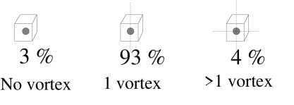
Figure 19: Percentages of monopole cubes pierced by zero, one, or more than one P-vortex lines, at $\beta=2.4$.

4.2 Field Collimation on 1-cubes

We define vortex limited Wilson loops $W_{n}(C)$ as the expectation value of Wilson loops on the full, unprojected lattice, subject to the the constraint that, on the projected lattice, exactly $n$ P-vortices pierce the minimal area of the loop (cf. [3]). We employ these gauge-invariant loop observables to probe the (a)symmetry of the color field around static monopoles, again at $\beta=2.4$.

Consider first, on a fixed time hypersurface, the set of all unit cubes which contain one static monopole, inside a cube pierced by a single P-vortex line. This means that two plaquettes on the cube are pierced by the vortex line, and four are not. The difference $S$ between the average plaquette $S_{0}$ on the lattice, and the plaquette on pierced/unpierced plaquettes of the monopole cube

$$S=S_{0}-<\frac{1}{2}\mbox{Tr}[UUU^{\dagger}U^{\dagger}]_{\mbox{cube face}}>$$ (4.1)

is shown in Fig. 20. For comparison, we have computed the same quantities in unit cubes, pierced by vortices, which do not contain any monopole current.

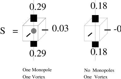
Figure 20: Excess plaquette action distribution on a monopole cube pierced by a single P-vortex. For comparison, the excess action distribution is also shown for a no-monopole cube pierced by a P-vortex.

It is obvious that the excess plaquette action associated with a monopole is extremely asymmetric, and almost all of it is concentrated in the P-vortex direction. Moreover, the action distribution around a monopole cube is not very different from the distribution on a cube pierced by a vortex, with no monopole at all inside. The two distributions are even more similar, if we make the additional restriction to “isolated” static monopoles; i.e. monopoles with no nearest-neighbor monopole currents. The excess action distribution for isolated monopoles, again compared to zero-monopole one-vortex cubes, is shown in Fig. 21.

Figure 21: Same as Fig. 20 for isolated monopoles.

4.3 Field Collimation on Larger Cubes

Finally we consider cubes which are $N$ lattice spacings on a side, in fixed-time hypersurfaces, having two faces pierced by a single P-vortex line and the other four faces unpierced. Again we restrict our attention to cubes containing either a single static monopole, or no monopole current. Each side of the cube is bounded by an $N\times N$ loop. Let

$$W_{1}^{M}(N,N) \equiv$$ 1-vortex loops, bounding a monopole N-cube

$$W_{0}^{M}(N,N) \equiv$$ 0-vortex loops, bounding a monopole N-cube

$$W_{1}^{0}(N,N) \equiv$$ 1-vortex loops, bounding a 0-monopole N-cube

$$W_{0}^{0}(N,N) \equiv$$ 0-vortex loops, bounding a 0-monopole N-cube (4.2)

denote the expectation value of $N\times N$ Wilson loops on 0/1-vortex faces of 0-monopole/1-monopole N-cubes. As a probe of the distribution of gauge-invariant flux around an N-cube, we compute the fractional deviation of these loops from $W_{0}^{0}(N,N)$ (which has the largest value) by

$$A^{M}_{0,1}={W^{0}_{0}(N,N)-W^{M}_{0,1}(N,N)\over W^{0}_{0}(N,N)}$$

$$A^{0}_{0,1}={W^{0}_{0}(N,N)-W^{0}_{0,1}(N,N)\over W^{0}_{0}(N,N)}$$ (4.3)

and of course $A^{0}_{0}=0$ by definition.

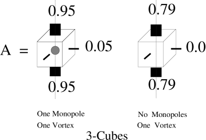
Figure 22: Gauge field collimation on a 3-cube pierced by a single P-vortex, for both one-monopole and no-monopole 3-cubes. $A$ is the fractional deviation of $W(3,3)$ on a cube face from the no-monopole, no-vortex value $W_{0}^{0}(3,3)$.

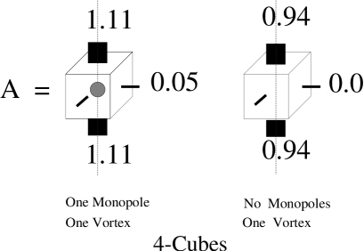
Figure 23: Same as Fig. 22, for 4-cubes.

The results, for $N=3$ cubes and $N=4$ cubes, are displayed in Figs. 22-23, with the actual values for the various loop types listed in Table 2. As with the excess-action distribution around a 1-cube, shown in Figs. 20-21, it is clear that gauge-invariant Wilson loop values are distributed very asymmetrically around a cube, and are strongly correlated with the direction of the P-vortex line. The presence or absence of a monopole inside the $N$-cube appears to have only a rather weak effect on the value of the loops around each side of the cube; the main variation is clearly due to the presence or absence of a vortex line piercing the side. Obviously, the strong correlation of loop values with vortex lines, and the relatively weak correlation of loop values with monopole current, fits the general picture discussed in the introduction, of confining flux collimated into tubelike structures.

(N)-cube $W_{1}^{M}(N,N)$ $W_{0}^{M}(N,N)$ $W_{1}^{0}(N,N)$ $W_{0}^{0}(N,N)$ 1-cube 0.3349 (10) 0.6007 (5) 0.4340 (5) 0.6472 (2) 2-cube 0.0599 (8) 0.2426 (5) 0.1101 (6) 0.2587 (3) 3-cube 0.0045 (7) 0.0825 (5) 0.0179 (5) 0.0864 (4) 4-cube -0.0030 (7) 0.0255 (7) 0.0016 (6) 0.0268 (5)

Table 2: Wilson loops on the faces of one-monopole ($W^{M}_{0,1}$) and zero monopole ($W^{0}_{0,1}$) N-cubes. The $0,1$ subscript refers to the number of P-vortices piercing the loop.

It seems clear that the gauge field-strength distribution around monopoles identified in maximal abelian gauge is highly asymmetric, and closely correlated to P-vortex lines, as one would naively guess from the picture shown in Fig. 1. This fact, by itself, doesn’t prove the vortex theory. One must admit the possibility that if the monopole positions were somehow held fixed, fluctuations in the direction of vortex lines passing through those monopoles might restore (on average) a Coulombic distribution. We therefore regard the findings in this section as fulfilling a necessary, rather than a sufficient, condition for the vortex theory to be correct. According to the vortex theory, confining fields are collimated along vortex lines, and this collimation should be visible on the lattice in some way, e.g. showing up in spatially asymmetric distributions of Wilson loop values. This strong asymmetry is, in fact, what we find on the lattice.

5 The Seiberg-Witten confinement scenario and
$Z_{2}$-fluxes

The beautiful description of confinement by monopoles when $N\!\!=\!2$ supersymmetric Yang-Mills theory is softly broken to $N\!\!=\!1$ supersymmetric Yang-Mills theory has enhanced the impression that the mechanism for confinement in pure Yang-Mills theory is monopole condensation. Above we have provided evidence that it is in fact $Z_{2}$ fluctuations which are responsible for confinement in Yang-Mills theory even on abelian-projected lattices; see refs. [3, 4] for the evidence on the full, unprojected lattices. As regards the $N\!\!=\!2$ supersymmetric Yang-Mills theory softly broken to $N\!\!=\!1$, we would simply argue that the approximate low-energy effective theory of Seiberg and Witten is not able describe all aspects of confinement at sufficiently large distance scales. In particular, the low-energy effective theory cannot explain the perimeter law of double-charged Wilson loops.

It may be useful here to make a distinction between the full effective action, obtained by integrating out all massive fields, and the “low-energy” effective action, which neglects all non-local or higher-derivative terms in the full effective action. The Seiberg-Witten calculation was aimed at determining the low-energy effective action of the softly broken $N\!\!=\!2$ theory. However, in a confining theory, non-local terms induced by massive fields can have important effects at long distances.

The relation between the Seiberg-Witten theory and pure Yang-Mills theory in four dimensions has many similarities to the relation between the Georgi-Glashow model and pure Yang-Mills theory in three dimensions. In both theories the presence of a Higgs field is of utmost importance for the existence of monopoles. In the Georgi Glashow model it is the existence of a monopole condensate which is responsible for the mass of the (dual) photon and for confinement of the smallest unit of electric $U(1)$ charge. However, as emphasized in [6], the effective low energy Coulomb gas picture of monopoles does not explain the fact that double-charged Wilson loops follow a perimeter law rather than an area law. The reason is that in a confining theory there is not equivalence between low-energy and long-distance physics. At sufficiently long distance it will always be energetically favorable to excite charged massive $W$-fields and screen $q=$ even external charges, thus preventing a genuine string tension between such charges. At these large scales, a description in terms of U(1)-disordering configurations (the monopole Coulomb gas) breaks down, and a description in terms of $Z_{2}$ disorder must take over. As shown in [6] the range of validity of the monopole Coulomb gas picture decreases as the mass of the $W$-field decreases, and, in the limit of an unbroken $SU(2)$ symmetry, confinement can only be described adequately in terms of $Z_{2}$ fluctuations.

In the Seiberg-Witten theory, $N\!\!=\!2$ supersymmetry ensures that the Higgs vacuum is parameterized by an order parameter $u=\left\langle{\rm Tr}\,\phi^{2}\right\rangle$ corresponding to the breaking of $SU(2)$ to $U(1)$. For large values of $u$ we have a standard scenario: at energy scales $\mu\gg\sqrt{u}$ all field theoretical degrees of freedom contribute to the $\beta$-function, which corresponds to the asymptotically free theory. For energies lower than $\sqrt{u}$ only the $U(1)$ part of the theory is effective. In these considerations the dynamical confinement scale

$$\Lambda_{N=2}^{4}=\mu^{4}\exp(-8\pi^{2}/g(\mu)^{2})$$

obtained by the one-loop perturbative calculation plays no role. The remarkable observation by Seiberg and Witten was that even when $u\leq\Lambda^{2}_{N=2}$, where one would naively expect that non-Abelian dynamics was important, the system remains in the $U(1)$ Coulomb phase due to supersymmetric cancellations of non-Abelian quantum fluctuations. As $u$ decreases the effective electric charge associated with the unbroken $U(1)$ part of $SU(2)$ increases, while the masses of the solitonic excitations which are present in the theory, will decrease. Dictated by monodromy properties of the so-called prepotential of the effective low energy Lagrangian, the monopoles become massless at a point $u\sim\Lambda^{2}_{N=2}$ where the effective electric charge has an infrared Landau pole and diverges. However, in the neighborhood of $u\sim\Lambda^{2}_{N=2}$, this strongly coupled theory has an effective Lagrangian description as a weakly coupled theory when expressed in terms of dual variables, namely a monopole hyper-multiplet and a dual photon vector multiplet. The perturbative coupling constant is now $g_{D}=4\pi/g$ and the point where monopoles condense corresponds to $g_{D}=0$.

A remarkable observation of Seiberg and Witten is that the breaking of $N\!\!=\!2$ to $N\!\!=\!1$ supersymmetry by adding a mass term superpotential will generate a mass gap, originating from a condensation of the monopoles. By the dual Meissner effect this theory confines the electric $U(1)$ charge at distances larger than the inverse $N\!\!=\!2$ symmetry breaking scale. In terms of the underlying microscopic theory it is believed that the reduction of symmetry from $N\!\!=\!2$ to $N\!\!=\!1$ allows excitations closer to generic non-supersymmetric “confinement excitations”, but that the soft breaking ensures that the theory is still close enough to the $N\!\!=\!2$ to remain an effective $U(1)$ theory. Thus we see that in the Seiberg-Witten scenario we can, by introducing the mass term superpotential, describe a $U(1)$ confining-deconfining transition from the $N\!\!=\!2$ Coulomb phase to the $N\!\!=\!1$ confining phase.

But precisely as for the Georgi-Glashow model, the monopole condensate picture for the $N=1$ confining theory is incomplete in the sense that it cannot describe the obvious fact that double-charged Wilson loops will have a perimeter law rather than an area law. Clearly, $q=$ even external charges can be screened by the massive charged $W$-fields in the softly broken $N=2$ supersymmetric Yang-Mills theory, a fact which has profound implications for the large-scale structure of confining fluctuations. But neither the non-local effects of the $W$-fields, nor the $W$-fields themselves, appear in the low energy effective action, a fact which illustrates once more that long distance physics is not captured by the (local) low energy effective action in a confining theory.

6 Discussion

A point which was stressed both in ref. [6] and in the last section (see also [25]), and which is surely relevant to the results reported here, is that charged fields in a confining theory can have a profound effect on the far-infrared structure of the theory, even if those fields are very massive. As an obvious example, consider integrating out the quark fields in QCD, to obtain an effective pure gauge theory. This effective pure gauge theory does not produce an asymptotic area law falloff for Wilson loops, which means that confining field configurations are somehow suppressed at large distances. A second example is the Georgi-Glashow model in D=3 dimensions ($GG_{3}$), as discussed in ref. [6]. In this case the W-bosons are massive, and if their effects at large scales are simply ignored, then the model would be essentially equivalent to the theory of photons and monopoles, i.e. a monopole Coulomb gas, analyzed many years ago by Polyakov [7]. In the monopole Coulomb gas, all multiples of the elementary electric charge are confined; but this is not what actually happens in the Georgi-Glashow model. The reason is that W-bosons are capable of screening even multiples of electric charge, which means that even-charge Wilson loops fall only with a perimeter law, and even-charge Polyakov lines have finite vacuum expectation values in the confined phase. If we again imagine integrating out the W and Higgs fields, then the effective abelian theory confines only odd multiples of charge, the global symmetry is $Z_{2}$, rather than U(1), and the theory is clearly not equivalent to either a monopole Coulomb gas, or to compact $QED_{3}$. If one asks: how can the effective long-range theory, which involves only the photon field, be anything different from compact $QED_{3}$, the answer is that the integration over W and Higgs fields produces non-local terms in the effective action. We note, once again, that charged fields in a confining theory have very long-range effects. The fact that these fields are massive does not imply that they can only lead, in the effective abelian action, to local terms, or that the non-local terms can be neglected at large scales. These remarks also apply to the Seiberg-Witten model, as discussed in the last section.

In this article we have concentrated largely on a third example: abelian-projected Yang-Mills theory in maximal abelian gauge. Calculations on the abelian-projected lattice can be always regarded as being performed in an effective abelian theory, obtained by integrating out the off-diagonal gluon fields (and ghosts) in the given gauge. It is often argued that the off-diagonal gluon fields are massive, and therefore do not greatly affect the long-range structure of the theory. The long-range structure, according to that view, is dominated exclusively by the diagonal gauge fields (the “photons”) and the corresponding abelian monopoles, which together are equivalent to a Coulomb gas of monopoles (D=3) or monopole loops (D=4). Then, since only abelian fields are involved, the global symmetry of the effective long-range theory is expected to be U(1), and all multiples of abelian charge are confined. We have seen that reasoning of this sort, which neglects the long-distance effects of massive charged fields, can lead to erroneous conclusions. In fact, we have found that on the abelian projected lattice:

• Confinement of all multiples of abelian charge does not occur on the abelian-projected lattice; charge $q=2$ Polyakov lines have a non-zero VEV.

• As a result, the global symmetry of the abelian-projected lattice is at most $Z_{2}$, rather than U(1).

• Monopole dominance breaks down rather decisively, at least when applied to charge $q=2$ operators.

• The distribution of Wilson loop values is highly asymmetric on an N-cube. There is a very strong correlation between loop values and the P-vortex direction, but only a rather weak correlation with the presence or absence of a static monopole in the N-cube.

In addition, in the usual maximal abelian gauge, there is a breakdown of positivity, which is surely due to the absence of a transfer matrix in this gauge. The loss of positivity can be avoided (at the cost of rotation invariance) by going to a spacelike maximal abelian gauge, where we again find $q=2$ string-breaking and deconfinement. The picture of a U(1)-symmetric monopole Coulomb gas or dual superconductor, confining all multiples of the elementary abelian charge, is clearly not an adequate description of the abelian-projected theory at large distance scales. On the other hand, the results reported here fit quite naturally into the vortex picture, where confining magnetic flux on the projected lattice is collimated in units of $\pm\pi$.

The center vortex theory has a number of well-known (and gauge-invariant) virtues. In particular, the vortex mechanism is the natural way to understand, in terms of vacuum gauge-field configurations, the screening of color charges in zero N-ality representations, as well the loss of $Z_{N}$ global symmetry in the deconfinement phase transition [30]. Center vortex structure is visible on unprojected lattices, through the correlation of P-vortex location with gauge-invariant observables [3, 4]. The evidence we have reported here, indicating vortex structure on large scales even on abelian-projected lattices, increases our confidence that center vortices are essential to the mechanism of quark confinement.

Acknowledgements

J.Gr. is happy to acknowledge the hospitality of the theory group at Lawrence Berkeley National Laboratory, where some of this work was carried out. J.Gr.’s research is supported in part by the U.S. Department of Energy under Grant No. DE-FG03-92ER40711.

Appendix A Appendix

In this Appendix we present the detailed argument, outlined in section 3, that $\overline{\theta}^{ph}_{I}=-\overline{\theta}^{ph}_{II}$ and $P_{1}<0$ in the additive $\theta^{\prime}=\theta+\theta^{M}$ configurations.

The approximation used here is to ignore, at fixed $\theta_{M}$, the fluctuctions of $\theta^{ph}$ around the mean value $\overline{\theta}^{ph}(\theta^{M})$; i.e. the vev of any periodic function $F(\theta)$ of the Polyakov phase $\theta$

$$<F>=\int^{\pi}_{-\pi}d\theta~{}F(\theta){\cal P}(\theta)$$ (A.1)

is approximated by

$$<F>=\int^{\pi}_{-\pi}d\theta^{M}{1\over 2\pi}F(\theta^{M}+\overline{\theta}^{ph}(\theta^{M}))$$ (A.2)

where the factor of $1/2\pi$ corresponds to the uniform probability distribution for $\theta^{M}$. The mean value $\overline{\theta}^{ph}(\theta^{M})$ is defined as

$$\overline{\theta}^{ph}(\theta^{M}) = {1\over Z_{\theta^{M}}}\int D\theta_{\mu}(x)~{}\arg\left(P_{1}(\vec{x})e^{-i\theta^{M}}\right)\delta\left[P_{M1}(\vec{x}),e^{i\theta^{M}}\right]e^{-S_{eff}}$$

$$Z_{\theta^{M}} = \int D\theta_{\mu}(x)~{}\delta\left[P_{M1}(\vec{x}),e^{i\theta^{M}}\right]e^{-S_{eff}}$$ (A.3)

where

$$P_{1}(\vec{x}) = \prod_{n=1}^{N_{T}}\exp[i\theta_{4}(\vec{x}+n\hat{4})]$$

$$P_{M1}(\vec{x}) = \prod_{n=1}^{N_{T}}\exp[i\theta^{M}_{4}(\vec{x}+n\hat{4})]$$ (A.4)

are Polyakov lines in the abelian and MD lattices, and $S_{eff}$ is the effective abelian action, obtained after integrating out all off-diagonal gluons and ghost fields. Due to translation invariance, $\overline{\theta}^{ph}(\theta^{M})$ does not depend on the particular spatial position $\vec{x}$ chosen in (A.3).

From its definition, $\overline{\theta}^{ph}(\theta^{M})$ is obviously periodic w.r.t. $\theta^{M}\rightarrow\theta^{M}+2\pi$. It is also an odd function of $\theta^{M}$, i.e.

$$\overline{\theta}^{ph}(\theta^{M})=-\overline{\theta}^{ph}(-\theta^{M})$$ (A.5)

This is derived by first noting that the $\theta^{M}_{\mu}(x)$ link angles are functions of the $\theta_{\mu}(x)$ link angles according to eqs. (2.5)-(2.7), and that $\theta^{M}_{\mu}(x)\rightarrow-\theta^{M}_{\mu}(x)$ under the transformation $\theta_{\mu}(x)\rightarrow-\theta_{\mu}(x)$. Then, making the change of variables $\theta_{\mu}(x)\rightarrow-\theta_{\mu}(x)$ in the integral (A.3), we have

$$Z_{\theta^{M}} = \int D\theta_{\mu}(x)~{}\delta\left[P^{*}_{M1}(\vec{x}),e^{i\theta^{M}}\right]e^{-S_{eff}}$$ (A.6)

$$= \int D\theta_{\mu}(x)~{}\delta\left[P_{M1}(x),e^{-i\theta^{M}}\right]e^{-S_{eff}}$$

$$= Z_{-\theta^{M}}$$

and

$$\overline{\theta}^{ph}(\theta^{M}) = {1\over Z_{\theta}^{M}}\int D\theta_{\mu}(x)\mbox{arg}\left(P^{*}_{1}(x)e^{-i\theta^{M}}\right)\delta\left[P^{*}_{M1}(x),e^{i\theta^{M}}\right]e^{-S_{eff}}$$ (A.7)

$$= {1\over Z_{-\theta^{M}}}\int D\theta_{\mu}(x)(-1)\times\mbox{arg}\left(P_{1}(x)e^{i\theta^{M}}\right)\delta\left[P_{M1}(x),e^{-i\theta^{M}}\right]e^{-S_{eff}}$$

$$= -\overline{\theta}^{ph}(-\theta^{M})$$

The fact that $\overline{\theta}^{ph}(\theta^{M})$ is an odd function of $\theta^{M}$, combined with $2\pi$-periodicity, gives us

$$\overline{\theta}^{ph}(\pi)=\overline{\theta}^{ph}(-\pi)=\overline{\theta}^{ph}(0)=0$$ (A.8)

We now define the variable

$$\overline{\theta}(\theta^{M})\equiv\theta^{M}+\overline{\theta}^{ph}(\theta^{M})$$ (A.9)

which is the average Polyakov phase at fixed $\theta^{M}$. It will be assumed that $\overline{\theta}(\theta^{M})$ is a single-valued function of $\theta^{M}$. Eq. (A.9) can then be inverted to define $\theta^{M}$ implicitly as a function of $\overline{\theta}$

$$\theta^{M}(\overline{\theta})=\overline{\theta}-\overline{\theta}^{ph}[\theta^{M}(\overline{\theta})]$$ (A.10)

and it will be convenient to introduce the notation

$$\overline{\theta}^{ph}[\overline{\theta}]\equiv\overline{\theta}^{ph}[\theta^{M}(\overline{\theta})]$$ (A.11)

Applying the change of variable (A.9) to eq. (A.2), we have

$$<F>=\int^{\pi}_{-\pi}d\overline{\theta}~{}{1\over 2\pi}{d\theta^{M}\over d\overline{\theta}}F(\overline{\theta})$$ (A.12)

where, from eqs. (A.8) and (A.9), we see that the limits of integrations are unchanged. Comparing (A.12) to (A.1), the Polyakov phase probability distribution ${\cal P}(\theta)$ can be identified with

$${\cal P}(\overline{\theta}) = {1\over 2\pi}{d\theta^{M}\over d\overline{\theta}}$$ (A.13)

$$= {1\over 2\pi}\left(1-{d\overline{\theta}^{ph}\over d\overline{\theta}}\right)$$

in the approximation (A.2).

Assuming $Z_{2}$ symmetry in the confined phase, we have from eq. (1.10)

$${\cal P}(\overline{\theta})={1\over 2\pi}\left(1+2\sum_{q=\mbox{even}}P_{q}\cos(q\overline{\theta})\right)$$ (A.14)

which means that ${\cal P}(\overline{\theta})$ is even w.r.t. reflections around $\overline{\theta}=0,\pm{\pi\over 2}$; i.e.

$${\cal P}(\pi-\overline{\theta}) = {\cal P}(\overline{\theta})$$

$${\cal P}(-\pi-\overline{\theta}) = {\cal P}(\overline{\theta})$$

$${\cal P}(-\overline{\theta}) = {\cal P}(\overline{\theta})$$ (A.15)

Comparing eq. (A.15) with (A.13), we find that ${d\overline{\theta}^{ph}/d\overline{\theta}}$ is also even under reflections around $\overline{\theta}=0,\pm{\pi\over 2}$. Since the derivative of an odd function is an even function, this means that

$$\overline{\theta}^{ph}[\overline{\theta}]=a+\phi(\overline{\theta})$$ (A.16)

where $\phi(\overline{\theta})$ is odd under reflections around $\overline{\theta}=0$, and $a$ is a constant. However, since

$$\overline{\theta}(\theta^{M}=0)=\overline{\theta}^{ph}(0)=0$$ (A.17)

it follows that $\overline{\theta}^{ph}[\overline{\theta}=0]=\overline{\theta}^{ph}(\theta^{M}=0)=0$. Then $a=0$, and $\overline{\theta}^{ph}[\overline{\theta}]$ is odd around $\overline{\theta}=0$. Further, from (A.8), (A.9), and the assumed single-valuedness of $\overline{\theta}(\theta^{M})$, it follows that $\theta^{M}(\overline{\theta}=\pm\pi)=\pm\pi$, and therefore that

$$\overline{\theta}^{ph}[\pm\pi]=0$$ (A.18)

Then, since $\overline{\theta}^{ph}[0]=\overline{\theta}^{ph}[\pi]=0$, and ${d\overline{\theta}^{ph}/d\overline{\theta}}$ is even w.r.t. reflections around ${\pi\over 2}$, it follows that $\overline{\theta}^{ph}[{\pi\over 2}]=0$, and that $\overline{\theta}^{ph}[\overline{\theta}]$ is odd w.r.t. reflections around ${\pi\over 2}$. By the same reasoning, $\overline{\theta}^{ph}[\overline{\theta}]$ is also odd w.r.t. reflections around $-{\pi\over 2}$. To summarize, $\overline{\theta}^{ph}[\overline{\theta}]$ has the reflection properties:

$$\overline{\theta}^{ph}[-\overline{\theta}] = -\overline{\theta}^{ph}[\overline{\theta}]$$

$$\overline{\theta}^{ph}[\pi-\overline{\theta}] = -\overline{\theta}^{ph}[\overline{\theta}]$$

$$\overline{\theta}^{ph}[-\pi-\overline{\theta}] = -\overline{\theta}^{ph}[\overline{\theta}]$$ (A.19)

where the last two relationships are a consequence of global $Z_{2}$ symmetry in the confined phase. Therefore

$$\overline{\theta}^{ph}_{I} = {2\over\pi}\int_{0}^{\pi/2}d\theta^{M}~{}\overline{\theta}^{ph}(\theta^{M})$$ (A.20)

$$= 4\int_{0}^{\pi/2}d\overline{\theta}~{}{\cal P}(\overline{\theta})\overline{\theta}^{ph}[\overline{\theta}]$$

$$= 4\int_{\pi/2}^{\pi}d\overline{\theta}~{}{\cal P}(\pi-\overline{\theta})\overline{\theta}^{ph}[\pi-\overline{\theta}]$$

$$= -4\int_{\pi/2}^{\pi}d\overline{\theta}~{}{\cal P}(\overline{\theta})\overline{\theta}^{ph}[\overline{\theta}]$$

$$= -{2\over\pi}\int_{\pi/2}^{\pi}d\theta^{M}~{}\overline{\theta}^{ph}(\theta^{M})$$

$$= -\overline{\theta}^{ph}_{II}$$

This explains why the correlation between $\theta^{ph}$ and $\theta^{M}$ found numerically in eq. (3.4) is a consequence of global $Z_{2}$ invariance.

Our second task is to understand why $P_{1}$ is negative in the $\theta^{\prime}=\theta+\theta^{M}$ additive configuration, given that ${\cal P}(\theta)$ is peaked around $\theta={\pi\over 2}$ as discussed in section 3. Introducing the probability distribution ${\cal P}^{\prime}(\theta^{\prime})$ for the Polyakov phases in the additive configurations

$$<F(\overline{\theta}^{\prime})>=\int^{\pi}_{-\pi}d\overline{\theta}^{\prime}~{}F(\overline{\theta}^{\prime}){\cal P}^{\prime}(\overline{\theta}^{\prime})$$ (A.21)

and again neglecting the fluctuations of $\theta^{ph}$ at fixed $\theta^{M}$ around the mean $\overline{\theta}^{ph}(\theta^{M})$,

$$<F>=\int^{\pi}_{-\pi}d\theta^{M}{1\over 2\pi}F(2\theta^{M}+\overline{\theta}^{ph}(\theta^{M}))$$ (A.22)

Under the change of variables

$$\overline{\theta}^{\prime}=2\theta^{M}+\overline{\theta}^{ph}(\theta^{M})$$ (A.23)

eq. (A.22) becomes

$$<F>=\int^{2\pi}_{-2\pi}d\overline{\theta}^{\prime}{1\over 2\pi}{d\theta^{M}\over d\overline{\theta}^{\prime}}F(\overline{\theta}^{\prime})$$ (A.24)

The limits of integration have changed, but the original limits can be restored using the $2\pi$-periodicity of the integrand. To demonstrate the periodicity, we first have

$$\overline{\theta}^{\prime}(\overline{\theta}+\pi) = \overline{\theta}+\pi+\theta^{M}(\overline{\theta}+\pi)$$ (A.25)

$$= \overline{\theta}+\pi+(\overline{\theta}+\pi-\overline{\theta}^{ph}[\overline{\theta}+\pi])$$

$$= \overline{\theta}+\pi+(\overline{\theta}+\pi+\overline{\theta}^{ph}[-\overline{\theta}])$$

$$= \overline{\theta}+\pi+(\overline{\theta}+\pi-\overline{\theta}^{ph}[\overline{\theta}])$$

$$= \overline{\theta}^{\prime}(\overline{\theta})+2\pi$$

where the reflection properties (A.19) have been used. Single-valuedness of $\overline{\theta}^{\prime}(\overline{\theta})$ then implies the converse property

$$\overline{\theta}(\overline{\theta}^{\prime}+2\pi)=\overline{\theta}(\overline{\theta}^{\prime})+\pi$$ (A.26)

Next,

$${d\theta^{M}\over d\overline{\theta}^{\prime}} = {d\theta^{M}\over d\overline{\theta}}{d\overline{\theta}\over d\overline{\theta}^{\prime}}$$ (A.27)

$$= \left(1-{d\overline{\theta}^{ph}\over d\overline{\theta}}\right)\left(2-{d\overline{\theta}^{ph}\over d\overline{\theta}}\right)^{-1}$$

Then, applying (A.26) plus the fact that $d\overline{\theta}^{ph}/d\overline{\theta}$ is even w.r.t. reflections $\overline{\theta}\rightarrow-\overline{\theta}$ and $\overline{\theta}\rightarrow\pi-\overline{\theta}$,

$$\left({d\theta^{M}\over d\overline{\theta}^{\prime}}\right)_{\overline{\theta}^{\prime}+2\pi} = \left(1-{d\overline{\theta}^{ph}\over d\overline{\theta}}\right)_{\overline{\theta}(\overline{\theta}^{\prime})+\pi}\left(2-{d\overline{\theta}^{ph}\over d\overline{\theta}}\right)_{\overline{\theta}(\overline{\theta}^{\prime})+\pi}^{-1}$$ (A.28)

$$= \left(1-{d\overline{\theta}^{ph}\over d\overline{\theta}}\right)_{-\overline{\theta}(\overline{\theta}^{\prime})}\left(2-{d\overline{\theta}^{ph}\over d\overline{\theta}}\right)_{-\overline{\theta}(\overline{\theta}^{\prime})}^{-1}$$

$$= \left(1-{d\overline{\theta}^{ph}\over d\overline{\theta}}\right)_{\overline{\theta}(\overline{\theta}^{\prime})}\left(2-{d\overline{\theta}^{ph}\over d\overline{\theta}}\right)_{\overline{\theta}(\overline{\theta}^{\prime})}^{-1}$$

Since $F(\overline{\theta}^{\prime})$ is periodic by definition, this establishes the $2\pi$-periodicity of the integrand in (A.24), which can then be written

$$<F> = \int^{\pi}_{-\pi}d\overline{\theta}^{\prime}{1\over\pi}{d\theta^{M}\over d\overline{\theta}^{\prime}}F(\overline{\theta}^{\prime})$$ (A.29)

$$= \int^{\pi}_{-\pi}d\overline{\theta}^{\prime}{1\over\pi}\left(1-{d\overline{\theta}^{ph}\over d\overline{\theta}}\right)\left(2-{d\overline{\theta}^{ph}\over d\overline{\theta}}\right)^{-1}F(\overline{\theta}^{\prime})$$

Comparing (A.29) with (A.21)

$${\cal P}(\overline{\theta}^{\prime})={1\over\pi}\left(1-{d\overline{\theta}^{ph}\over d\overline{\theta}}\right)\left(2-{d\overline{\theta}^{ph}\over d\overline{\theta}}\right)^{-1}$$ (A.30)

Single-valuedness of $\theta^{M}(\overline{\theta})$ implies that $d\overline{\theta}^{ph}/d\overline{\theta}<1$, and with this restriction ${\cal P}(\overline{\theta}^{\prime})$ is a maximum where $d\overline{\theta}^{ph}/d\overline{\theta}$ is a minimum. However, we have previously deduced from the the fact that $P_{1}=0$ and $P_{2}<0$ that the probability distribution

$${\cal P}(\overline{\theta})=1-{d\overline{\theta}^{ph}\over d\overline{\theta}}$$ (A.31)

is $Z_{2}$ invariant and peaked at $\overline{\theta}=\pm\pi/2$. Again, this distribution is maximized when $d\overline{\theta}^{ph}/d\overline{\theta}$ is minimized, which implies that $d\overline{\theta}^{ph}/d\overline{\theta}$ is a minimum at $\overline{\theta}=\pm\pi/2$. Finally,

$$\overline{\theta}^{\prime}\left(\overline{\theta}=\pm{\pi\over 2}\right) = {\pi\over 2}+\theta^{M}\left(\overline{\theta}={\pi\over 2}\right)$$ (A.32)

$$= {\pi\over 2}+\left({\pi\over 2}-\overline{\theta}^{ph}[{\pi\over 2}]\right)$$

$$= \pi$$

As a consequence, $d\overline{\theta}^{ph}/d\overline{\theta}$ is minimized at $\overline{\theta}^{\prime}=\pi$ (and also, by the same arguments, at $\overline{\theta}^{\prime}=-\pi$), which means that ${\cal P}(\overline{\theta}^{\prime})$ is peaked at $\overline{\theta}^{\prime}=\pm\pi$, as illustrated in Fig. 15. This explains why we expect $P_{1}<0$ in the additive configuration.

References

-
[1]
G. ’t Hooft, Nucl. Phys. B138 (1978) 1,
G. Mack, in Recent Developments in Gauge Theories, edited by G. ’t Hooft et al. (Plenum, New York, 1980)
J. M. Cornwall, Nucl. Phys. B157 (1979) 392
H. B. Nielsen and P. Olesen, Nucl. Phys. B160 (1979) 380;
J. Ambjørn and P. Olesen, Nucl. Phys. B170 (1980) 60; 265;
J. Ambjørn, B. Felsager, and P. Olesen, Nucl. Phys. B175 (1980) 349;
R. P. Feynman, Nucl. Phys. B188 (1981) 479. - [2] G. ’t Hooft, Nucl. Phys. B190 [FS3] (1981) 455.
- [3] L. Del Debbio, M. Faber, J. Giedt, J. Greensite, and Š. Olejník, Phys. Rev. D58 (1998) 094501, hep-lat/9801027.
- [4] Ph. de Forcrand and M. D’Elia, Phys. Rev. Lett. 82 (1999) 4582, hep-lat/9901020.
- [5] L. Del Debbio, M. Faber, J. Greensite, and Š. Olejník, in New Developments in Quantum Field Theory, ed. Poul Henrik Damgaard and Jerzy Jurkiewicz (Plenum Press, New York–London, 1998) 47, hep-lat/9708023.
- [6] J. Ambjørn and J. Greensite, JHEP (1998) 9805:004, hep-lat/9804022.
- [7] A. Polyakov, Nucl. Phys. B120 (1977) 429.
- [8] M. Zach, M. Faber, and P. Scala, Nucl. Phys. B529 (1998) 505, hep-lat/9709017.
- [9] A. Hart and M. Teper, hep-lat/9902031.
- [10] M. Chernodub, S. Kato, N. Nakamura, M. Polikarpov, and T. Suzuki, hep-lat/9902013.
- [11] L. Del Debbio, M. Faber, J. Giedt, J. Greensite, and Š. Olejník, Nucl. Phys. Proc. Suppl. 53 (1997) 141, hep-lat/9607053.
-
[12]
H. Shiba and T. Suzuki, Phys. Lett. B333 (1994) 461,
hep-lat/9404015;
J. Stack, S. Nieman, and R. Wensley, Phys. Rev. D50 (1994) 3399, hep-lat/9404014. - [13] T. De Grand and D. Toussaint, Phys. Rev. D22 (1980) 2473.
- [14] P. Stephenson, Nucl. Phys. B550 (1999) 427, hep-lat/9902002.
- [15] O. Philipsen and H. Wittig, Phys. Lett. B451 (1999) 146, hep-lat/9902003.
- [16] C. Michael, Nucl. Phys. B Proc. Suppl. 26 (1992) 417.
- [17] M. Faber, J. Greensite, and Š. Olejník, Phys. Rev. D57 (1998) 2603, hep-lat/9710039.
- [18] M. Faber, J. Greensite, and Š. Olejník, Acta. Phys. Slov. 49 (1999) 177, hep-lat/9807008.
- [19] G. Poulis, Phys. Rev. D54 (1996) 6974, hep-lat/9601013.
- [20] G. Bali et al., Phys. Rev. D54 (1996) 2863, hep-lat/9603012.
- [21] T. Suzuki et al., Phys. Lett. B347 (1995) 375, hep-lat/9408003.
- [22] M. Chernodub, M. Polikarpov, and A. Veselov, JETP Lett. 69 (1999) 174, hep-lat/9812012.
- [23] A. Hart and M. Teper, Phys. Rev. D58 (1998) 014504, hep-lat/9712003.
- [24] L. Del Debbio, M. Faber, J. Greensite, and Š. Olejník, Phys. Rev. D55 (1997) 2298, hep-lat/9610005.
- [25] G. Bali, hep-ph/9809351.
- [26] J. Ambjørn, D. Espriu, N. Sasakura, Mod.Phys.Lett. A12 (1997) 2665; Fortsch.Phys. 47 (1999) 287.
- [27] N. Evans, S.D.H. Hsu and M. Schwetz, Phys. Lett. B355 (1995) 475. N. Evans, S.D.H. Hsu, M. Schwetz and S.B. Selipsky, Nucl. Phys. B456 (1995) 205. N. Evans, S.D.H. Hsu and M. Schwetz, Nucl. Phys. B484 (1997) 124; Controlled Soft Breaking of N=1 SQCD, hep-th/9703197.
- [28] L. Alvarez-Gaumé, J. Distler, C. Kounnas and M. Mariño, Int. J. Mod. Phys. A11 (1996) 4745. L. Alvarez-Gaumé and M. Mariño, Int. J. Mod. Phys. A12 (1997) 975. L. Alvarez-Gaumé, M. Mariño and F. Zamora, Softly Broken QCD with Massive Quark Hypermultiplets I, II, hep-th/9703072, 9707017.
- [29] O. Aharony, J. Sonnenschein, M.E. Peskin and S. Yankielowicz, Phys. Rev. D52 (1995) 6157. E. D’Hoker, Y. Mimura and N. Sakai, Phys. Rev. D54 (1996) 7724. K. Konishi, Phys. Lett. B392 (1997) 101. K. Konishi and H. Terao, CP, Charge Fractionalizations and Low Energy Effective Actions in the SU(2) Seiberg-Witten Theories with Quarks, hep-th/9707005.
-
[30]
M. Engelhardt, K. Langfeld, H. Reinhardt, and O. Tennert,
hep-lat/9904004; and Phys. Lett. B452 (1999) 301, hep-lat/9805002;
R. Bertle, M. Faber, J. Greensite, and Š. Olejník, JHEP 9903 (1999) 019, hep-lat/9903023.