Universal Scaling of the Chiral Condensate
in Finite-Volume Gauge Theories

Abstract

We confront exact analytical predictions for the finite-volume scaling of the chiral condensate with data from quenched lattice gauge theory simulations. Using staggered fermions in both the fundamental and adjoint representations, and gauge groups SU(2) and SU(3), we are able to test simultaneously all of the three chiral universality classes. With overlap fermions we also test the predictions for gauge field sectors of non-zero topological charge. Excellent agreement is found in most cases, and the deviations are understood in the others.

I Introduction

The constraints imposed by chiral symmetry breaking in gauge theories can be surprisingly strong. Low-energy theorems, the dynamics of pseudo-Goldstone bosons in an expansion around the zero-momentum limit, and the whole framework of effective chiral Lagrangians are examples of this. Generally these constraints are imposed on the effective low-energy degrees of freedom only. It is much more surprising that both spontaneous chiral symmetry breaking and the explicit breaking of chiral symmetry due to the U(1) anomaly also can be used to give exact analytical predictions for the underlying fermion degrees of freedom. This is possible when one restricts the gauge theory to a large but finite four-volume $V$ obeying the inequality [1]

$$V~{}<<~{}\frac{1}{m_{\pi}^{4}}~{},$$ (1)

where $m_{\pi}$ is the pseudo-Goldstone mass. In this rather extreme limit the QCD partition function depends on the fermion masses $m_{i}$ only in the particular combination $\mu_{i}\equiv V\Sigma m_{i}$, where $\Sigma$ is the chiral condensate. While the four-volume $V$ must be taken to infinity in order to obtain analytical predictions, a finite-size scaling regime is thus achieved by sending fermion masses $m_{i}$ to zero at just such a rate that the $\mu_{i}$’s remain fixed. This is an exact finite-size scaling region in the same sense as near critical points: we can reach as accurate agreement we wish by simply choosing a sufficiently large four-volume $V$. In contrast to what one is accustomed to in statistical mechanics, the finite-size scaling functions are in this case known exactly, both in shape and absolute normalization, once one has the value of the infinite-volume chiral condensate $\Sigma$.

One of the remarkable aspects of the finite-size scaling region (1) is its relation to Random Matrix Theory results that have proven to be universal [2, 3, 4]. There is a beautiful classification of the possible chiral symmetry breaking patterns for different gauge groups and color representations of the fermions in terms of the classical Random Matrix Theory ensembles labeled by the so-called Dyson index. This leads to three major universality classes [5]. For the quenched case, the analytical prediction for the mass-dependent chiral condensate was in fact first obtained by Verbaarschot [6] using the exact formula for the microscopic Dirac operator spectrum as derived from Random Matrix Theory. It has later become clear that these results can also be derived from finite-volume partition functions alone [7]. A powerful analytical technique uses fully or partially quenched (supersymmetric) chiral Lagrangians [8]. Lattice gauge simulations have already shown nice agreement with the exact analytical predictions for the microscopic Dirac operator spectrum associated with all three different universality classes [9, 10, 11] using staggered fermions. It has been particularly challenging to see also the detailed analytical predictions in gauge field sectors of fixed non-zero topological charge $\nu$, and this has very recently been achieved using perfect actions [12] and overlap fermions [13].

The purpose of this paper is to perform a systematic series of lattice gauge theory tests of the exact predictions related to the mass-dependent chiral condensates and one of the chiral susceptibilities. For the case of gauge group SU(3) and staggered fermions in the fundamental representation such an analysis was first performed [6] on the basis of lattice gauge theory data from the Columbia group [14]. These data, based on configurations with $N_{f}=2$ dynamical fermions, were taken for finite-temperature lattice volumes, and with rather large correlation lengths. Because the dynamical fermion masses were large on that scale, and the physical pions therefore not obeying the inequality (1), the configurations were in fact to be considered as completely quenched on the scale of the mass of the valence fermions. As there are very accurate estimates for the infinite-volume chiral condensate $\Sigma$ for the same theory at different $\beta$-values [10], we now have parameter-free predictions at these $\beta$-values. Furthermore, we can probe much larger physical volumes (and hence obtain higher accuracy), and our result will not be contaminated by finite-temperature effects. This case corresponds to the chiral unitary (chUE) Random Matrix Theory ensemble. We next turn to gauge group SU(2) and staggered fermions in the fundamental and adjoint representations. The former case corresponds at our finite lattice spacings to the chiral symplectic ensemble (chSE) in the Random Matrix Theory classification, while the latter corresponds to the chiral orthogonal ensemble (chOE). In this way we cover all three major universality classes. However, staggered fermions suffer from two significant defects in this context. First, at our finite lattice spacings the staggered fermions with SU(2) gauge group do not fall into the right universality classes as compared with fermions in the continuum [3]. Second, artifacts due to finite lattice spacings prevent us from testing more than the gauge field sector of topological charge $\nu=0$ with these fermions. Both of these shortcomings can be overcome by the use of more sophisticated fermion formulations. We shall here provide lattice data obtained with overlap fermions [15]. Here finite lattice-spacing analogs of continuum relations for the chiral condensate in non-trivial topological backgrounds can be established [16]. We thus simultaneously achieve both the correct identification with respect to continuum universality classes, and correct relationships in non-trivial topological gauge field sectors. We shall throughout restrict ourselves to the quenched limit, $N_{f}=0$. Analytically this limit is readily taken, both from Random Matrix Theory and from the (quenched) finite-volume partition functions, and the answers have been shown to agree. There are thus precise and unequivocal analytical predictions also for this case.

For which observables do we have exact analytical predictions? Essentially all quantities for which the partition function itself ${\cal Z}(\{\mu_{i}\})$, perhaps extended with additional fermion species, is a generating function. The simplest quantity to focus on is obviously the mass-dependent chiral condensate itself, which in the quenched theory simply reads

$$\frac{\Sigma(\mu)}{\Sigma}~{}\equiv~{}\frac{\partial}{\partial\mu}\ln[{\cal Z}(\mu)]~{}.$$ (2)

Here $\Sigma$ is the genuine chiral condensate in the massless limit of the infinite-volume theory, and $\mu=V\Sigma m$ is the microscopically rescaled quenched “valence” fermion mass $m$. Because of the relation (at fixed topological charge $\nu$)

$$\frac{\Sigma_{\nu}(\mu)}{\Sigma}~{}=~{}2\mu\int_{0}^{\infty}d\zeta\frac{\rho^{(\nu)}_{s}(\zeta)}{\zeta^{2}+\mu^{2}}+\frac{|\nu|}{\mu}~{},$$ (3)

the mass-dependent chiral condensate tests a massive spectral sum rule for the microscopic density $\rho_{s}^{(\nu)}(\zeta;\mu)$ of the Dirac operator spectrum [2, 17]. We shall here restrict ourselves to the quenched cases, where $\rho_{s}^{(\nu)}(\zeta)$ is mass-independent (and the partially quenched cases are completely analogous). This is one way in which the analytical prediction for the quenched limit can be obtained (the other proceeds directly from the quenched chiral Lagrangian [8]). In numerical simulations the condensate measurements are of course performed very easily (from the trace of the propagator), without ever having to compute the Dirac operator spectrum itself. Nevertheless, we have sometimes found it convenient to supplement direct measurements by appropriate sums over eigenvalues. In this connection it is important to stress the following point. Because of Eq. (3), we are in fact concerned with tests of the analytical predictions for $\rho_{s}(\zeta,\mu)$. The advantage of using $\Sigma_{\nu}(\mu)$ to test these predictions is that it in a quantitative manner probes the microscopic spectral density in different regimes. For instance, by going to very small values of $\mu$ the condensate becomes very sensitive to the precise eigenvalue distribution around $\zeta\sim\mu$. In particular for the chUE (in the $\nu=0$ sector) and the chOE (in the $\nu=0$ and $\nu=1$ sectors) $\Sigma_{\nu}(\mu)$, as we shall see below, is extremely sensitive to the low-$\zeta$ distribution of the smallest non-zero eigenvalues. This effect can be enhanced by considering in addition an observable such as a chiral susceptibility, as we shall discuss below.

Considering the expression (3) for the chiral condensate, one might wonder about the necessity of subtractions. After all, even in free field theory the spectral density of the Dirac operator goes like $\rho(\lambda)\sim\lambda^{3}$, and the spectral representation of the condensate is thus ultraviolet divergent. There are no such divergences in the finite-volume scaling regime considered here, and we should make no subtractions in the chiral condensate either. Although this point was already explained in the paper of Leutwyler and Smilga [1], it is worthwhile to repeat it here. The explanation is as follows: What we are computing here is not the conventionally defined chiral condensate. We are taking a correlated limit of $V\to\infty$ and $m\to 0$ such that $\mu\equiv m\Sigma V$ is kept fixed. In this limit the condensate $\Sigma(\mu)$ receives contributions only from Dirac operator eigenvalues on the scale of $m\ll\Lambda_{QCD}$, and below. The ultraviolet end of the Dirac operator spectrum is not ignored: the corrections (and hence subtractions) from this region are of the kind $m\Lambda^{2}$ and $m^{3}\ln\Lambda$, where $\Lambda$ is the ultraviolet cutoff. In the scaling region where $\mu=m\Sigma V$ is kept fixed, these terms are suppressed by $1/V$ and $1/V^{3}$, respectively. In other words, the ultraviolet end of the Dirac operator spectrum in this region enters only as $1/V$ corrections to the main predictions. In addition, there are of course also $1/V$ corrections from the neglect of non-static modes in the effective partition function, so all of these $1/V$ corrections are effectively beyond our control. Consistent with this observation is the fact that $1/V$ corrections are non-universal in the Random Matrix Theory context [18]. Here we are interested only in the leading, universal, predictions for $V\to\infty$.

Corresponding to the three different universality classes, there are three distinct predictions for the mass-dependent condensate. We shall here give the predictions for gauge field sectors of fixed topological index $\nu$, and for any number of massless flavors $N_{f}$. First, for gauge groups SU($N_{c}$) with $N_{c}\geq 3$ and fermions in the fundamental representation the prediction reads [6]

$$\frac{\Sigma_{\nu}^{\rm{\mbox{c}hUE}}(\mu)}{\Sigma}=\mu\left[I_{N_{f}+\nu}(\mu)K_{N_{f}+\nu}(\mu)+I_{N_{f}+\nu+1}(\mu)K_{N_{f}+\nu-1}(\mu)\right]+\frac{\nu}{\mu}~{},$$ (4)

where $I_{n}(x)$ and $K_{n}(x)$ are the two modified Bessel functions. This is the universality class of the chUE in the Random Matrix Theory classification. Staggered fermions in the same representation and for the same gauge groups are here belonging to the same universality class as continuum fermions. In this case the explicit form of the microscopic spectral density $\rho_{s}^{(\nu)}(\zeta;\mu_{i})$ of also $N_{f}$ massive fermions (of masses $\mu_{i}$) is known, so that one has also available complete analytical predictions for partially quenched chiral condensates with massive fermions. These can also be derived directly from partially quenched chiral Lagrangians (see ref. [8]).

For the chSE universality class, where the microscopic spectral density for $N_{f}$ massless fermions in a sector of arbitrary topological charge $\nu$ has been given in very compact form in [9], we have been able to reduce the chiral condensate to the following. When $N_{f}$ is even we find

$$\frac{\Sigma_{\nu}^{\rm{\mbox{c}hSE}}(\mu)}{\Sigma} = 2\mu\left[I_{N_{f}+2\nu}(2\mu)K_{N_{f}+2\nu}(2\mu)+I_{N_{f}+2\nu+1}(2\mu)K_{N_{f}+2\nu-1}(2\mu)\right]+\frac{\nu}{\mu}$$ (5)

$$- 2(-1)^{\nu+N_{f}/2}K_{N_{f}+2\nu}(2\mu)\left[\mu\left(I_{0}(2\mu)-\frac{\pi}{2}({\mbox{\bf L}}_{0}(2\mu)I_{1}(2\mu)-{\mbox{\bf L}}_{1}(2\mu)I_{0}(2\mu))\right)\right.$$ (7)

$$\qquad-\left.\sum_{k=0}^{\nu+N_{f}/2-1}(-1)^{k}I_{2k+1}(2\mu)\right]$$

where ${\mbox{\bf L}}_{n}(x)$ denotes the $n$th order modified Struve function. For $N_{f}$ odd we find

$$\frac{\Sigma_{\nu}^{\rm{\mbox{c}hSE}}(\mu)}{\Sigma} = 2\mu\left[I_{N_{f}+2\nu}(2\mu)K_{N_{f}+2\nu}(2\mu)+I_{N_{f}+2\nu+1}(2\mu)K_{N_{f}+2\nu-1}(2\mu)\right]+\frac{\nu}{\mu}$$ (8)

$$- (-1)^{\nu+(N_{f}+1)/2}K_{N_{f}+2\nu}(2\mu)\left[1-I_{0}(2\mu)-2\sum_{k=1}^{\nu+(N_{f}-1)/2}(-1)^{k}I_{2k}(2\mu)\right]$$ (9)

These predictions pertain to gauge group SU($N_{c}$) with $N_{c}\geq 2$ and fermions in the adjoint representation (for continuum fermions). This is also the universality class relevant for staggered fermions in the fundamental representation and gauge group SU(2). Finally, the universality class of the chOE predicts a chiral condensate of the following form. For $\nu$ odd we find, using the recent compact expression for the microscopic spectral density of that case [19],

$$\frac{\Sigma_{\nu}^{\rm{\mbox{c}hOE}}(\mu)}{\Sigma} = \mu\left[I_{2N_{f}+\nu}(\mu)K_{2N_{f}+\nu}(\mu)+I_{2N_{f}+\nu+1}(\mu)K_{2N_{f}+\nu-1}(\mu)\right]+\frac{\nu}{\mu}$$ (10)

$$+ (-1)^{N_{f}+\frac{\nu-1}{2}}\left[I_{2N_{f}+\nu}(\mu)K_{0}(\mu)+2\sum_{k=1}^{N_{f}+(\nu-1)/2}(-1)^{k}I_{2N_{f}+\nu}(\mu)K_{2k}(\mu)\right]~{},$$ (11)

while for $\nu$ even we have been able to reduce the answer to

$$\frac{\Sigma_{\nu}^{\rm{\mbox{c}hOE}}(\mu)}{\Sigma} = \mu\left[I_{2N_{f}+\nu}(\mu)K_{2N_{f}+\nu}(\mu)+I_{2N_{f}+\nu+1}(\mu)K_{2N_{f}+\nu-1}(\mu)\right]+\frac{\nu}{\mu}$$ (12)

$$+ (-1)^{N_{f}+\nu/2}\frac{\pi}{2}\left[I_{2N_{f}+\nu}(\mu)-{\mbox{\bf L}}_{2N_{f}+\nu}(\mu)\right]+\sum_{k=0}^{N_{f}+\nu/2-1}(-1)^{k}\frac{(2N_{f}+\nu-2k-3)!!}{(2N_{f}+\nu+2k+1)!!}\mu^{2k+1}$$ (13)

$$- (-1)^{N_{f}+\nu/2}K_{2N_{f}+\nu}(\mu)\left[\mu\left(I_{0}(\mu)-\frac{\pi}{2}({\mbox{\bf L}}_{0}(\mu)I_{1}(\mu)-{\mbox{\bf L}}_{1}(\mu)I_{0}(\mu))\right)\right.$$ (15)

$$\qquad-2\left.\sum_{k=0}^{N_{f}+\nu/2-1}(-1)^{k}I_{2k+1}(\mu)\right]$$

where, with the usual convention, $(-1)!!\equiv 1$. Eqs. (11) and (15) give the chiral condensate in SU(2) gauge theory and continuum fermions in the fundamental (pseudo-real) representation. They also correspond to gauge group SU($N_{c}$) with $N_{c}\geq 2$ and staggered fermions in the adjoint representation.

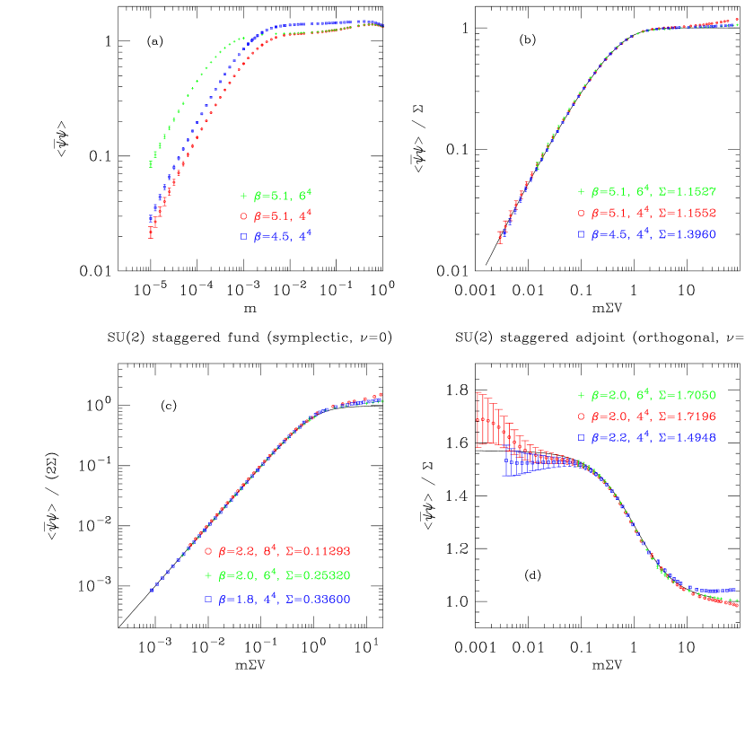
FIG. 1.: The condensate for staggered fermions in (a) the fundamental representation of SU(3) as function of the fermion mass, (b) rescaled form as a function of $\mu=m\Sigma V$, (c) the fundamental representation of SU(2), (d) the adjoint representation of SU(2).

II Staggered Fermions

Analytical predictions for the quenched chiral condensate and higher chiral susceptibilities are all restricted to sectors of fixed gauge field topology. As mentioned above, with staggered fermions lattice simulations of the chiral condensate at realistic values of the coupling do not see any trace of gauge field sectors except the one of topological charge $\nu=0$ [6]. The comparisons one can make are therefore slightly limited. On the other hand, computationally the staggered fermion formulation is extremely convenient for our purposes. We shall therefore start with a systematic study of the chiral condensate based on staggered fermions.

For the determination of the staggered quenched chiral condensate, we used a stochastic estimate method for several $\beta$ in SU(2) and SU(3) with fermions in the fundamental and adjoint representations. We are interested in solving the linear system of equations $D^{\dagger}(m)D(m)\eta(m)=\left(D^{\dagger}(0)D(0)+m^{2}\right)\eta(m)=b$ for some stochastic source $b$ and the staggered Dirac operator $D$. We can relate the solution $\eta(m)$ in a fixed background gauge field to the final quantities we are interested in with the following expressions:

$$\langle b|D^{-1}(m)|b\rangle = m\;b^{\dagger}\eta(m)$$ (16)

$$\langle b|(D^{\dagger}(m)D(m))^{-1}+D^{-2}(m)|b\rangle = 2\,m^{2}\;\eta^{\dagger}(m)\eta(m)$$ (17)

A multi-shift conjugate method [20] was used to solve the required linear system for several fermion masses. We supplemented these measurements with computations of the lowest 50 eigenvalues of the staggered Dirac operator, typically in 32 bit single precision. These eigenvalues were used to compute a truncated spectral sum approximation for the condensates at small fermion masses. The truncated spectral sum method greatly improved the statistics. However, for the small lattices ($4^{4}$ and $6^{4}$) typically on the order of 100000 configurations were needed. As will be discussed below, this reasonably large amount of statistics was necessary to adequately sample the lowest eigenvalue distribution of the Dirac operator probed by the small fermion masses used for our tests of the predictions of Chiral Random Matrix Theory. In addition, for the orthogonal ensemble cases, double precision was used for the eigenvalues.

FIG. 2.: The distribution of the lowest eigenvalue for staggered fermions in the adjoint representation of SU(2) at $\beta=2.0$ and $4^{4}$ corresponding to the orthogonal ensemble. The scale is greatly enlarged to show the leading edge of the distribution.

Consider first the gauge group SU(3) and staggered fermions in the fundamental representation. The universality class is thus that of the chUE, the same as in the continuum. In Fig. 1a we show the quenched chiral condensate as a function of the valence mass $m$ for a few different $\beta$-values, and various different lattice sizes. At the shown values of the lattice coupling $\beta$ the infinite-volume chiral condensate $\Sigma$ has already been determined to high accuracy from independent studies [10]. This means that the finite-size scaling function $\Sigma_{\nu}(\mu)$ of Eq. (4) is parameter-free. The first observation is that all the different data roughly collapse down on one universal scaling curve, once plotted against $\mu=m\Sigma V$ as in Fig. 1b. And the analytical prediction (4) for this curve is remarkably well reproduced by our lattice data. This of course just confirms on these lattice volumes and these $\beta$-values the observation first made by Verbaarschot [6] on the basis of data from the Columbia group. It is particularly interesting to look at the small-mass behavior. If we expand the condensate in (4) for small $\mu$, we get (for $\nu=0$)

$$\frac{\Sigma_{0}^{\rm{\mbox{c}hUE}}(\mu)}{\Sigma}=-\left(\ln(\frac{\mu}{2})+\gamma-\frac{1}{2}\right)\mu+{\cal O}(\mu^{3})~{},$$ (18)

where $\gamma$ is Euler’s constant. There is the expected term linear in $\mu$, but in addition a logarithmic correction of the form $\mu\ln(\mu)$. This latter term, which should not be confused with so-called “quenched chiral logarithms”, arises from the infrared part of the integral in Eq. (3), and is thus very sensitive to the fall-off of $\rho_{s}(\zeta)$ near $\zeta\sim 0$. Indeed, for the chUE the quenched microscopic spectral density reads [3]:

$$\rho_{s}^{(0)}(\zeta)=\frac{\zeta}{2}\left[J_{0}(\zeta)^{2}+J_{1}(\zeta)^{2}\right]~{},$$ (19)

which for small values of $\zeta$ behaves like $\rho_{s}^{(0)}(\zeta)=\zeta/2-\zeta^{3}/8+\ldots$. The leading linear term here is responsible for the $\mu\ln(\mu)$ piece in (18). The chUE cases with $\nu\geq 1$ lend themselves more easily to an analysis of the low-mass behavior of the condensate, since the integrals

$$\int_{0}^{\infty}d\zeta\frac{\rho_{s}^{(\nu)}(\zeta)}{\zeta^{2}}$$

in those cases are convergent. We can thus make the following rewriting:

$$\frac{\Sigma_{\nu}(\mu)}{\Sigma}~{}~{}=~{}~{}2\mu\int_{0}^{\infty}\!d\zeta\frac{\rho_{s}^{(\nu)}(\zeta)}{\zeta^{2}+\mu^{2}}~{}~{}+~{}~{}\frac{\nu}{\mu}~{}~{}=~{}~{}2\mu\int_{0}^{\infty}\!d\zeta~{}\rho_{s}^{(\nu)}(\zeta)\left[\frac{1}{\zeta^{2}}-\frac{\mu^{2}}{\zeta^{2}(\zeta^{2}+\mu^{2})}\right]~{}~{}+~{}~{}\frac{\nu}{\mu}~{},$$ (20)

and consider each term separately. It follows that the leading, linear, term in the expansion of $\Sigma_{\nu}(\mu)$ for $\nu\geq 1$ has as coefficient the first Leutwyler-Smilga sum rule (as extended to this quenched case) [1, 5]:

$$\frac{\Sigma_{\nu}^{\rm{\mbox{c}hUE}}(\mu)}{\Sigma}~{}=~{}\frac{\nu}{\mu}~{}+~{}2\mu\left\langle\sum_{n>0}\frac{1}{\zeta_{n}^{2}}\right\rangle_{\nu}+\ldots~{}=~{}\frac{\nu}{\mu}~{}+~{}\frac{1}{2\nu}\mu+\ldots\ldots$$ (21)

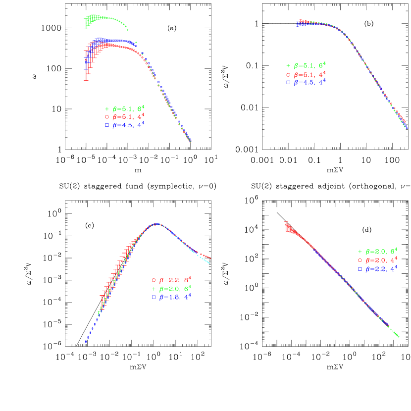
FIG. 3.: The quenched susceptibility $\omega$ for staggered fermions in (a) the fundamental representation of SU(3) as function of the fermion mass, (b) in rescaled form as a function of $\mu=m\Sigma V$, (c) the fundamental representation of SU(2), (d) the adjoint representation of SU(2).

We next turn to gauge group SU(2) and staggered fermions in the fundamental representation. The analytical prediction is here that of the chSE universality class, with a chiral condensate as in Eqs. (7) and (9). We again choose $\beta$-values for which the infinite-volume chiral condensate $\Sigma$ is known to high accuracy, so that the analytical predictions (7) and (9) also are parameter-free. One remark is in order here: in the chSE universality class every eigenvalue is doubly degenerate. The analytical predictions from RMT consider only one of the eigenvalues from each degenerate pair. A stochastic estimate of the condensate, on the other hand, contains the contribution from both eigenvalues of each pair, and is thus a factor two larger. We have therefore divided the stochastic estimate of the condensate by this factor two in order to compare to the analytical prediction. In Fig. 1c we show how all data nicely collapse down on the universal scaling function (7) for $N_{f}=0$. The agreement is seen to be extraordinarily good over more than three orders of magnitude.

The microscopic spectral density of that case [9] reads as follows for $N_{f}=0$:

$$\rho_{s}^{(0)}(\zeta)=\zeta J_{1}(2\zeta)^{2}-\frac{\pi\zeta}{2}\left({\mbox{\bf H}}_{0}(2\zeta)J_{0}(2\zeta)J_{1}(2\zeta)-{\mbox{\bf H}}_{1}(2\zeta)J_{0}(2\zeta)^{2}\right)~{},$$ (22)

where ${\mbox{\bf H}}_{n}(x)$ is the $n$th order Struve function. Since the small-$\zeta$ expansion is of the form $\rho_{s}^{(0)}(\zeta)=\zeta^{3}/3+\ldots$, we can make the same rewriting as above (see Eq. (20)) and consider each term separately. It follows that also here the leading, linear, term in the expansion of $\Sigma_{0}(\mu)$ has as coefficient the first Leutwyler-Smilga sum rule for that case [1, 5]:

$$\frac{\Sigma_{0}^{\rm{\mbox{c}hSE}}(\mu)}{\Sigma}~{}=~{}2\mu\left\langle\sum_{n>0}\frac{1}{\zeta_{n}^{2}}\right\rangle_{0}+\ldots~{}=~{}\mu+\ldots$$ (23)

This linear behavior with coefficient one is precisely what is observed in Fig. 1c. The same argument goes through also for sectors of non-trivial winding numbers $\nu$ , in which case the formula reads:

$$\frac{\Sigma_{\nu}^{\rm{\mbox{c}hSE}}(\mu)}{\Sigma}~{}=~{}\frac{\nu}{\mu}+2\mu\left\langle\sum_{n>0}\frac{1}{\zeta_{n}^{2}}\right\rangle_{\nu}+\ldots~{}=~{}\frac{\nu}{\mu}+\frac{1}{1+2|\nu|}\mu+\ldots\ldots$$ (24)

We finally present lattice gauge theory data for the SU(2) gauge group, and staggered fermions in the adjoint representation. Here data should align on the universal scaling curve of the chOE universality class (see Eq. (15)), and we show the results of a few high statistics (but rather small) lattice volumes and two different $\beta$-values in Fig. 1d. The $\beta$-values were again chosen on the basis of having already a good estimate for the infinite-volume chiral condensate $\Sigma$ (for the adjoint representation) [11]. The analytical curve is seen to have a surprising behavior: it rises, even here in the $\nu=0$ case, with decreasing (rescaled) fermion mass $\mu$. This unusual feature is a reflection of a peculiarity of the quenched microscopic spectral density $\rho_{s}^{(0)}(\zeta)$ for the chOE (see the third of ref. [3] and $e.g.$ [19]),

$$\rho_{s}^{(0)}(\zeta) = \frac{\zeta}{2}J_{1}(\zeta)^{2}+\frac{1}{2}J_{0}(\zeta)\left[1-\frac{1}{2}\pi\zeta\left({\mbox{\bf H}}_{0}(\zeta)J_{1}(\zeta)-{\mbox{\bf H}}_{1}(\zeta)J_{0}(\zeta)\right)\right]~{}.$$ (25)

Contrary to all other microscopic spectral densities for the chiral ensembles, the above function does not vanish at $\zeta=0$. This is an artifact of the quenched limit, and it implies that in this quenched theory one can have spontaneous symmetry breaking even if one is taking the limit $V\to\infty$ and $m\to 0$ in a correlated manner. Conventionally the possibility of spontaneous symmetry breaking implies that one first sends the volume $V$ to infinity, and only subsequently takes the massless limit, $m\to 0$:

$$\Sigma~{}\equiv~{}\lim_{m\to 0}\lim_{V\to\infty}\langle\bar{\psi}\psi\rangle~{}.$$ (26)

In the quenched case corresponding to the chOE we observe that spontaneous symmetry breaking can occur even if we take the simultaneous limit $V\to\infty$ and $m\to 0$, with $mV$ fixed. This holds only in the $\nu=0$ sector. For $\nu\neq 0$ we face the usual situation that the chiral condensate diverges like $1/\mu$. This holds in the quenched theory as well when we sum over topological charges [18].

Also in this case we can analyze the limit of $\mu\to 0$ analytically for $\nu=0$. The reason for the unusual phenomenon of a constant mass-dependent chiral condensate in the limit $\mu\to 0$ is the term $J_{0}(\zeta)/2$ in Eq. (25). It is this term that leads to a non-vanishing microscopic spectral density at $\zeta=0$, and one can easily confirm that it is also this term that is responsible for the leading small-$\mu$ behavior of the chiral condensate in this case. Using

$$\int_{0}^{\infty}\!d\zeta\frac{J_{0}(\zeta)}{\zeta^{2}+\mu^{2}}~{}=~{}\frac{\pi}{2\mu}(I_{0}(\mu)-{\mbox{\bf L}}_{0}(\mu))$$ (27)

and the small-$\mu$ expansion of the modified Struve function ${\mbox{\bf L}}_{0}(\mu)=2\mu/\pi+\ldots$, we see that only the first piece contributes in the limit $\mu\to 0$. From Eqs. (3) and (25) we finally get.

$$\frac{\Sigma_{0}^{\rm{\mbox{c}hOE}}(\mu)}{\Sigma}~{}=~{}\frac{\pi}{2}+~{}{\cal O}(\mu)$$ (28)

for this universality class. An approach towards this constant value is seen in the data of Fig. 1d, but the signal obviously gets rather noisy around $\mu\sim 10^{-3}$ for these lattice volumes. We show in Fig. 2 magnified plot of the distribution of the smallest eigenvalue along with the curve for the fit for the $4^{4}$ lattice. We see there is a reasonable sampling of the distribution for the very small eigenvalues, but even larger statistics beyond our 135000 configurations are needed to really adequately sample this region and hence give very reliable estimates for the condensate. Again we see that the chiral condensate is an extremely sensitive probe of the smallest Dirac eigenvalue spectrum. For example, the statistical fluctuation that causes a small surplus of eigenvalues very close to the origin in Fig. 2 reflects itself directly in the slightly larger chiral condensate in Fig. 1d. The deviation is seen clearly on the non-logarithmic vertical scale.

In sectors of non-vanishing topological charge $\nu$, the microscopic spectral density vanishes at the origin, and if it were not for the $\nu/\mu$-piece, the mass-dependent chiral condensate would then also vanish as $\mu\to 0$, even in the infinite-volume limit. For example, for $\nu=1$ the expansion for small $\mu$ reads in this case

$$\frac{\Sigma_{1}^{\rm{\mbox{c}hOE}}(\mu)}{\Sigma}~{}=~{}\frac{1}{\mu}-\frac{1}{2}\left(\ln(\frac{\mu}{2})+\gamma-1\right)\mu+{\cal O}(\mu^{3})~{},$$ (29)

with, again, a $\mu\ln(\mu)$-term in addition to the purely linear contribution.

Other physical observables can of course be extracted from the finite-volume partition function. We shall here focus on one such observable, a chiral susceptibility $\omega(\mu)$ which we define as:

$$\frac{\omega_{\nu}(\mu)}{\Sigma^{2}V}~{}\equiv~{}4\mu^{2}\int_{0}^{\infty}\!d\zeta\frac{\rho_{s}^{(\nu)}(\zeta;\mu)}{(\zeta^{2}+\mu^{2})^{2}}+\frac{2\nu}{\mu^{2}}~{}.$$ (30)

We expect this quantity to be a more sensitive probe of the rescaled eigenvalues $\zeta$ at a specific rescaled mass $\mu$ than the chiral condensate because of the higher power occurring in the denominator of the integrand. This quantity is especially easy to compute in the quenched limit, where the spectral density is $\mu$-independent. One then has

$$\frac{\omega_{\nu}(\mu)}{\Sigma^{2}V} = -2\mu\frac{\partial}{\partial\mu}\left[\int_{0}^{\infty}d\zeta\frac{\rho_{s}^{(\nu)}(\zeta)}{(\zeta^{2}+\mu^{2})}+\frac{\nu}{2\mu^{2}}\right]$$ (31)

$$= -\mu\frac{\partial}{\partial\mu}\left.\left[\frac{\Sigma_{\nu}(\mu)}{\mu}\right]\right/\Sigma$$ (32)

$$= \left.\left[\frac{\Sigma_{\nu}(\mu)}{\mu}-\Sigma^{\prime}_{\nu}(\mu)\right]\right/\Sigma~{}.$$ (33)

That combination is particularly useful in testing the small deviation from linear behavior of $\Sigma_{\nu}(\mu)$ in, for instance, the case corresponding to the chUE with $\nu=0$. In general, for a quenched condensate of the form

$$\frac{\Sigma_{\nu}(\mu)}{\Sigma}~{}=~{}\frac{\nu}{\mu}+A\mu+B\mu\ln(\mu)+C\mu^{2}+\ldots$$ (34)

we indeed find

$$\frac{\omega_{\nu}(\mu)}{\Sigma^{2}V}~{}=~{}\frac{2\nu}{\mu^{2}}-B-C\mu+\ldots~{}.$$ (35)

The linear term in $\Sigma_{\nu}(\mu)$ has cancelled, and the asymptotic behavior for $\mu\to 0$ gives us the constant in front of the $\mu\ln(\mu)$-term in $\Sigma_{\nu}(\mu)$.

For the chUE universality class, the quenched susceptibility defined above becomes quite simple:

$$\frac{\omega_{\nu}^{\rm{\mbox{c}hUE}}(\mu)}{\Sigma^{2}V}~{}=~{}2I_{\nu+1}(\mu)K_{\nu-1}(\mu)+\frac{2\nu}{\mu^{2}}$$ (36)

which has the small $\mu$ expansion

$$\frac{{\omega_{\nu}^{\rm{\mbox{c}hUE}}(\mu)}}{\Sigma^{2}V}~{}=~{}\frac{2\nu}{\mu^{2}}~{}+~{}\cases{1+\frac{1}{2}(\ln(\frac{\mu}{2})+\gamma-\frac{1}{4})\mu^{2}+{\cal O}(\mu^{4})&if $\nu=0$\cr-\frac{1}{4}(\ln(\frac{\mu}{2})+\gamma)\mu^{2}+{\cal O}(\mu^{4})&if $\nu=1$\cr\frac{1}{4\nu(\nu^{2}-1)}\mu^{2}+{\cal O}(\mu^{4})&if $\nu\geq 2$\cr}$$ (37)

Of course, similar expressions can be derived for the partially quenched cases.

In Fig. 3a we show raw data for $\omega$ for the same lattice couplings and lattice volumes as in Fig. 1. Again, these raw data beautifully collapse down on the one single scaling function $\omega_{0}(\mu)$ when rescaled according to the above prescription, as shown in Fig. 3b. We emphasize again that the data for $\omega(\mu)$ are much more sensitive probes of the microscopic spectral density of the Dirac operator than the chiral condensate itself.

For the chSE and chOE universality classes the general expressions for $\omega(\mu)$ are quite involved, but the cases with $\nu=0$ and $1$ become relatively simple. The prediction for the chSE universality class in a sector of topological charge zero and one reads:

$$\frac{\omega_{0}^{\rm{\mbox{c}hSE}}(\mu)}{\Sigma^{2}V}~{}=~{}\pi\left[K_{0}(2\mu)+2\mu K_{1}(2\mu)\right]\left[{\mbox{\bf L}}_{0}(2\mu)I_{1}(2\mu)-{\mbox{\bf L}}_{1}(2\mu)I_{0}(2\mu)\right]-4\mu K_{1}(2\mu)I_{2}(2\mu)~{},$$ (38)

$$\frac{\omega_{1}^{\rm{\mbox{c}hSE}}(\mu)}{\Sigma^{2}V} = \frac{2}{\mu^{2}}+4K_{1}(2\mu)\left[I_{3}(2\mu)+\mu I_{2}(2\mu)\right]+8K_{2}(2\mu)I_{2}(2\mu)$$ (40)

$$-\pi\left[3K_{2}(2\mu)+2\mu K_{1}(2\mu)\right]\left[{\mbox{\bf L}}_{0}(2\mu)I_{1}(2\mu)-{\mbox{\bf L}}_{1}(2\mu)I_{0}(2\mu)\right]$$

with the small $\mu$ expansion

$$\frac{\omega_{\nu}^{\rm{\mbox{c}hSE}}(\mu)}{\Sigma^{2}V}~{}=~{}\frac{2\nu}{\mu^{2}}~{}+~{}\cases{-\frac{4}{3}(\ln(\mu)+\gamma-\frac{1}{4})\mu^{2}+{\cal O}(\mu^{4})&if $\nu=0$\cr\frac{1}{15}\mu^{2}+{\cal O}(\mu^{4})&if $\nu=1$.\cr}$$ (41)

The analogous prediction for the chOE case is

$$\frac{\omega_{0}^{\rm{\mbox{c}hOE}}(\mu)}{\Sigma^{2}V} = \frac{\pi}{2}\left[K_{0}(\mu)+\mu K_{1}(\mu)\right]\left[{\mbox{\bf L}}_{0}(\mu)I_{1}(\mu)-{\mbox{\bf L}}_{1}(\mu)I_{0}(\mu)\right]-\mu K_{1}(\mu)I_{2}(\mu)$$ (43)

$$+\frac{\pi}{2\mu}\left[I_{0}(\mu)-{\mbox{\bf L}}_{0}(\mu)\right]-\frac{\pi}{2}\left[I_{1}(\mu)-{\mbox{\bf L}}_{1}(\mu)\right]+1~{},$$

$$\frac{\omega_{1}^{\rm{\mbox{c}hOE}}(\mu)}{\Sigma^{2}V}~{}=~{}\frac{2}{\mu^{2}}+K_{0}(\mu)I_{2}(\mu)+K_{1}(\mu)I_{1}(\mu)$$ (44)

with the small $\mu$ expansions

$$\frac{\omega_{\nu}^{\rm{\mbox{c}hOE}}(\mu)}{\Sigma^{2}V}~{}=~{}\frac{2\nu}{\mu^{2}}~{}+~{}\cases{\frac{\pi}{2\mu}-\frac{\pi}{8}\mu-\frac{1}{6}(\ln(\frac{\mu}{2})+\gamma-\frac{19}{12})\mu^{2}+{\cal O}(\mu^{3})&if $\nu=0$\cr\frac{1}{2}+\frac{1}{8}(\ln(\frac{\mu}{2})+\gamma-\frac{1}{2})\mu^{2}+{\cal O}(\mu^{4})&if $\nu=1$.\cr}$$ (45)

We show the rescaled data for gauge group SU(2) and staggered fermions in the fundamental representation in Fig. 3c, and compare these rescaled data with the analytical prediction (38). The agreement is quite good, except for the very smallest lattice volume ($4^{4}$ at $\beta=1.8$). Finally, in Fig. 3d we show analogous data for gauge group SU(2) and staggered fermions in the adjoint representation, where the analytical prediction (of the chOE universality class) is as given in Eq. (43). Again the agreement is perfect.

From the Leutwyler-Smilga sum rules and from the small mass expansions for the chiral condensate we can make a general prediction for the agreement of the condensate with the RMT predictions based on how well the microscopic spectral density fits the corresponding RMT predictions. We see in the unitary case that the coefficient of the linear order in the mass prediction for the sum rule Eq. (21) is dependent on all the non-zero eigenvalues (appropriately weighted) in the spectral sum for $\nu>0$. For the $\nu=0$ case, we find the condensate will depend most strongly on the leading edge of the lowest eigenvalue for very small $\mu$. This dependence is related to the appearance of the $\mu\ln(\mu)$ term in Eq. (18). For the symplectic case, the coefficient in Eq. (24) is predicted for all $\nu\geq 0$ (no appearance of a $\ln(\mu)$ term at leading order). For the orthogonal case, there is no sum-rule and we can expect a strong dependence on the smallest non-zero eigenvalue in all topologies at small fermion mass. In general then if the microscopic spectral density agrees well for many oscillations with RMT we can expect reasonable agreement for the condensates with RMT in the ensembles and topological sectors where the sum-rules apply. In the other cases, when probing with a small fermion mass there can be a strong dependence on how well the smallest eigenvalue is sampled.

At the same time, there is another competing effect that can make the non-zero topology data fit reasonably well with the RMT predictions. From the solution to $\eta(m)$ in Eq. (17), we see that when $m\rightarrow 0$ the cutoff for the bottom spectrum of $D^{\dagger}(0)D(0)$ is the smallest eigenvalue which will be non-zero. Hence, $\eta$ goes to a constant at $m=0$. However, $\langle\bar{\psi}\psi\rangle$ and $\omega$ go down with an explicit $m$ or $m^{2}$ factor. The RMT predictions are non-trivial because, in the unitary case for example, a $\mu\ln(\mu)$ term is generated. At higher topology, the $\ln(\mu)$ term moves to higher ${\cal O}(\mu)$. Hence, we can see trivial agreement with RMT at higher Q when we probe the smallest eigenvalue. However, we still have to get the overall infinite volume scale $\Sigma$ correct and that is non-trivial.

III Topology: Overlap Fermions

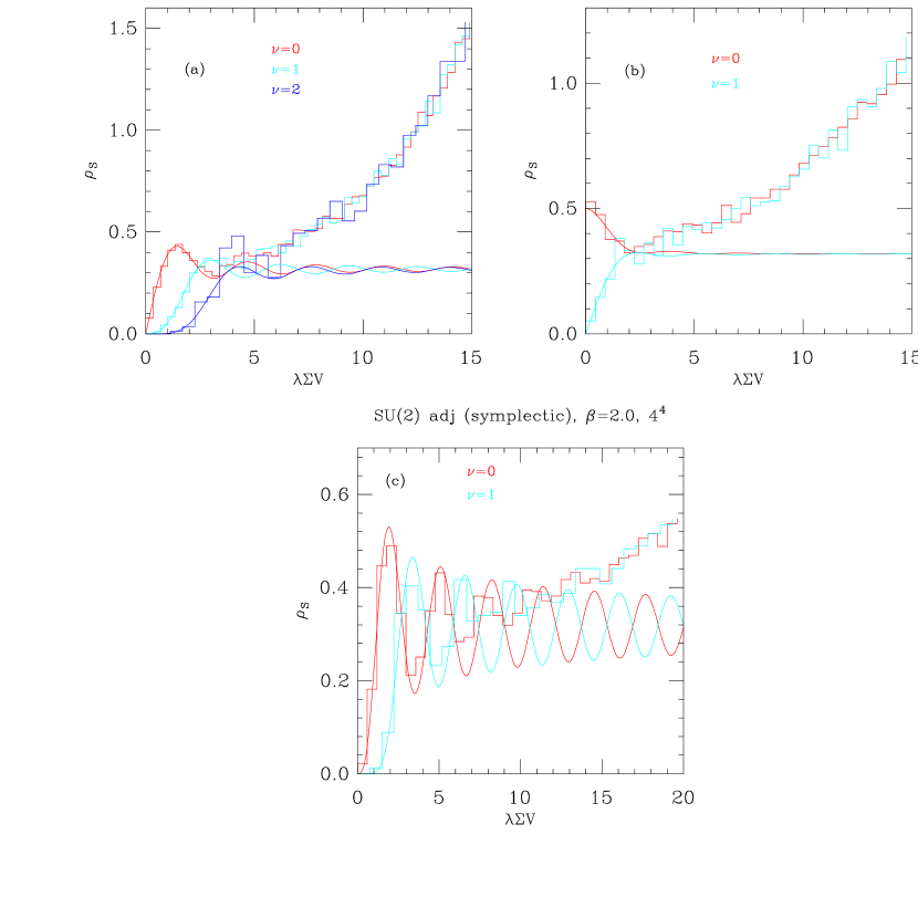
FIG. 4.: The microscopic spectral density for overlap fermions in (a) the fundamental representation of SU(3) (unitary), (b) the fundamental representation of SU(2) (orthogonal), (c) the adjoint representation of SU(2) (symplectic). Deviations from the analytical predictions (smooth curves) beyond a few oscillations are due to the rather small physical volumes considered.

It is particularly interesting to test the analytical predictions for sectors with non-trivial topological charge. While staggered fermions are unsuitable for this, there now exist lattice-fermion formulations which correctly reproduce those chiral Ward identities that are sensitive to gauge field topology. Because they share the same Ward identities as continuum fermions, their effective Lagrangians coincide with those of conventional chiral perturbation theory. In particular, in the scaling limit (1), these lattice fermions will give rise to the same Leutwyler-Smilga effective Lagrangians (depending on the gauge groups and color representations), and will hence fall into exactly the same universality classes as continuum fermions.

The overlap Dirac operator [15] derived from the overlap formalism [21] is a proper realization of a single flavor massless fermion on the lattice that separates lattice gauge fields into different topological classes based on the number of exact fermion zero modes. The massive overlap Dirac operator is given by

$$D(m)~{}=~{}\frac{1}{2}\left[1+m+(1-m)\gamma_{5}\epsilon(H_{w})\right]~{}.$$ (46)

with $0\leq m\leq 1$ describing fermions with positive mass all the way from zero to infinity and where $H_{w}$ is the hermitian Wilson-Dirac operator with a negative Wilson-Dirac mass on the lattice [15, 16, 22]. Here $\epsilon(x)$ indicates the sign function.

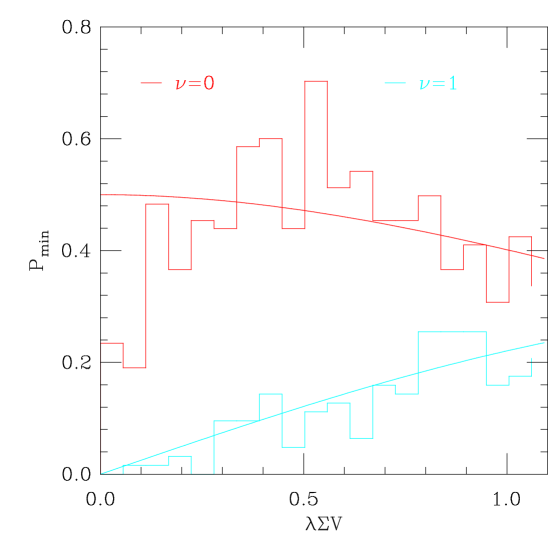
FIG. 5.: The distribution of the lowest eigenvalue for overlap fermions in the orthogonal ensemble. The scale is enlarged to show the leading edge of the distribution.

The external fermion propagator is given by

$${\tilde{D}}^{-1}(m)=(1-m)^{-1}\left[D^{-1}(m)-1\right]~{}.$$ (47)

The subtraction at $m=0$ is evident from the original overlap formalism [21] and the massless propagator anti-commutes with $\gamma_{5}$ [15]. With our choice of subtraction and overall normalization the propagator satisfies the relation

$$m\langle b|\Bigl{[}\gamma_{5}{\tilde{D}}^{-1}(m)\Bigr{]}^{2}|b\rangle=\langle b|{\tilde{D}}^{-1}(m)|b\rangle\ \ \ \ \forall\ \ b\ \ \ {\rm satisfying}\ \ \ \gamma_{5}|b\rangle=\pm|b\rangle$$ (48)

for all values of $m$ in an arbitrary gauge field background [16]. If chiral symmetry is broken, the right hand side of Eq. (48) is non-zero in the massless limit implying that the pion mass goes to zero as the square root of the fermion mass. Since $(\gamma_{5}D(m))^{2}$ commutes with $\gamma_{5}$, its eigenvectors are chiral. In the basis where $(\gamma_{5}D(m))^{2}$ is diagonal, $\gamma_{5}D(m)$ is block diagonal with each block being a $2\times 2$ matrix [16]. Exact zero eigenvalues of $(\gamma_{5}D(m))^{2}$ are paired with unit eigenvalues of $(\gamma_{5}D(m))^{2}$ with the opposite chirality. These eigenvectors of $(\gamma_{5}D(m))^{2}$ are also eigenvectors of $D(m)$ and therefore the topological zero modes of $D(m)$ are chiral. We shall denote the non-zero eigenvalues of $(\gamma_{5}D(m))^{2}$ by $\lambda_{i}^{2}$ with $0<\lambda_{i}^{2}<1$. In terms of these eigenvalues, the chiral condensate and chiral susceptibility in a fixed gauge field background are given by [16]

$$\frac{1}{V}\sum_{x}\langle\bar{\psi}(x)\psi(x)\rangle_{A}=\frac{1}{V}{\rm Tr}[{\tilde{D}}^{-1}]=\frac{|\nu|}{mV}+\frac{1}{V}\sum_{i}\frac{2m(1-\lambda_{i}^{2})}{\lambda_{i}^{2}(1-m^{2})+m^{2}}~{}.$$ (49)

and

$$\omega={1\over m}\langle\bar{\psi}\psi\rangle_{A}-{d\over dm}\langle\bar{\psi}\psi\rangle_{A}={1\over V}\left({\rm Tr}(\gamma_{5}\tilde{D})^{-2}(m)+{\rm Tr}\tilde{D}^{-2}(m)\right)~{}.$$ (50)

Similar to Eq. (48), we have [23]

$$\langle b|{\tilde{D}}^{-1}(m)|b\rangle = {m\over 1-m^{2}}b^{\dagger}\left(\eta(m)-b\right)$$ (51)

$$\langle b|(\gamma_{5}\tilde{D})^{-2}(m)+\tilde{D}^{-2}(m)|b\rangle = {2m^{2}\over(1-m^{2})^{2}}\left(\eta^{\dagger}(m)-b^{\dagger}\right)\left(\eta(m)-b\right)$$ (52)

where

$$H_{o}^{2}(m)\eta(m)=b\qquad{\rm with}\qquad H_{o}(m)=\gamma_{5}D(m),\quad\gamma_{5}b=\pm b\quad.$$ (53)

We note that

$$H_{o}^{2}(m)=D^{\dagger}(m)D(m)=D(m)D^{\dagger}(m)=\left(1-m^{2}\right)\left[H_{o}^{2}(0)+{m^{2}\over 1-m^{2}}\right]$$ (54)

with

$$H_{o}^{2}(0)\chi_{\pm}=\left[{1\over 2}+{1\over 4}\left(\gamma_{5}\pm 1)\right)\epsilon(H_{w})\right]\chi_{\pm}\qquad{\rm with}\quad\gamma_{5}\chi_{\pm}=\pm\chi_{\pm}\quad.$$ (55)

Eq. (54) implies that we can solve the set of equations $H_{o}^{2}(m)\eta(m)=b$ for several masses, $m$, simultaneously (for the same right hand $b$) using the multiple Krylov space solver described in Ref. [20]. In our tests we used fermion masses from $0$ to $0.999$. However, for comparisons to RMT we only consider the fermion mass range from $m=10^{-4}$ up to $0.999$.

The first term on the right hand side of Eq. (49) is due to the presence of $|\nu|$ exact zero modes in a fixed gauge field background. By working in the chiral sector where $(\gamma_{5}D(m))^{2}$ has no zero modes, it is possible to compute the second term in Eq. (49) and investigate the onset of chiral symmetry breaking on the lattice [16]. Note that the relation (49) is an exact identity at any lattice spacing. It is of the same form as Eq. (3), up to terms vanishing with the ultraviolet cut-off. The bare fermion mass enters the overlap Dirac operator in a non-trivial way and is proportional to the mass parameter $m$ in (46) only for small $m$, i.e. only up to terms of relative ${\cal O}(a^{2})$. The proportionality factor, $Z_{m}$, depends in particular on the mass in the Wilson-Dirac operator used [16]. Since $Z_{m}$ is the inverse of the wave function renormalization constant [16], the rescaled mass parameter $\mu=m\Sigma V$ is independent of these $Z$-factors and agrees with the continuum definition up to terms vanishing with the ultraviolet cut-off.

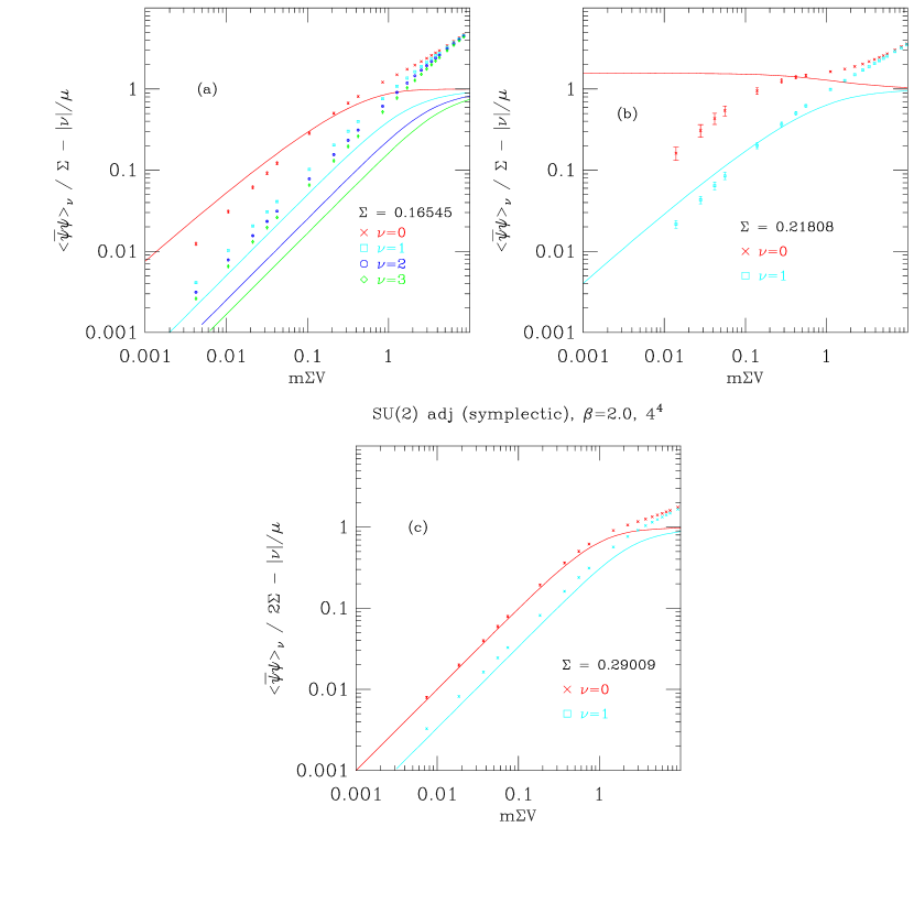
FIG. 6.: The rescaled condensate for overlap fermions in (a) the fundamental representation of SU(3) as function of $\mu=m\Sigma V$, (b) the fundamental representation of SU(2), (c) the adjoint representation of SU(2).

The infinite-volume chiral condensate $\Sigma$ differs significantly, at the same $\beta$-values, from that of staggered fermions. However, in the cases we shall present here this one single parameter $\Sigma$ has already been extracted to high precision from the distribution of the smallest Dirac operator eigenvalue [13]. The analytical predictions for $\Sigma_{\nu}(\mu)$ are thus parameter-free also in these cases.

On all the gauge configurations used for the measurement of the condensate a few low lying eigenvalues have previously been determined [13]. We thus know the number and chirality of all zero modes, and hence the topological charge. As mentioned already, when zero modes are present, we perform the stochastic estimate in the sector with opposite chirality. In topologically trivial gauge fields, we perform the stochastic estimate in the positive chirality sector.

We are now ready to test some of the predictions for overlap fermions in the finite-volume regime. The first observation is that the universality classes of continuum fermions coincide with those of overlap fermions. We begin by comparing the microscopic spectral density $\rho_{s}(\zeta)$ with the predictions of RMT. In Fig. 4 are the results for different topological sectors for all the ensembles. The curves are the predictions using the infinite volume $\Sigma$ previously determined [13]. We see good agreement for the first oscillation (essentially the lowest eigenvalue contribution) for all topological sectors and the best agreement in the symplectic case in Fig. 4c. However, the data rapidly deviates up from the curve for higher eigenvalues. This is a finite-volume effect since as the volume increases the scale of the eigenvalues decreases into the region where RMT applies. The infinite volume chiral condensate $\Sigma$ sets the scale for the eigenvalues, and since the condensate is larger for staggered fermions compared to overlap fermions at corresponding parameters, the eigenvalues for staggered fermions occur closer to zero where there is a corresponding better agreement for more oscillations with the RMT predictions.

Nevertheless, we can expect to find the best agreement of $\omega_{\nu}$ with the RMT predictions where the fermion mass is probing the scale of eigenvalues in $\rho_{s}(\zeta)$ that are in best agreement. For the chiral condensate $\langle\bar{\psi}\psi\rangle_{\nu}$ the agreement with RMT will depend on the overall $\rho_{s}(\zeta)$ which we remarked is best for the symplectic case. Since the spectral density does not match the RMT prediction for many oscillations in the unitary case as seen in Fig. 4a, we expect higher topologies to not be well described by RMT.

In addition, we can expect problems for comparisons of observables for small fermions masses when the $\rho_{s}(z)$ has not been adequately sampled, and this problem is most pronounced in the orthogonal case. Compared to the staggered fermion example in Fig. 2, we do not have enough statistics and large enough volumes to adequately sample the leading edge of the eigenvalue distributions shown in detail in Fig. 5.

We continue with tests of the predictions for $\Sigma_{\nu}(\mu)$ in the chUE case, using quenched overlap fermions and gauge group SU(3). Shown in Fig. 6a are some data for gauge field sectors with $\nu=0\ldots 3$. We stress that for the sectors of non-vanishing $\nu$ we have subtracted the somewhat trivial $\nu/\mu$ term, which otherwise would completely dominate the plot. What is shown is thus not the chiral condensate per se, but rather $\Sigma_{\nu}(\mu)/\Sigma-|\nu|/\mu$. The agreement in the $\nu=0$ sector is good, but while the data for the $\nu=1$, 2, and 3 qualitatively display the right behavior, they are nevertheless somewhat off the analytical predictions.

In Fig. 7a we show the subtracted $\omega_{\nu}/\Sigma^{2}V$ for the unitary case. As mentioned before, this observable is a more sensitive probe of the eigenvalue distribution at a fixed fermion mass and should yield better agreement when the corresponding $\rho_{s}(\zeta)$ is in good agreement with the RMT predictions. We see good agreement for $z=m\Sigma V>0.05$ in all topology sectors, but below this value there are deviations related to the lack of small eigenvalues in $\rho_{s}$ and the small volume. For the orthogonal ensemble we find even worse agreement for $\Sigma_{\nu}(\mu)/\Sigma-|\nu|/\mu$ shown in Fig. 6b, but find a small mass region ($0.4\mathrel{\hbox to0.0pt{\lower 3.0pt\hbox{$\mathchar 536\relax$}\hss}\raise 2.0pt\hbox{$\mathchar 316\relax$}}z\mathrel{\hbox to0.0pt{\lower 3.0pt\hbox{$\mathchar 536\relax$}\hss}\raise 2.0pt\hbox{$\mathchar 316\relax$}}4$) in $\omega_{\nu}/\Sigma^{2}V$ shown in Fig. 7b where we simultaneously have an adequately sampled distribution of very small eigenvalues and good agreement of $\rho_{s}(z)$ with RMT.

We next turn to gauge group SU(2) and overlap fermions in the adjoint representation where we find the expected good agreement with analytical predictions for the $\nu=0$ and $1$ sectors (we found almost no configurations in the sectors of higher topological charge in this case). These graphs are shown in Fig. 6c and Fig. 7c.

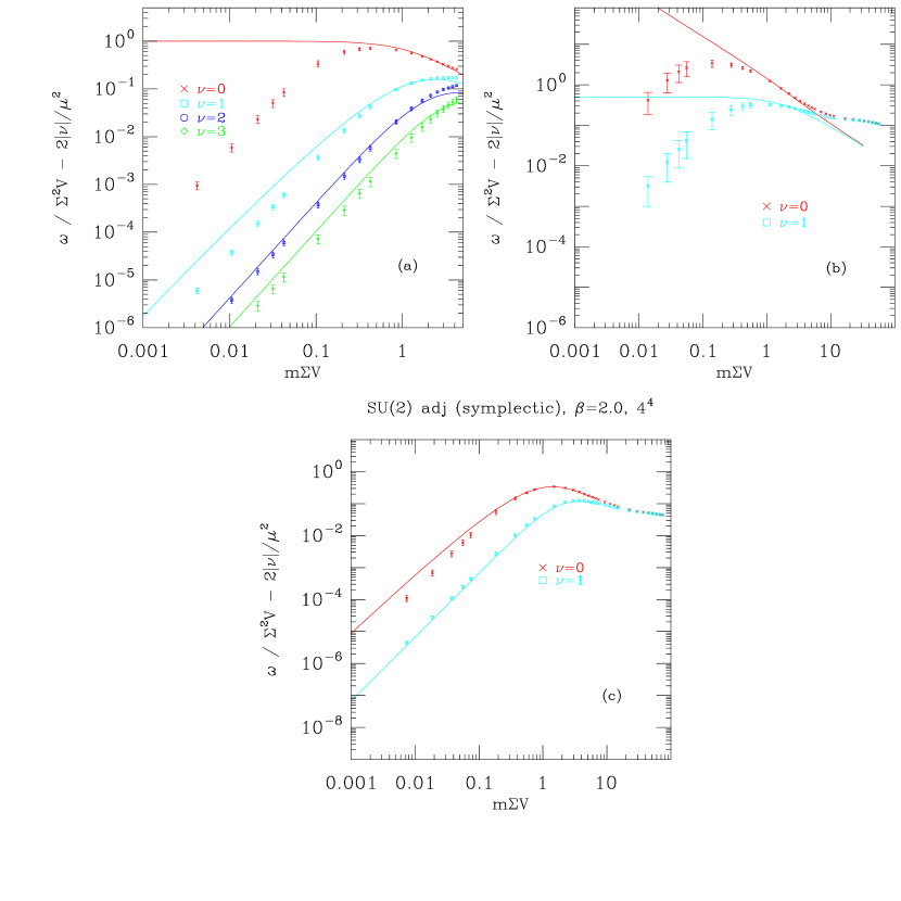
FIG. 7.: The rescaled quenched susceptibility $\omega$ for overlap fermions in (a) the fundamental representation of SU(3) as a function of $\mu=m\Sigma V$. (b) the fundamental representation of SU(2), (c) in the adjoint representation of SU(2).

IV Conclusions

We have performed a systematic series of Monte Carlo tests of the analytical predictions for the chiral condensate and related chiral susceptibilities in the finite-volume scaling region of Eq. (1). In four dimensions there are three universality classes with which to compare, conveniently classified in Random Matrix Theory terminology by means of chiral versions of the three classical matrix ensembles, $i.e.$, chSE, chUE and chOE. Once the infinite-volume chiral condensate $\Sigma$ is known, there are parameter-free finite-volume scaling functions with which to compare data. As we have shown, results for all three universality classes with topological charge $\nu=0$ are nicely reproduced by staggered fermions. To test the analytical predictions for gauge field sectors of non-trivial topological winding numbers, we have also considered overlap fermions, which possess exact zero modes in topologically non-trivial gauge fields. Here there is qualitatively good agreement, with even excellent agreement in the case of the chSE universality class. The deviations from the RMT predictions observed in the other cases are understood to be due to either finite volume effects or the relatively modest statistics we were able to obtain in the simulations with overlap fermions.

The results presented here clearly show the power of the finite-size analysis that has come out of the study of finite-volume effective partition functions and Random Matrix Theory. In contrast to conventional finite-size scaling analysis near critical points, we are here in the unusual situation of knowing not only the right scaling variables, but also parameter-free exact analytical predictions for the scaling quantities. In this particular corner of those non-Abelian or Abelian gauge theories that support spontaneous breaking of chiral symmetry the exact analytical predictions have thus very clearly been confirmed by direct numerical studies.

Acknowledgments: The work of P.H.D. has been partially supported by EU TMR grant no. ERBFMRXCT97-0122, and the work of R.G.E. and U.M.H. has been supported in part by DOE contracts DE-FG05-85ER250000 and DE-FG05-96ER40979. In addition, P.H.D. and U.M.H. acknowledge the financial support of NATO Science Collaborative Research Grant no. CRG 971487. This work was completed at the Aspen Center for Physics, and we thank the center for the excellent working conditions provided to us.

REFERENCES

-
[1]
J. Gasser and H. Leutwyler, Phys. Lett. 188B, 477 (1987).
H. Leutwyler and A. Smilga, Phys. Rev. D46, 5607 (1992). - [2] E.V. Shuryak and J.J.M. Verbaarschot, Nucl. Phys. A560, 306 (1993).
-
[3]
J.J.M. Verbaarschot and I. Zahed, Phys. Rev. Lett. 70,
3852 (1993).
J.J.M. Verbaarschot, Phys. Lett. B329, 351 (1994); Nucl. Phys. B426, 559 (1994). -
[4]
G. Akemann, P.H. Damgaard, U. Magnea and S. Nishigaki,
Nucl. Phys. B487, 721 (1997).
P.H. Damgaard and S.M. Nishigaki, Nucl. Phys. B518, 495 (1998).
M.K. Şener and J.J.M. Verbaarschot, Phys. Rev. Lett. 81, 248 (1998). -
[5]
J.J.M. Verbaarschot, Phys. Rev. Lett. 72, 2531 (1994).
A. Smilga and J.J.M. Verbaarschot, Phys. Rev D51, 829 (1995).
M.A. Halasz and J.J.M. Verbaarschot, Phys. Rev D52, 2563 (1995). - [6] J.J.M. Verbaarschot, Phys. Lett. B368, 137 (1996).
-
[7]
P.H. Damgaard, Phys. Lett. B424, 322 (1998).
G. Akemann and P.H. Damgaard, Nucl. Phys. B519, 682 (1998); Phys. Lett. B432, 390 (1998).
S.M. Nishigaki, P.H. Damgaard and T. Wettig, Phys. Rev. D58, 087704 (1998). -
[8]
J.C. Osborn, D. Toublan and J.J.M. Verbaarschot, Nucl. Phys.
B540, 317 (1998).
P.H. Damgaard, J.C. Osborn, D. Toublan and J.J.M. Verbaarschot, Nucl. Phys. B547, 305 (1999).
D. Toublan and J.J.M. Verbaarschot, hep-th/9904199. -
[9]
M.E. Berbenni-Bitsch, S. Meyer, A. Schäfer,
J.J.M. Verbaarschot and T. Wettig, Phys. Rev. Lett. 80, 1146 (1998).
M.E. Berbenni-Bitsch, S. Meyer, T. Wettig, Phys. Rev. D58, 071502 (1998).
J.-Z. Ma, T. Guhr and T. Wettig, Eur. Phys. J. A2, 87 (1998).
M.E. Berbenni-Bitsch et al., Phys. Lett. B438, 14 (1998); hep-lat/9901013. -
[10]
P.H. Damgaard, U.M. Heller and A. Krasnitz, Phys. Lett.
B445, 366 (1999).
M. Göckeler, H. Hehl, P.E.L. Rakow, A. Schäfer and T. Wettig, Phys. Rev. D59, 094503 (1999). - [11] R.G. Edwards, U.M. Heller and R. Narayanan, hep-lat/9902021.
- [12] F. Farchioni, I. Hip, C.B. Lang and M. Wohlgenannt, Nucl. Phys. B549, 364 (1999).
- [13] R.G. Edwards, U.M Heller, J. Kiskis and R. Narayanan, Phys. Rev. Lett. 82, 4188 (1999).
- [14] S.Chandrasekharan, Nucl. Phys. B (Proc. Suppl) 42, 475 (1995).
- [15] H. Neuberger, Phys. Lett. B417, 141 (1998); hep-lat/9808036; hep-lat/9807009.
- [16] R.G. Edwards, U.M. Heller and R. Narayanan, Phys. Rev. D59, (1999) 094510.
- [17] P.H. Damgaard, Phys. Lett. B425, 151 (1998).
- [18] P.H. Damgaard, hep-th/9807026, hep-th/9903096.
-
[19]
H. Widom, solv-int/9804005.
P.J. Forrester, T. Nagao and G. Honner, cond-mat/9811142. - [20] A. Frommer, S. Güsken, T. Lippert, B. Nöckel, K. Schilling, Int. J. Mod. Phys. C6, 627 (1995); B. Jegerlehner, hep-lat/9612014.
- [21] R. Narayanan and H. Neuberger, Nucl. Phys. B B443 (1995) 305.
- [22] R.G. Edwards, U.M. Heller and R. Narayanan, Nucl. Phys. B540, 457 (1999).
- [23] R.G. Edwards, U.M. Heller and R. Narayanan, hep-lat/9905028, to be published in a special issue of Parallel Computing.