Random Matrix Theory, Chiral Perturbation Theory, and Lattice Data

Abstract

Recently, the chiral logarithms predicted by quenched chiral perturbation theory have been extracted from lattice calculations of hadron masses. We argue that the deviations of lattice results from random matrix theory starting around the so-called Thouless energy can be understood in terms of chiral perturbation theory as well. Comparison of lattice data with chiral perturbation theory formulae allows us to compute the pion decay constant. We present results from a calculation for quenched SU(2) with Kogut–Susskind fermions at $\beta=2.0$ and $2.2$.

PACS: 11.30.Rd; 11.15.Ha; 12.38.Gc; 05.45.Pq
Keywords: chiral perturbation theory; random matrix theory; lattice gauge calculations; SU(2) gauge theory

, , , , , , and

For many observables, quenched chiral perturbation theory predicts contributions which are logarithmic in the quark mass [1, 2]. Their identification in lattice gauge results is a long standing problem. It seems that the latest numerical results [3, 4, 5, 6] on hadron masses in quenched lattice simulations allow for an approximate determination of these $\ln(m)$ contributions. (For an earlier attempt see [7].) The determination of these logarithms is an important test of chiral perturbation theory (chPT) which in turn plays a central role for the connection of low-energy hadron theory on one side and perturbative and lattice QCD on the other.

In a completely independent development, it has been shown by several authors that chiral random matrix theory (chRMT) is able to reproduce quantitatively microscopic spectral properties of the Dirac operator obtained from QCD lattice data (see the reviews [8, 9] and Refs. [10, 11, 12, 13]). Moreover, the limit up to which the microscopic spectral correlations can be described by random matrix theory (the analogue of the Thouless energy of statistical physics) was analyzed theoretically in [14, 15] and identified for quenched SU(2) (SU(3)) lattice calculations in [16] ([17]). It has also been shown [18] that the results obtained in chRMT can be derived directly from field theory, providing a firm theoretical basis for the RMT approach.

In this letter we want to study the Dirac spectrum beyond the Thouless energy using chPT (for a first investigation of this issue see [19]). Lattice Monte Carlo calculations inevitably involve a finite volume, so we have to consider chPT in a finite volume, too. Chiral RMT should be valid for masses $m$ up to the Thouless energy $\sim 1/L^{2}$ ($L$ = linear extent of the lattice), whereas the chPT formulae are supposed to work if $m$ is larger than a certain lower limit scaling like $1/L^{4}$. Thus we expect a domain of common applicability for sufficiently large lattices. The data we are going to analyze were obtained for the gauge group SU(2) in the quenched approximation with staggered fermions. They consist of complete spectra of the lattice Dirac operator. As the bare coupling in these data is relatively strong, we shall set up our (quenched) chPT in such a way that only those symmetries are taken into account which are exactly realized on the lattice. We will find that this eliminates terms $\propto\ln(m)$ from the quenched chiral condensate, which are present if one starts from the continuum symmetries.

In the following we shall use the chiral condensate and the scalar susceptibilities, so we first give their definitions. For a finite lattice and a non-vanishing valence-quark mass, the chiral condensate is given by

$$\sigma_{\mathrm{lattice}}(m)=\frac{1}{N}\left\langle\sum_{k=1}^{N}\frac{1}{{\mathrm{i}}\lambda_{k}+m}\right\rangle\;.$$ (1)

In the quenched theory, the connected susceptibility is given simply by

$$\chi^{\mathrm{conn}}_{\mathrm{lattice}}(m)=\frac{\partial}{\partial m}\sigma(m)=-\frac{1}{N}\left\langle\sum_{k=1}^{N}\frac{1}{({\mathrm{i}}\lambda_{k}+m)^{2}}\right\rangle\;.$$ (2)

The disconnected susceptibility is defined on the lattice by

$$\chi^{\mathrm{disc}}_{\mathrm{lattice}}=\frac{1}{N}\left\langle\sum_{k,l=1}^{N}\frac{1}{({\mathrm{i}}\lambda_{k}+m)({\mathrm{i}}\lambda_{l}+m)}\right\rangle-\frac{1}{N}\left\langle\sum_{k=1}^{N}\frac{1}{{\mathrm{i}}\lambda_{k}+m}\right\rangle^{2}\;.$$ (3)

Here, $N=L^{4}$ denotes the number of lattice points, and the $\lambda_{k}$ are the Dirac eigenvalues. Note that each of the doubly degenerate eigenvalues (for gauge group SU(2)) counts only once.

With the abbreviation $F(x)=\int^{1}_{0}\!\d t\>I_{0}(tx)$ the chRMT result for the chiral condensate reads

$$\frac{\sigma_{\mathrm{RMT}}}{\Sigma}=2u\Bigl{[}I_{0}(2u)K_{0}(2u)+I_{1}(2u)K_{1}(2u)-K_{0}(2u)F(2u)\Bigr{]}\,,$$ (4)

where $\Sigma$ denotes the absolute value of the chiral condensate for infinite volume and vanishing mass, and the rescaled mass parameter $u$ is given by $u=m\Sigma L^{4}$. The functions $I_{\nu}$, $K_{\nu}$ are modified Bessel functions. For the connected susceptibility chRMT predicts

$$\frac{\chi^{\mathrm{conn}}_{\mathrm{RMT}}}{N\Sigma^{2}}=2K_{1}(2u)\Bigl{[}2uF(2u)-I_{1}(2u)\Bigr{]}\,.$$ (5)

The chRMT result for the disconnected susceptibility is slightly more complicated [16], but can be simplified to read:

$$\frac{\chi^{\mathrm{disc}}_{\mathrm{RMT}}}{N\Sigma^{2}} = 1-K_{0}(2u)I_{0}(2u)+\Bigl{[}K_{0}(2u)-2uK_{1}(2u)\Bigr{]}F(2u)$$ (6)

$${}-\biggl{\{}2uK_{0}(2u)F(2u)-2u\Bigl{[}K_{0}(2u)I_{0}(2u)+K_{1}(2u)I_{1}(2u)\Bigr{]}\biggr{\}}^{2}\;.$$

In Ref. [16] it was demonstrated for $\chi^{\mathrm{disc}}$ that chRMT describes the Monte Carlo data perfectly up to values of $m$ which scale like $1/L^{2}$ (the analogue of the Thouless energy). This is also true for $\sigma$ and $\chi^{\mathrm{conn}}$.

We want to understand the behavior of the data beyond the Thouless energy using (quenched) chPT. Chiral perturbation theory uses effective actions for the Goldstone bosons to describe the mass and volume dependence of, e.g., the chiral condensate and the susceptibilities. The effective action depends only on the symmetries and the corresponding breaking pattern. The predictions of chRMT are equivalent [18] to the leading-order results from the so-called $\epsilon$-expansion in chPT, where $m=O(\epsilon^{4})$ and $1/L=O(\epsilon)$. The coefficients in this expansion are nontrivial functions of $u=m\Sigma L^{4}$. On the other hand, standard chiral perturbation theory (the so-called $p$-expansion) sets $m=O(p^{2})$, $1/L=O(p)$ and expands in powers of $p$ (see, e.g., [20]).

Applying chPT in the present context we have to deal with two technical problems. Since the data that we want to analyze are taken in the quenched approximation we ought to work with the quenched version of chiral perturbation theory. Secondly, we work at rather strong coupling where we cannot expect the continuum symmetries to be already effectively restored. So we should consider only symmetries which are exact on the lattice (and the corresponding Goldstone bosons), a situation usually not dealt with in the literature.

Below the Thouless energy the first problem becomes trivial when we use the chRMT results, because these depend explicitly on the number of flavors which we can set equal to zero. Furthermore they also depend on the topological charge $\nu$ (i.e. the number of zero modes of the Dirac operator), which suggests a solution to the second problem: At strong coupling, the Dirac operator of staggered fermions has no exact topological zero modes due to lattice artifacts, hence the lattice results should be compared with the case $\nu=0$ [12]. Indeed, one finds very good agreement.

Above the Thouless energy, in the regime of the $p$-expansion, we should use (partially) quenched chPT taking into account the pattern according to which chiral symmetry is spontaneously broken in the case of staggered fermions with gauge group SU(2). To the best of our knowledge, an analysis of this particular case has not been done before. In the following, we present our own, somewhat unorthodox, approach to this problem in order to avoid the intricacies of quenched chiral perturbation theory.

Starting point is a partition function of the form:

$$\begin{array}[]{l}\displaystyle Z(m_{v},m_{s},L)\\ \displaystyle\propto\exp\left[VT(m_{v},m_{s})-\frac{1}{2}\sum_{Q}\left\{K_{Q}\sum_{p}\ln\left({\hat{p}}^{2}+m_{Q}^{2}(m_{v},m_{s})\right)\right\}\right].\end{array}$$ (7)

$T(m_{v},m_{s})$ is the classical (or saddle-point) contribution to the free energy, which we will assume is a smooth function of the quark masses, and independent of lattice volume. The double sum represents the 1-loop contribution coming from light composite bosons. The sum runs over the allowed momenta $p$ ($p_{\mu}=2\pi n_{\mu}/L$ with integer $n_{\mu}$) and over particle type $Q$. $K_{Q}$ is the multiplicity of the particles of type $Q$. On the lattice we will use the expression

$${\hat{p}}^{2}\equiv 2\sum_{\mu}(1-\cos p_{\mu})$$ (8)

for the boson kinetic term, where $p_{\mu}$ is expressed in lattice units.

We have introduced two quark masses, valence quarks with mass $m_{v}$, and sea quarks with mass $m_{s}$. We have $N_{v}$ ‘generations’ of the quarks with mass $m_{v}$, and $N_{s}$ generations of the quarks with mass $m_{s}$. In the continuum limit, each staggered ‘generation’ yields four fermion flavors. We will take the limit $N_{v}\rightarrow 0$, so that the valence quarks are quenched.

To use Eq. (7) we need the masses and multiplicities of all the light bosons. For mesons made of two different quark flavors ${\bar{q}}_{i}q_{j}$ we use the expression

$$m^{2}=A(m_{i}+m_{j})/2.$$ (9)

This applies to $(N_{s}+N_{v})(N_{s}+N_{v}-1)$ bound states.

For the remaining $N_{s}+N_{v}$ ‘flavor-diagonal’ mesons we should also consider annihilation (see Fig. 1).

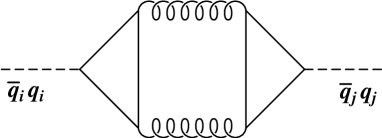
Figure 1: Annihilation diagram for pseudoscalar mesons.

However, with staggered fermions there is an anomaly-free U(1) symmetry, which would cause the amplitude for ${\bar{q}}_{i}q_{i}\rightarrow{\bar{q}}_{j}q_{j}$ to vanish if either $m_{i}=0$ or $m_{j}=0$. Therefore we expect the annihilation amplitude to be proportional to $m_{i}m_{j}$ for small quark masses. In the final formulae this leads to contributions which possess only a mild $m$–dependence (there is at least one more power of $m$ than in the leading contribution). Hence these are hard to distinguish from the smooth background and cannot be fitted reliably. To leading order, it is consistent to neglect the annihilation terms, and we end up with $N_{v}$ ($N_{s}$) states with $m^{2}=Am_{v}$ ($m^{2}=Am_{s}$) in the ‘flavor-diagonal’ sector. (Note that for the gauge group SU(3) there are special cases where the annihilation terms contribute to leading order and can therefore not be neglected.)

For the SU(2) gauge group the symmetry when all quarks are massless is $\mathrm{U}(2N_{v}+2N_{s})$, which spontaneously breaks to $\mathrm{O}(2N_{v}+2N_{s})$ [21]. This is further broken to $\mathrm{O}(2N_{v})\times\mathrm{O}(2N_{s})$ if the valence and sea quarks are given different bare masses. The extra symmetry present when the gauge group is SU(2) transforms mesons into baryons ($q_{i}q_{j}$ and ${\bar{q}_{i}}{\bar{q}_{j}}$ states), which thus have the same mass as the mesons. These states will have mass-squared given by the same formula as the different-flavor mesons, i.e., $m^{2}=A(m_{i}+m_{j})/2$. Therefore we have to include more light bosons in our partition function leading to the spectrum given in Table 1.

Table 1: The light particle spectrum for gauge group SU(2).

$m^{2}$	multiplicity
$Am_{v}$	$2N_{v}^{2}+N_{v}$
$Am_{s}$	$2N_{s}^{2}+N_{s}$
$A(m_{v}+m_{s})/2$	$4N_{v}N_{s}$

In SU(2) we just sum over the non-degenerate eigenvalues (according to the RMT conventions), so our definition of the chiral condensate $\sigma$ is

$$\sigma(m_{v},m_{s},L)=\lim_{N_{v}\rightarrow 0}\left(\,\frac{1}{V}\frac{1}{2N_{v}}\,\frac{1}{Z}\,\frac{\partial Z}{\partial m_{v}}\right)\,.$$ (10)

If we substitute the multiplicities of Table 1 into Eq. (7) we get

$$\sigma(m_{v},m_{s},L) = S+C_{c}m_{v}+C_{d}2N_{s}m_{s}-\frac{A}{4L^{4}}\sum_{p}\frac{1}{{\hat{p}}^{2}+Am_{v}}$$ (11)

$${}-\frac{AN_{s}}{L^{4}}\sum_{p}\frac{1}{2{\hat{p}}^{2}+A(m_{v}+m_{s})}\,,$$

where the first three terms parametrize the classical background contribution. Differentiating $\sigma$ to give the susceptibilities we find for identical valence and sea quark masses, $m_{v}=m_{s}=m$,

$$\chi^{\mathrm{conn}}(m,m,L) = C_{c}+\frac{A^{2}(1+N_{s})}{4L^{4}}\sum_{p}\frac{1}{({\hat{p}}^{2}+Am)^{2}}\,,$$ (12)

$$\chi^{\mathrm{disc}}(m,m,L) = C_{d}+\frac{A^{2}}{8L^{4}}\sum_{p}\frac{1}{({\hat{p}}^{2}+Am)^{2}}\,.$$ (13)

Sending finally also $N_{s}$ to zero we arrive at formulae appropriate for comparison with our quenched Monte Carlo data. Note that the leading behavior of these chPT formulae for $m\to 0$ coincides with the leading term for $m\to\infty$ of the chRMT formulae. This is in accordance with the existence of a mass range where both theories apply.

In the thermodynamic limit we obtain from (11), (12), and (13) chiral logarithms:

$$\sigma(m) = \left(S-\frac{1}{4}Aa_{0}\right)-\frac{A^{2}}{64\pi^{2}}m\ln(Am)+\left(C_{c}-\frac{1}{4}A^{2}a_{1}\right)m$$ (14)

$${}+\frac{A^{3}}{512\pi^{2}}m^{2}\ln(Am)-\frac{1}{4}A^{3}a_{2}m^{2}+\cdots\,,$$

$$\chi^{\mathrm{conn}}(m) = -\frac{A^{2}}{64\pi^{2}}\ln(Am)+\left(C_{c}-\frac{1}{4}A^{2}a_{1}-\frac{A^{2}}{64\pi^{2}}\right)$$ (15)

$${}+\frac{A^{3}}{256\pi^{2}}m\ln(Am)+A^{3}\left(\frac{1}{512\pi^{2}}-\frac{1}{2}a_{2}\right)m+\cdots\,,$$

$$\chi^{\mathrm{disc}}(m) = -\frac{A^{2}}{128\pi^{2}}\ln(Am)+\left(C_{d}-\frac{1}{8}A^{2}a_{1}-\frac{A^{2}}{128\pi^{2}}\right)$$ (16)

$${}+\frac{A^{3}}{512\pi^{2}}m\ln(Am)+A^{3}\left(\frac{1}{1024\pi^{2}}-\frac{1}{4}a_{2}\right)m+\cdots$$

for $N_{s}=0$ and $m_{v}=m_{s}=m$. The numerical constants $a_{0}$, $a_{1}$, and $a_{2}$ take the values $a_{0}=0.1549$, $a_{1}=-0.03035$, $a_{2}=0.002776$.

To highlight the special properties of the SU(2) gauge group with staggered fermions, we will now compare with the conventional continuum calculation with gauge group SU(3). In this case there are no light ‘Goldstone baryons’, so we only need to consider meson states. The other important difference is that in the continuum the chiral U(1) has an anomaly. This means that the annihilation term in the meson mass matrix does not need to vanish in the chiral limit. This leads us to the following ansatz for the mass-squared matrix, $M^{c}$, for the flavor-diagonal mesons:

$$M^{c}=A\,\mathrm{diag}\left(m_{v},\ldots,m_{v},m_{s},\ldots,m_{s}\right)+m_{0}^{2}\left(\matrix{1&\ldots&1\cr\vdots&\ddots&\vdots\cr 1&\ldots&1}\right)$$ (17)

with $N_{v}$ ($N_{s}$) entries $Am_{v}$ ($Am_{s}$) on the diagonal of the first part. Here $m_{0}$ is a constant with the dimensions of mass, which does not vanish in the chiral limit.

Besides $N_{v}-1$ eigenvalues equal to $Am_{v}$ and $N_{s}-1$ eigenvalues equal to $Am_{s}$ this mass matrix has two non-trivial eigenvalues. The important thing to note is that one of them does not vanish in the chiral limit but goes to the value $(N_{v}+N_{s})m_{0}^{2}$. This is the state corresponding to the continuum $\eta^{\prime}$.

Using the continuum multiplicities and masses in our formula for $Z$ and omitting the smooth background for simplicity leads to

$$\sigma^{c}(m,m,L)=\frac{A}{2L^{4}}\sum_{p}\frac{m_{0}^{2}(1-N_{s}^{2})-N_{s}({\hat{p}}^{2}+Am)}{({\hat{p}}^{2}+Am)({\hat{p}}^{2}+N_{s}m_{0}^{2}+Am)}$$ (18)

(the case of equal valence and sea quark masses is sufficient to illustrate the main differences between staggered and continuum fermions). For $N_{s}\neq 0$ the $L\rightarrow\infty$ limit of this $\sigma$ is

$$\sigma^{c}(m,m,\infty) = \frac{A}{2N_{s}}\frac{Am}{16\pi^{2}}\ln\left[\frac{Am}{N_{s}m_{0}^{2}+Am}\right]$$ (19)

$${}-\,\frac{AN_{s}}{2}\left(a_{0}+\frac{Am}{16\pi^{2}}\ln(Am)+a_{1}Am\right)$$

$${}-\,\frac{A}{2}\left(\frac{m_{0}^{2}}{16\pi^{2}}\ln(N_{s}m_{0}^{2}+Am)+a_{1}m_{0}^{2}\right)+\cdots\,.$$

At small $m$ the most severe singularity is of the form $m\ln m$.

However in the quenched limit the behaviour is different. Then Eq. (18) reduces to

$$\sigma^{c}(m,m,L)=\frac{A}{2L^{4}}\sum_{p}\frac{m_{0}^{2}}{({\hat{p}}^{2}+Am)^{2}}\,,$$ (20)

which is more singular at small $m$. The thermodynamic limit of this expression is

$$\sigma^{c}(m,m,\infty)=\frac{Am_{0}^{2}}{2}\left[-\frac{1}{16\pi^{2}}\left(\ln(Am)+1\right)-a_{1}+\cdots\right]\,.$$ (21)

Now we have a more severe singularity ($\propto\ln m$) in the small mass limit. This is the well-known quenched chiral logarithm. We do not get this logarithm in our regime because the relevant U(1) symmetry is not anomalous.

Figure 2: Connected and disconnected susceptibility for selected values of $L$ and $\beta$. The chRMT results are shown as dotted lines, the chPT fits are displayed as full curves. Data points within the fit range are marked by circles, else by crosses. For clarity the statistical errors of the data points are not shown, in most cases they are smaller than the symbols.

We have confronted our chPT formulae with lattice Monte Carlo data. We used staggered fermions in the quenched approximation and two values of the coupling strength $\beta$, $\beta=2.0$ and $\beta=2.2$. The lattice sizes and numbers of configurations are given in Table 2. The chPT formulae are able to describe the deviations from the RMT results beyond the Thouless energy very well. Examples of joint fits of $\chi^{\mathrm{conn}}$ and $\chi^{\mathrm{disc}}$ with (12) and (13), respectively, are presented in Fig. 2. It seems that for the connected susceptibility our lattices are not large enough to exhibit clearly a domain where both chRMT and chPT (to the order considered) are applicable, although there is a trend towards the formation of such a window with increasing $L$.

Joint fits of $\chi^{\mathrm{conn}}$ and $\chi^{\mathrm{disc}}$ lead to the values for $A$ given in Table 2. The error has been estimated from the variation of the results under changes of the fit interval. This is a somewhat subjective procedure of determining the error and goes beyond the purely statistical contribution. However we consider it to be more realistic than using the MINUIT errors. The smaller errors on the larger lattices thus reflect the increasing reliability of our numbers.

Due to the Gell-Mann–Oakes–Renner relation the parameter $A$ is related to the chiral condensate $\Sigma$ (for infinite volume and vanishing mass) and the pion decay constant $f_{\pi}$ by

$$A=\frac{2\Sigma}{f_{\pi}^{2}}\;.$$ (22)

The chiral condensate $\Sigma$ can be determined independently, e.g. from the mean value of the smallest eigenvalue according to the RMT formula [12]

$$\Sigma=\frac{2.06636\cdots}{L^{4}\langle\lambda_{\mathrm{min}}\rangle}\;.$$ (23)

The corresponding numbers together with the resulting values for $f_{\pi}$ are also given in Table 2. Note that except for the smallest lattices the results are nearly independent of $L$ demonstrating the reliability of our procedure.

Table 2: Simulation parameters together with fit results for the chPT parameter $A$ and the chiral condensate $\Sigma$. The value of the pion decay constant $f_{\pi}$ following from the Gell-Mann–Oakes–Renner relation is given in the last column.

$\beta$	$L$	configs	$A$	$\Sigma$	$f_{\pi}$
2.0	4	49978	13.5(9)	0.1157(2)	0.131(4)
	6	24976	11.6(2)	0.1258(3)	0.147(1)
	8	14290	10.9(1)	0.1253(4)	0.1516(7)
	10	4404	10.4(1)	0.1239(7)	0.1544(9)
2.2	6	22288	14.5(5)	0.0540(2)	0.086(2)
	8	13975	13.8(2)	0.0568(2)	0.0907(7)
	10	2950	13.6(1)	0.0573(4)	0.0918(5)
	12	1382	13.4(1)	0.0576(6)	0.0927(6)

In conclusion, we have verified predictions of chiral random matrix theory and (quenched) chiral perturbation theory by means of lattice Monte Carlo data. In particular, we have investigated finite-volume effects and found a domain of common validity of both theories. It was crucial to base the analysis on the lattice symmetries and not on the continuum symmetries. We were also able to determine the pion decay constant. The extension of the present analysis to the case of gauge group SU(3) will be the subject of an upcoming publication.

References

- [1] C.W. Bernard and M.F.L. Golterman, Phys. Rev. D46 (1992) 853; Nucl. Phys. B (Proc. Suppl.) 34 (1994) 331; Phys. Rev. D49 (1994) 486; M.F.L. Golterman, Acta Phys. Polon. B25 (1994) 1731.
- [2] J.N. Labrenz and S.R. Sharpe, Nucl. Phys. B (Proc. Suppl.) 34 (1994) 335; Phys. Rev. D54 (1996) 4595.
- [3] W. Bardeen, A. Duncan, E. Eichten and H.B. Thacker, Nucl. Phys. B (Proc. Suppl.) 73 (1999) 243.
- [4] M. Göckeler, R. Horsley, V. Linke, D. Pleiter, P.E.L. Rakow, G. Schierholz, A. Schiller, P. Stephenson and H. Stüben, Nucl. Phys. B (Proc. Suppl.) 73 (1999) 237.
- [5] R. Burkhalter, Nucl. Phys. B (Proc. Suppl.) 73 (1999) 3.
- [6] R.D. Kenway, Nucl. Phys. B (Proc. Suppl.) 73 (1999) 16.
- [7] S. Kim and D.K. Sinclair, Phys. Rev. D52 (1995) 2614.
- [8] For a recent review on random matrix theory in general, see T. Guhr, A. Müller-Groeling, H.A. Weidenmüller, Phys. Rept. 299 (1998) 189.
- [9] For a review on RMT and Dirac spectra, see the recent review by J.J.M. Verbaarschot, hep-ph/9902394, and references therein.
- [10] J.J.M. Verbaarschot, Phys. Lett. B 368 (1996) 137.
- [11] M.A. Halasz and J.J.M. Verbaarschot, Phys. Rev. Lett. 74 (1995) 3920.
- [12] M.E. Berbenni-Bitsch, S. Meyer, A. Schäfer, J.J.M. Verbaarschot and T. Wettig, Phys. Rev. Lett. 80 (1998) 1146.
- [13] J.-Z. Ma, T. Guhr and T. Wettig, Eur. Phys. J. A 2 (1998) 87, 425.
- [14] R.A. Janik, M.A. Nowak, G. Papp and I. Zahed, Phys. Rev. Lett. 81 (1998) 264.
- [15] J.C. Osborn and J.J.M. Verbaarschot, Phys. Rev. Lett. 81 (1998) 268; Nucl. Phys. B525 (1998) 738.
- [16] M.E. Berbenni-Bitsch, M. Göckeler, T. Guhr, A.D. Jackson, J.-Z. Ma, S. Meyer, A. Schäfer, H.A. Weidenmüller, T. Wettig and T. Wilke, Phys. Lett. B 438 (1998) 14.
- [17] M. Göckeler, H. Hehl, P.E.L. Rakow, A. Schäfer and T. Wettig, Phys. Rev. D59 (1999) 094503.
- [18] J.C. Osborn, D. Toublan and J.J.M. Verbaarschot, Nucl. Phys. B540 (1999) 317; P.H. Damgaard, J.C. Osborn, D. Toublan and J.J.M. Verbaarschot, Nucl. Phys. B547 (1999) 305.
- [19] M.E. Berbenni-Bitsch, M. Göckeler, H. Hehl, S. Meyer, P.E.L. Rakow, A. Schäfer and T. Wettig, hep-lat/9901013.
- [20] J. Gasser and H. Leutwyler, Phys. Lett. B 188 (1987) 477.
- [21] H. Kluberg-Stern, A. Morel and B. Petersson, Nucl. Phys. B215 (1983) 527.