Abstract

SU($N_{c}$) Yang-Mills theory is investigated at finite densities of $N_{f}$ heavy quark flavors. The calculation of the (continuum) quark determinant in the large-mass limit is performed by analytic methods and results in an effective gluonic action. This action is then subject to a lattice representation of the gluon fields and computer simulations. The approach maintains the same number of quark degrees of freedom as in the continuum formulation and a physical heavy quark limit (to be contrasted with the quenched approximation $N_{f}\rightarrow 0$). The proper scaling towards the continuum limit is manifest. We study the partition function for given values of the chemical potential as well as the partition function which is projected onto a definite baryon number. First numerical results for an SU(2) gauge theory are presented. We briefly discuss the breaking of the color-electric string at finite densities and shed light onto the origin of the overlap problem inherent in the Glasgow approach.

 

PACS: 11.15.Ha, 12.38.Gc

1 Introduction

The next generation of particle accelerators (RHIC, LHC), which will start operating at the beginning of the next millennium, will probe the deconfined regime of QCD, the theory of strong interactions, and might reveal exotic states of hadronic matter which appear under extreme conditions, i.e., temperature and density. Due to a significant increase in computational power in the recent past, numerical simulations of lattice QCD have provided insights into the high temperature and zero density phase and have predicted a series of interesting phenomena [1], such as deconfinement and restoration of chiral symmetry. Unfortunately, an adequate description of finite density hadron matter is still lacking due to conceptual problems in setting up an appropriate ”statistical” measure which can be handled in computer simulations.

The generic approach to Yang-Mills thermodynamics at finite densities is based on the introduction of a non-zero chemical potential. In the case of a SU(2) gauge group, the fermion determinant is real and can be included in the probabilistic measure. Numerical simulations can be performed by using standard algorithms [2], although this numerical approach consumes a lot of computer time due to the non-local nature of the action. Recent progress for the case of a SU(2) gauge group can be found in [3]. In the case of a SU(3) gauge group, the fermion determinant acquires imaginary parts for a non-vanishing chemical potential and cannot be considered to be part of the probabilistic measure. The most prominent example to circumvent this conceptual difficulty is the so-called Glasgow algorithm [4]. There, the fermion determinant is considered to be part of the correlation function to be calculated, and the probabilistic measure of zero-density Yang-Mills theory is used to generate the gauge field configurations. However, it turns out that this approach suffers from the so-called ”overlap” problem implying that for realistic lattice sizes an unrealistic number of Monte-Carlo steps is necessary to achieve reliable results [5].

In order to alleviate this problem, the so-called quenched approximation, i.e., the limit $N_{f}\rightarrow 0$, where $N_{f}$ is the number of quark flavors, greatly reduces the numerical task for practical calculations. While in the case of real QCD one expects a drastic change in the hadron density for a chemical potential $\mu=\mu_{onset}\approx m_{B}/3$ ($m_{B}$ is the baryon mass), the onset value $\mu_{onset}$ which is extracted from quenched lattice QCD seems to be unnaturally small [6]. Subsequently, it turned out that the quenched approximation, i.e., the limit $N_{f}\rightarrow 0$, of lattice QCD does not meet with the naive expectation that this limit coincides with the heavy quark limit of real QCD [7].

The confining properties of Yang-Mills theory in the desired limit where the quark mass and the chemical potential are simultaneously made large (heavy quark limit) while the density of quarks is kept finite and non-zero were first investigated in [8, 9]. Using Kogut-Susskind quarks, this limit simplifies the fermion determinant and allows a significant improvement of the statistics [9]. A recent breakthrough [10] was achieved by resorting to the heavy quark limit in addition to the use of the canonical ensemble, i.e., the hadron system of fixed density (by contrast to the grand-canonical ensemble of fixed chemical potential). The canonical approach involves the grand-canonical partition function with imaginary values of the chemical potential as first pointed out in [11]. A great simplification arises in this case from the fact that the fermion determinant is real. The numerical analysis of [10] reveals that the deconfinement phase transition becomes a cross-over at finite density (see also [9]). The string between static quark breaks yielding a constant heavy quark potential at large distances.

In this paper, we present a new approach to Yang-Mills theory at a finite density of heavy quarks. We shall calculate the continuum fermion determinant for arbitrary entries for the gluon field in the large mass limit (rather than in the quenched approximation $N_{f}\rightarrow 0$) using the Schwinger proper-time regularization. The result is a gauge invariant action of the gluon fields, depending on an UV-regulator $\Lambda$, and is added to the standard action of Yang-Mills theory. The total result can be discretized on a lattice with lattice spacing $a$ by standard methods and can be used as input for computer simulations. In the critical limit $\Lambda\rightarrow\infty$, $a\rightarrow 0$, physical quantities become independent of the regularization scheme, and the results for observables are independent of the choice of the technique, i.e., lattice regularization or Schwinger proper-time regularization of the fermion determinant. The advantages of our approach are as follows: firstly, the starting point of the calculation is the continuum quark determinant with the correct number of degrees of freedom. The approach is not plagued by spurious states, and its heavy mass limit is manifestly the correct QCD limit. Secondly, despite the fact that the total gluonic action is still non-local, it is simple enough to allow for fast computer simulations. Thirdly, the correct scaling of physical quantities towards the continuum limit is manifestly the same as the one proposed by continuum Yang-Mills theory with quarks included.

The paper is organized as follows: in the next section, we contrast the heavy quark limit with the quenched approximation, and discuss the difference in the renormalization group scaling in either case. The calculation of the (continuum) quark determinant in the large-mass limit is presented in section 3. We address the renormalization of the coupled gluon quark system and discuss the approach of the continuum limit in lattice simulations of the joint system. At the end of section 3, we calculate the canonical partition function describing a system with definite baryon number. First numerical results for the case of an SU(2) gauge group are shown in section 4. The dependence of the quark density on the chemical potential for several values of the temperature below and above the deconfinement temperature is discussed. The conclusions are left to the final section.

2 Heavy Fermions on the lattice

2.1 Setup

Our aim is to address the Yang-Mills theory at finite densities of baryons. For this purpose, the grand-canonical partition function in Euclidean space time, i.e.,

$$Z(\mu) = \int{\cal D}q\;{\cal D}\bar{q}\;{\cal D}A_{\mu}\;\exp\left\{-\int d^{4}x\;\left(L_{Q}+L_{YM}\right)\right\}\;,$$ (1)

$$L_{YM} = \frac{1}{4g^{2}}\,F^{a}_{\mu\nu}[A]\,F^{a}_{\mu\nu}[A]\,$$ (2)

$$L_{Q} = \bar{q}(x)\;\left[i\partial\kern-6.00006pt/\,-\,m\,-\,\gamma^{\mu}A_{\mu}\,-\,i\mu\,\gamma^{0}\right]\;q(x)\;,$$ (3)

serves as a convenient starting point. Thereby, $F^{a}_{\mu\nu}[A]$ is the usual field strength tensor of the gluon field $A_{\mu}$, $g$ is the Yang-Mills gauge coupling strength, $\mu$ is the chemical potential and $m$ is the quark mass. We will assume $N_{f}$ quark flavors which are degenerate in mass. The convention for the $\gamma$-matrices can be found in appendix A. A complete gauge fixing is understood in (1) with the gauge fixing terms included in the measure ${\cal D}A_{\mu}$. Below, we will employ the lattice version of the formulation (1–3) implying that we need not address the details of the gauge fixing. An alternative description of the grand-canonical partition function is obtained by integrating out the quark fields $q(x)$, $\bar{q}(x)$, i.e.,

$$Z(\mu) = \int{\cal D}A_{\mu}\;\hbox{Det}\left[i\partial\kern-6.00006pt/\,-\,m\,-\,\gamma^{\mu}A_{\mu}\,-\,i\mu\,\gamma^{0}\right]\;\exp\left\{-\int d^{4}x\;L_{YM}\right\}\;,$$ (4)

$$= \int{\cal D}A_{\mu}\;\exp\left\{-N_{f}\,S_{eff}[A](\Lambda,m,\mu)\;-\;\int d^{4}x\;L_{YM}\right\}\;,$$ (5)

where $\Lambda$ is an ultra-violet regulator. Our goal will be to calculate $S_{eff}[A](\Lambda,m,\mu)$ for large values of the quark mass $m$. The result will be a gauge invariant functional of the gluon fields $A_{\mu}$. The joint action, $S_{eff}+\int d^{4}x\;L_{YM}$, will then be discretized on a lattice of spacing $a$ and will be subject of computer simulations. In the critical limit, $a\rightarrow 0$, $\Lambda\rightarrow\infty$, physical observables will be independent of the type of regularization and will approach the continuum result.

2.2 Heavy fermion versus quenched limit

One can think of two limits for specifying the heavy quark approximation, i.e.,

$$\sigma^{1/2},T \ll \Lambda\;\ll\;m\;\hbox to142.26378pt{\hfill(quenched limit) }$$ (6)

$$\sigma^{1/2},T \ll m\;\ll\;\Lambda\;\hbox to142.26378pt{\hfill(heavy quark limit) }\;,$$ (7)

where $T$ is temperature. The string tension $\sigma$ serves in this case as the typical energy scale of the pure Yang-Mills system. In the case of the quenched limit (6), the heavy quarks are decoupled from the Yang-Mills system. One-loop perturbation theory (see e.g. [12]) then tells us that the continuum limit is approached via the scaling

$$M^{2}\,a^{2}(\beta)\;=\;\hbox{const.}\;\exp\left\{\,-\,\frac{24\pi^{2}}{11N_{c}^{2}}\,\beta\,\right\}\,,$$ (8)

where $N_{c}$ is the number of colors, $\beta=2N_{c}/g^{2}$, and $M$ is an arbitrary physical quantity of energy dimension one.

By contrast, if we would like to associate the impact of charm, bottom and top quark on the gluonic sector with heavy quark physics, equation (7) must be considered as the physical heavy quark limit. In this case, these quark degrees of freedom contribute to the critical behavior, and one finds

$$M^{2}\,a^{2}(\beta)\;=\;\hbox{const.}\;\exp\left\{\,-\,\frac{24\pi^{2}}{N_{c}(11N_{c}-2N_{f})}\,\beta\,\right\}\,.$$ (9)

A lattice Monte-Carlo simulation of SU($N_{c}$) gauge theory with $N_{f}$ quark flavors must recover the scaling (9) towards the continuum limit. In particular, this scaling must be obeyed in the physical heavy quark limit (7).

Note that the quenched limit (6) is formally recovered from (9) by taking the limit $N_{f}\rightarrow 0$. The dependence of the bare coupling constant $g$ on the ultra-violet regulator $a$ provided by (9) must not be confused with the behavior of the renormalized coupling $g_{R}(s)$ on the renormalization point $s$, which for instance enters a renormalization flow analysis first proposed by Wilson [13]. In the latter case and for an energy scale $s<m_{c}$, where $m_{c}$ is the charm quark mass, the ”running” of $g_{R}(s)$ with $s$ is dictated by the three light, so-called active, quark flavors [14].

3 Heavy fermions’ action

3.1 The fermion determinant

The goal of this section is to calculate the fermion determinant

$$D_{F}\;:=\;\hbox{Det}^{N_{f}}\,\bigl{(}iD\kern-6.00006pt/\,-\,i\mu\,\gamma^{0}\,-\,m\,\bigr{)}\;,\hbox to28.45274pt{\hfill}D_{\mu}\,:=\,\partial_{\mu}\;-\;A_{\mu}(x)\;,$$ (10)

resorting to a $1/m$ expansion where $m$ is the fermion mass. We will here only study the case where the masses of the quark flavors are equal. $N_{f}$ is the number of quark flavors and an UV-regularization is understood in (10). $A_{\mu}(x)$ is the SU($N_{c}$) gauge field and $\mu$ the chemical potential. We will use anti-hermitian $\gamma$–matrices throughout this paper (see appendix A).

The determinant $D$ (10) is a Lorentz scalar in four dimensions and therefore invariant under a reflection of all its vector entries, i.e., $i\partial_{\mu}\rightarrow-i\partial_{\mu}$, $A_{\mu}\rightarrow-A_{\mu}$, $\mu\rightarrow-\mu$. Exploiting the anti-hermitian property of the $\gamma$-matrices, we therefore obtain

$$D_{F} = \hbox{Det}^{N_{f}/2}\,\left[\left(iD\kern-6.00006pt/\,-\,i\mu\,\gamma^{0}\,-\,m\,\right)\,\left(-iD\kern-6.00006pt/\,+\,i\mu\,\gamma^{0}\,-\,m\,\right)\right]$$ (11)

$$= \hbox{Det}^{N_{f}/2}\,\left[\left(\Pi\,-\,i\mu\,\gamma^{0}\right)\;\left(\Pi^{\dagger}\,+\,i\mu\,\gamma^{0}\right)\right]\;,\hbox to28.45274pt{\hfill}\Pi\;=\;iD\kern-6.00006pt/\,-\,m\;.$$

This equation shows the familiar result that the quark determinant is real for vanishing chemical potential. Eq. (11) also tells us that one generically expects an imaginary part of $D$ for real values of the chemical potential while the determinant $D$ is again real for purely imaginary entries of $\mu$ (note $\gamma^{0\,\dagger}=-\gamma^{0}$).

The functional determinant $D_{F}$ can be represented as a product of eigenvalues, i.e.,

$$D_{F} = \left[\prod^{\{reg\}}_{n}\lambda_{n}\right]^{N_{f}/2}\;$$ (12)

$$\left[\left(\Pi\,-\,i\mu\,\gamma^{0}\right)\;\left(\Pi^{\dagger}\,+\,i\mu\,\gamma^{0}\right)\right]\;\psi_{n}(x) = \lambda_{n}\;\psi_{n}(x)\;,$$ (13)

$$\psi_{n}(x^{0}+1/T,\vec{x}) = (-1)\,\psi_{n}(x^{0},\vec{x}))\;,$$ (14)

It is convenient for technical reasons (see also [10]) to remove the chemical potential $\mu$ from the operator by a scale transformation of the spinor $\psi$, i.e.,

$$\psi \rightarrow \psi^{\prime}(x)\;=\;\exp\{-\mu x^{0}\}\psi(x)\;,$$

$$\Pi\,\Pi^{\dagger}\;\psi^{\prime}_{n}(x) = \lambda_{n}\;\psi^{\prime}_{n}(x)\;,$$ (15)

$$\psi^{\prime}_{n}(x^{0}+1/T,\vec{x}) = \left[-\exp(-\mu/T)\right]\,\psi^{\prime}_{n}(x^{0},\vec{x}))\;.$$ (16)

Introducing the gauge covariant differential $D_{\mu}:=\partial_{\mu}+iA_{\mu}$ and the field strength $F_{\mu\nu}$, i.e.,

$$F_{\mu\nu}\;=\;-i\,[D_{\mu},D_{\nu}]\;,$$ (17)

we then find

$$\Pi\,\Pi^{\dagger}\;=\;-D_{\mu}D_{\mu}\,+\,m^{2}\,+\,\frac{\sigma_{\mu\nu}}{2}F_{\mu\nu}\;.$$ (18)

Schwinger’s proper-time method provides a gauge invariant regularization of functional determinants. In particular, the contribution of the fermion determinant $D$ to the gluonic action becomes

$$-\,\ln\,D\;=\;\frac{N_{f}}{2}\,\int d^{4}x\;\lim_{x\to y}\,\,\int_{1/\Lambda^{2}}^{\infty}\frac{d\tau}{\tau}\;\hbox{tr}\,\,K(\tau;x,y)\;.$$ (19)

The so-called heat kernel $K(\tau;x,y)$ satisfies the equation

$$\frac{\partial}{\partial\tau}K(\tau;x,y)\;+\;\Pi\,\Pi^{\dagger}\,K(\tau;x,y)\;=\;0$$ (20)

and the boundary conditions $(t\equiv x^{0})$

$$K(\tau=0;x,y) = \delta(x-y)\;,\hbox to85.35826pt{\hfill for \hfill}x,y\in V\;,$$ (21)

$$K[\tau;(t_{x}+\frac{n}{T},\vec{x}),(t_{y}+\frac{m}{T},\vec{y})] = (-e^{-\mu/T})^{n-m}\;K(\tau;x,y)\;,$$ (22)

$$\lim_{\vec{x},\vec{y}\to\infty}K(\tau;x,y) = 0\;,$$ (23)

where $V$ is the space time volume of the (lattice) universe, $T$ is the temperature and $n,m\in\mathbbm{Z}$. At the present stage, $V$ is considered to be a cylinder with a periodicity of $1/T$ in time direction and infinite extension in spatial directions. Although the source $\Pi\,\Pi^{\dagger}$ which enters the heat equation (20) is hermitian, the desired imaginary parts of (19) will originate (see below) from the non-trivial topology of the non-simply connected space-time manifold [15].

In order to derive the systematic expansion in powers of the inverse fermion mass, i.e., $1/m$, we shall adopt the heat-kernel expansion, and resort to the techniques reported in the important paper by Ebert and Reinhardt [16]. This expansion is generated by the ansatz

$$K(\tau;x,y)\;=\;K_{0}(\tau;x,y)\,H(\tau;x,y)\;,\hbox to28.45274pt{\hfill}H(\tau;x,y)\;=\;\sum_{j=0}^{\infty}h_{j}(x,y)\tau^{j}\;;$$ (24)

By definition $K_{0}(\tau;x,y)$ satisfies the equation

$$\frac{\partial}{\partial\tau}\,K_{0}(\tau;x,y)\;+\;\left[-\partial^{2}\,+\,m^{2}\,\right]\,K_{0}(\tau;x,y)\;=\;0\;.$$ (25)

A particular solution to this equation is given by [16]

$$K_{0}(\tau;x,y) = \frac{1}{16\pi^{2}\tau^{2}}\;$$

$$\exp\left\{-m^{2}\tau\,-\,\frac{(t_{x}-t_{y}+\alpha)^{2}+(\vec{x}-\vec{y})^{2}}{4\tau}\right\}\;,$$

where $\alpha$ is an arbitrary constant. The interacting part, $H(\tau;x,y)$, of the heat kernel satisfies the equation

$$\left(\frac{\partial}{\partial\tau}\;+\;\frac{1}{\tau}\,z_{\mu}D_{\mu}\;-\;D_{\mu}D_{\mu}\;+\;\frac{1}{2}\sigma_{\mu\nu}F_{\mu\nu}\;\right)\;H(\tau;x,y)\;=\;0\;,$$ (27)

where $z_{\mu}=x_{\mu}-y_{\mu}+\alpha\delta_{\mu 0}$. Suppose that $H(\tau;x,y)$ provides a solution to equation (27). Since the gluon field satisfies periodic boundary conditions, i.e.,

$$A_{\mu}(t+n/T,\vec{x})\;=\;A_{\mu}(t,\vec{x})\;,$$ (28)

this solution possesses a discrete translation invariance, i.e.,

$$H\Big{(}\tau;(t_{x}+n/T,\vec{x}),(t_{y}+n/T,\vec{y})\Big{)}\;=\;H\Big{(}\tau;(t_{x},\vec{x}),(t_{y},\vec{y})\Big{)}\;,\hbox to28.45274pt{\hfill}n\;\hbox{ integer }\;.$$ (29)

A close inspection of (27) then shows that

$$H\Big{(}\tau;(t_{x}+n/T,\vec{x}),(t_{y},\vec{y})\Big{)}$$

is also a solution of (27) if one chooses $\alpha=n/T$. Equipped with these prerequisites we arrive at the central result of this section: the heat kernel which satisfies the boundary conditions (22) is given by

$$K(\tau;x,y) = \sum_{n}\,(-e^{\mu/T})^{n}\;\frac{1}{16\pi^{2}\tau^{2}}$$

$$\exp\left\{-m^{2}\tau\,-\,\frac{(t_{x}-t_{y}+n/T)^{2}+(\vec{x}-\vec{y})^{2}}{4\tau}\right\}$$

$$H\Big{(}\tau;(t_{x}+n/T,\vec{x}),y)\Big{)}\;.$$

The so-called diagonal parts of the heat–coefficients, i.e., $\lim_{x\to y}h_{j}(x,y)$, can be found in [16]. In order for ensuring proper boundary conditions imposed by finite temperatures, the full functional dependence of $h_{j}(x,y)$ on $x,y$ is needed. The calculation of the complete heat–coefficients for $j=0,1,2$ is one of our goals in the present paper. The explicit calculation is shown in appendix B. Below, we will only make use of $h_{0}(x,y)$ which is given by

$$h_{0}(x,y)\;=\;{\cal P}\,\exp\left\{-i\int_{C_{xy}}A_{\mu}(x^{\prime})\;dx_{\mu}^{\prime}\,\right\}\;,$$ (31)

where $C_{xy}$ is a straight line connecting the points $x$ and $y$. The result for $h_{1}(x,y)$ and $h_{2}(x,y)$ can be found in appendix B. Inserting (3.1) into (19) while employing the expansion (24) generates the $1/m$ expansion of the fermionic contribution to the gluonic action, i.e.,

$$S_{f} = -\,\ln\,D_{F}\;=\;N_{f}\,\sum_{n}\,\sum_{j=0}\;\left[-e^{\mu/T}\right]^{n}$$

$$\frac{1}{8\pi^{2}}\,\int_{1/\Lambda^{2}}^{\infty}\frac{d\tau}{\tau^{3-j}}\;\exp\left\{-m^{2}\tau-\frac{n^{2}}{4T^{2}\tau}\right\}\;\;\int d^{4}x\;\hbox{tr}\,h_{j}\left(\left(t_{x}+n/T,\vec{x}\right),x\right)\;.$$

For the later discussion, it is convenient to single out the temperature independent part $n=0$. Performing the $\tau$-integration we finally obtain

$$S_{f}\;=\;\frac{N_{f}}{8\pi^{2}}\;\sum_{j=0}\,\left\{m^{4-2j}\;\Gamma\left(j-2,\frac{m^{2}}{\Lambda^{2}}\right)\;\int d^{4}x\;\hbox{tr}\,h_{j}(x,x)\right.$$ (33)

$$+ \left.\frac{N_{f}}{2}\sum_{n\not=0}\left[-e^{\mu/T}\right]^{n}\,m^{4-2j}\,I_{j}\left(n^{2}\frac{m^{2}}{4T^{2}},\frac{m^{2}}{\Lambda^{2}}\right)\,\int d^{4}x\,\hbox{tr}\,h_{j}\left(\left(t_{x}+n/T,\vec{x}\right),x\right)\right\}\,,$$ (34)

where the trace extends over color only, and where $\Gamma(j,x)$ is the incomplete gamma function,

$$\Gamma(j,x)\;=\;\int_{x}^{\infty}ds\;s^{j-1}\,e^{-s}\;,$$ (35)

and where

$$I_{j}(x,y)\;=\;\frac{1}{4\pi^{2}}\;\int_{y}^{\infty}\frac{ds}{s^{3-j}}\;\exp\left\{-s\,-\,\frac{x}{s}\right\}\;.$$ (36)

Since the limit $\lim_{y\to 0}I_{j}(x,y)$ does exist, only the term $n=0$ (33) picks up a divergence. This observation reflects the familiar fact that only temperature independent terms are affected by ultra-violet divergences.

3.2 Renormalization

In this subsection, we will study the UV-divergence which emerge in (33). Since in this equation only the diagonal part of the heat coefficients are involved, one might resort to the derivation of the diagonal parts presented by Ebert and Reinhardt in [16]. One finds (see also appendix B)

$$\hbox{tr}\,h_{0}\;=\;N_{c}\;,\hbox to28.45274pt{\hfill}\hbox{tr}\,h_{1}\;=\;0\;,\hbox to28.45274pt{\hfill}\hbox{tr}\,h_{2}(x,x)\;=\;\frac{1}{6}\,\hbox{tr}\,F_{\mu\nu}F_{\mu\nu}\;.$$ (37)

The only non-trivial gluon field dependence is therefore induced by the $h_{j}$, $j\geq 2$ terms. Since the limit $\lim_{x\to 0}\Gamma(j-2,x)$ exists for $j\geq 3$, only the term of (33) with $j=2$ develops a singularity. In fact, one obtains for a large cutoff $\Lambda$

$$\Gamma\left(0,\frac{m^{2}}{\Lambda^{2}}\right)\;=\;\ln\;\frac{\Lambda^{2}}{m^{2}}\;+\;{\cal O}(1)\;.$$ (38)

The divergent part of the fermionic action can therefore be calculated analytically,

$$S_{f}^{div}\;=\;\frac{N_{f}}{32\pi^{2}}\int d^{4}x\;\ln\frac{\Lambda^{2}}{m^{2}}\;\frac{1}{3}F^{a}_{\mu\nu}F^{a}_{\mu\nu}\;.$$ (39)

Renormalization is accomplished by absorbing the divergences by an appropriate choice of the bare coupling strength $g$, i.e.,

$$\lim_{\Lambda\to\infty}\;\left[\frac{1}{4g^{2}}\int d^{4}x\;F^{a}_{\mu\nu}F^{a}_{\mu\nu}\;+\;S^{div}_{gluon}\;+\;S_{f}^{div}\right]\rightarrow\hbox{finite}\;.$$ (40)

One loop perturbation theory of Yang-Mills theory without quarks yields

$$\frac{1}{4g^{2}}\;-\;\frac{N_{c}}{32\pi^{2}}\frac{11}{6}\,\ln\frac{\Lambda^{2}}{\mu^{2}}\rightarrow\hbox{finite}\;,$$ (41)

where $N_{c}$ is the number of colors and $\mu$ is an arbitrary renormalization scale. Including $N_{f}$ quark flavors, we make use of (39) and demand

$$\frac{1}{4g^{2}}\;-\;\frac{N_{c}}{32\pi^{2}}\frac{11}{6}\,\ln\frac{\Lambda^{2}}{\mu^{2}}\;+\;\frac{N_{f}}{32\pi^{2}}\frac{1}{3}\,\ln\frac{\Lambda^{2}}{m^{2}}\rightarrow\hbox{finite}\;.$$ (42)

The renormalization group $\beta$-function,

$$\beta(g)\;:=\;\frac{1}{g}\frac{dg(\Lambda)}{d\ln\Lambda}\;,$$ (43)

can be readily calculated from (42). We recover the well known result

$$\beta(g)\;=\;-\;\frac{g^{2}}{8\pi^{2}}\,\left(\frac{11N_{c}}{6}\,-\,\frac{N_{f}}{3}\right)\;+\;{\cal O}(g^{3})\;.$$ (44)

The only role of the heavy fermion determinant at this level of the large $m$-expansion is to generalize the renormalization group $\beta$-function of the pure Yang-Mills theory to the situation with $N_{f}$ quark flavors included.

We are now in the position to answer the question which raises from subsection 2.2: how can the correct scaling towards the continuum limit be observed in lattice Yang-Mills theory with $N_{f}$ quarks included? If we neglect for the moment the finite-temperature corrections (34), the inclusion of fermions only affects the parameter $\beta=2N_{c}/g^{2}$ in front of the Wilson action, i.e.,

$$\beta\;\rightarrow\;\beta_{F}\;=\;\beta\,-\,\frac{N_{f}}{2\pi^{2}}\,\frac{N_{c}}{6}\,\ln(a^{2}\sigma)\;,$$ (45)

where we have used the freedom in choosing the (fermionic) cutoff for defining

$$\frac{\Lambda^{2}}{m^{2}}\;=\;\frac{1}{\sigma a^{2}}\;,$$ (46)

where $a$ is the lattice spacing. $\sigma$ is the string tension of pure, i.e., $N_{f}=0$, Yang-Mills theory and serves as reference scale. Let us assume that we calculate some physical mass $M$ in units of the lattice spacing as function of the only parameter $\beta_{F}$. Since the numerical simulation is carried out with the standard Wilson action (with a coefficient changed from $\beta$ to $\beta_{F}$), we recover the familiar scaling behavior at large values of $\beta$ which is at one loop level

$$M^{2}\,a^{2}(\beta_{F})\;=\;\kappa\,\exp\left\{-\frac{24\pi^{2}}{11\,N_{c}^{2}}\,\beta_{F}\,\right\}\;,$$ (47)

where $\kappa$ is a numerical constant which must be ”measured” by the numerical simulation. Inserting $\beta_{F}$ (45) in (47) elementary manipulations of this equation finally yield

$$M^{2}\,a^{2}\;=\;\kappa\,\left(\frac{\kappa\sigma^{2}}{M^{2}}\right)^{\frac{2N_{f}}{11N_{c}-2N_{f}}}\;\exp\left\{-\frac{24\pi^{2}}{N_{c}(11N_{c}-2N_{f}}\,\beta\right\}\;.$$ (48)

The crucial observation is that $M^{2}\,a^{2}$ exponentially decreases with $\beta$ while the slope precisely meets with the expectations for a SU($N_{c}$) gauge theory with $N_{f}$ quark flavors. The result of this subsection is also of practical importance: performing numerical simulations with $\beta_{F}$ as coefficient of the Wilson action and observing the standard scaling (47) automatically implies the correct approach of the continuum limit with $N_{f}$ fermions included.

Let us assume that we have calculated two physical observables $M_{1}$ and $M_{2}$ and that we have obtained the proper $\beta$-dependence (48) for either quantity at asymptotic values of $\beta$. The ratio of both observables then becomes

$$\frac{M_{1}^{2}}{M_{2}^{2}}\;=\;\frac{\kappa_{1}}{\kappa_{2}}\,\left(\frac{\kappa_{1}M_{2}^{2}}{\kappa_{2}M_{1}^{2}}\right)^{\frac{2N_{f}}{11N_{c}-2N_{f}}}.$$

Using e.g. $M_{2}$ as reference scale one expresses $M_{1}$ in terms of the ”measured” quantities $\kappa_{1}$ and $\kappa_{2}$, i.e.,

$$M_{1}\;=\;\frac{\kappa_{1}}{\kappa_{2}}\,M_{2}\;.$$

We finally note that temperature dependent terms (34), which we have not considered in this subsection, are finite in the limit $a\rightarrow 0$. We therefore do not expect that these terms will change the critical behavior for $\beta\rightarrow\infty$ in (48).

3.3 Lattice YM-theory with finite chemical potential

In this subsection, we will consider the temperature dependent part of the sum (34). The pre-factors of the heat coefficients $h_{j}((t_{x}+n/t,\vec{x}),x)$ are given by the functions $I_{j}(n^{2}m^{2}/4T^{2},m^{2}/\Lambda^{2})$ which stay finite when the UV regulator is removed $(\Lambda\rightarrow\infty)$. Using the heavy quark, but non-quenched limit $m^{2}/\Lambda^{2}\rightarrow 0$ (see discussion in subsection 2.2), one finds

$$m^{4-2j}\,I_{j}\left(n^{2}\frac{m^{2}}{4T^{2}},0\right) = \frac{m^{4-2j}}{4\pi^{2}}\;\int_{0}^{\infty}\frac{ds}{s^{3-j}}\;\exp\left\{-s\;-\;\frac{n^{2}m^{2}}{4T^{2}s}\right\}$$

$$= \frac{2m^{2}T^{2}}{\pi^{2}\,n^{2}}\;\frac{n^{j}}{(2mT)^{j}}\;K_{2-j}\left(\frac{nm}{T}\right)\;,$$

where the $K_{n}(x)$ are the modified Bessel functions of the second kind. The heat coefficients $h_{j}$ are functionals of the gluonic fields only and carry energy dimension $2j$. One therefore expects that their order of magnitude is given by $\Lambda^{2j}_{YM}$ where $\Lambda_{YM}$ is the characteristic energy scale of pure Yang-Mills theory. This implies that the sum over $j$ in (3.3) generates the desired heavy quark expansion in powers of $\Lambda^{2}_{YM}/mT$. In the following, we will assume that the mass is large enough for a truncation of this sum at $j=0$.

Using (31) one might interpret

$$h_{0}\left(\left(t_{x}+1/T,\vec{x}\right)\right)\;=:\;P(x)$$ (50)

as Polyakov line $P(x)$ which starts at the space time point $x$ and which winds around the torus in time direction finally ending at the same point $x$. The operator $P(x)$ can be directly translated to the corresponding lattice operator: it is the (path-ordered) product of the link variables $U_{\mu}(x)$ along the $\mu=4$ direction. Expressing the field strength squared in terms of the plaquette variable $P_{\mu\nu}(x)$, i.e.,

$$\frac{1}{4}\,F^{c}_{\mu\nu}\,F^{c}_{\mu\nu}\;a^{4}\;=\;N_{c}\;\biggl{[}1\;-\;\frac{1}{N_{c}}\,\hbox{tr}\,P_{\mu\nu}(x)\biggr{]}\;,$$ (51)

we finally obtain the lattice action $S_{latt}$ of SU(2) Yang-Mills theory with $N_{f}$ heavy quark flavors

$$-S_{latt} = -\;S_{F}\;+\;\beta_{F}\,\sum_{(\mu>\nu)\{x\}}P_{\mu\nu}(x)$$ (52)

$$-S_{F} = -\;\sum_{\{x\}}\biggl{(}\;\frac{m^{2}T^{2}}{\pi^{2}}a^{4}\,\sum_{n=1}^{\infty}\,\frac{(-1)^{n}}{n^{2}}K_{2}\left(\frac{nm}{T}\right)\,$$

$$\phantom{\sum_{\{x\}}\biggl{(}}\left[e^{n\frac{\mu}{T}}\;\hbox{tr}\,P^{n}(x)\;+\;e^{-n\frac{\mu}{T}}\;\hbox{tr}\,\left(P^{\dagger}(x)^{n}\right)\right]\;\biggr{)}\;.$$

where $\beta_{F}$ is given by (45). Exploiting the heavy-quark limit, i.e., $m\gg T$, one uses the asymptotic expression for Bessel functions,

$$K_{2}(x)\;=\;\sqrt{\frac{\pi}{2x}}\;e^{-x}\;\left[1\,+\,{\cal O}\left(\frac{1}{x}\right)\,\right]\;.$$ (54)

In this limit $-S_{F}$ in (3.3) becomes

$$-S_{F}\;=\;-\sum_{\{x\}}\frac{m^{2}T^{2}}{\pi^{3/2}}a^{4}\,\sqrt{\frac{T}{2m}}\,\sum_{n=1}^{\infty}\,\frac{(-1)^{n}}{n^{5/2}}\,\left[e^{n\frac{\mu-m}{T}}\;\hbox{tr}\,P^{n}(x)\;+\;e^{-n\frac{\mu+m}{T}}\;\hbox{tr}\,\left(P^{\dagger}(x)^{n}\right)\right]\;.$$ (55)

For a SU(2) gauge group, this equation is real even at finite values of the chemical potential as it is $\hbox{tr}\,P$. By contrast, one expects imaginary parts for real $\mu$ and SU($N_{c}\geq 3)$. Finally, one observes that for purely imaginary entries $\mu=i\nu$, $\nu$ real, equation (55) is real as expected (see discussion in subsection 3.1).

For $\mu\leq m$, the sum in (55) is rapidly converging, while the sum is only asymptotic for $\mu\gg m$ (for a discussion of this issue in the context of QED see [17]). In the later case, resorting to different representations of the Bessel function $K_{2}$ it is possible to perform an analytic continuation from the finite sum for $\mu\leq m$ to large values of $\mu>m$ [18]. The outcome of this procedure is that by means of analytic continuation one can assign a finite and real value to the sum also for $\mu>m$. The lack of an imaginary part possesses a physical interpretation: the chemical potential $\mu$ describes the gain in energy if a particle is added to the system, while an energy $E$ is necessary to produce the particle. Neglecting binding and confinement effects (for this argument only), the particle must occupy an empty phase space cell and carries a momentum larger than the Fermi momentum. The loss in energy due to particle production is therefore always larger than the gain $\mu$ in energy. The system is stable.

The production of quarks at $\mu>m$ is conflicting with quark confinement, which does not tolerate single quark productions. This interplay between these mechanisms can be anticipated from (55). One expects a drastic influence of the heavy quark corrections to the zero density action if

$$\exp\left\{\frac{\mu-m}{T}\right\}\;\langle|P|\rangle\;>\;1\;.$$ (56)

For small temperatures (and moderate densities), $\langle|P|\rangle$ is small, and the onset of the density effects is postponed to values $\mu\gg m$. On the other hand, at high temperatures $(T>\Lambda_{YM})$, $\langle|P|\rangle$ is of order one by temperatures effects only, and a significant rise of density is expected for $\mu\approx m$. From a physical point of view, this rise of density might be interpreted as single quark productions which become feasible in the deconfinement region.

In the following, we will study the case where $\mu$ is only slightly larger than $m$. This procedure will allow us to study baryon matter at moderate densities. We hope that in this case the truncation of the sum at $n=1$ already captures the essence of the asymptotic series (55). The extension of the considerations to larger values of the chemical potential is an interesting task which is left to future investigations. In the present paper, we will only perform a consistency check by estimating the $n=2$ term. Within this approximation, we finally obtain

$$-S_{latt} = \sum_{\{x\}}\biggl{(}\beta_{F}\,\sum_{\mu>\nu}P_{\mu\nu}(x)$$

$$+ \frac{m^{3/2}T^{5/2}}{\sqrt{2}\pi^{3/2}}a^{4}\,\left[e^{\frac{\mu-m}{T}}\;\hbox{tr}\,P(x)\;+\;e^{-\frac{\mu+m}{T}}\;\hbox{tr}\,P^{\dagger}(x)\,\right]\;\biggr{)}\;.$$

The partition function which describes the interaction of SU(2) gauge fields with $N_{f}$ heavy fermions is finally expressed as an integral over the link variables $U_{\mu}(x)$, i.e.,

$$Z(\mu)\;=\;\int{\cal D}U_{\mu}(x)\;\exp\{-S_{latt}\}\;.$$ (58)

Equations (3.3,58) are the main results of the present paper. Note that the considerations of heavy fermions induce non-local terms to the effective action of gluons. These terms are given by the Polyakov line in (3.3). This non-locality is confined to the temporal direction while the action is still local in spatial directions. Note further that $\hbox{tr}\,P(x)$ is real for a SU(2) gauge group. In the SU(2) case the action in (52) can be therefore easily simulated with a moderate increase in computer time compared with the case of pure YM theory by resorting to the standard heat-bath algorithm. First results of such a simulation will be presented below.

Let us finally calculate the baryon density $\rho$ from the functional integral (58). The derivative of the partition function with respect to the chemical potential yields

$$\frac{d\,\ln Z(\mu)}{d\mu}\;=\;\frac{N_{c}B}{T}\;,$$ (59)

where $B$ is the number of Baryons which are present in the (lattice) universe. Inserting (58) and (3.3) into (59), one finds for the baryon density

$$\rho\;=\;B/V\;=\;\frac{(mT)^{3/2}}{N_{c}\sqrt{2}\pi^{3/2}}\,\left[e^{\frac{\mu-m}{T}}\;\langle\hbox{tr}\,P\rangle\;-\;e^{-\frac{\mu+m}{T}}\;\langle\hbox{tr}\,P^{\dagger}\rangle\,\right]\;,$$ (60)

where $V=N^{3}_{\sigma}a^{3}$ is the volume and where $T=1/N_{t}a$ was used. $N_{\sigma}$ and $N_{t}$ denote the number of lattice point in spatial and time direction, respectively. $\langle\hbox{tr}\,P\rangle$ is the expectation value of the Polyakov line. For positive values of the chemical potential and $\mu\approx m$, thermal excitations of anti-quarks can be neglected. In this case, the second term on the right hand side of (60) can be neglected, and the density is triggered by the expectation value of the Polyakov loop.

3.4 Lattice YM-theory at fixed baryon density

Endowed with the results of the previous subsection, it is an easy task to apply the approach of Miller and Redlich [11] for describing the Yang-Mills theory with a definite value of the baryon density. Their pioneering approach is based on the observation that the partition function

$$Z_{\rho}(B)\;=\;N_{c}\;\int\frac{d\nu}{2\pi T}\;\exp\left\{-i\nu\frac{N_{c}B}{T}\right\}\;Z(i\nu)$$ (61)

describes the Yang-Mills theory at a fixed density provided by $B$ baryons in the universe. Thereby, $Z(i\nu)$ is the grand-canonical partition function (1) with an imaginary entry as chemical potential. Inserting (1) into (61), one readily verifies that the $\nu$-integration constrains the parameter $B$ to the baryon number, i.e.,

$$B\;=\;\frac{1}{N_{c}}\,\int d^{3}x\;\biggl{\langle}\,i\,\bar{q}(x)\gamma^{0}q(x)\,\biggr{\rangle}_{t}\;,$$ (62)

where an average over a time period of length $1/T$ is understood in (62). Note that $T$ denotes the temperature, and that we use anti-hermitian $\gamma$-matrices (see appendix A).

One easily repeats the derivation of the heavy quark lattice action (52) for the case of an imaginary chemical potential. The calculation of the eigenmodes of the heat kernel (subsection 3.1) is unaffected by the choice of an imaginary chemical potential, and one essentially observes a change of the boundary conditions (16) of the quark fields. The final result of this consideration is that the heavy quark lattice action (52) is given in the case of an imaginary chemical potential by replacing $\mu\rightarrow i\nu$ in (52).

In accordance with [9, 10], one immediately realizes that the heavy quark lattice action (55) is real for an imaginary chemical potential. In agreement with [10], we also observe that the partition function (61) for a given baryon number $B$ is invariant under a center transformation of the links which belong to a spatial hypercube at a given time slice. In this case, the Polyakov loop acquires a phase $\exp(i\,2\pi/N_{c})$ which, however, can be absorbed by a redefinition of the integration variable $\nu\rightarrow\nu-2\pi/N_{c}$.

By contrast to the case of a finite real value of the chemical potential, the sum over $n$ in (55) is rapidly converging for $\mu=i\nu$ as long as $m>T$. Calculating the fermionic contribution $\exp\{-S_{F}\}$ to the probabilistic weight from (55), one observes that the terms $P^{n}(x)$ with a multiple, i.e., $n>1$, winding of the Polyakov loop around the torus are suppressed by the factor $1/n^{5/2}$ in (55). One finds

$$e^{-S_{F}} \approx \prod_{\{x\}}\left\{1\;+\;\zeta\left[e^{i\nu/T}\;\hbox{tr}\,P(x)\;+\;e^{-i\nu/T}\;\hbox{tr}\,P^{\dagger}(x)\right]\right\}\;,$$ (63)

$$\zeta = \frac{m^{2}T^{2}}{\pi^{3/2}}a^{4}\,\sqrt{\frac{T}{2m}}\,e^{-m/T}\;.$$ (64)

Inserting (63) into (61), the Fourier integration can be explicitly performed. The final result is

$$Z_{\rho}(B)\;\approx\;\biggl{[}\zeta^{N_{c}B}\,\sum_{\{x\}}\prod_{i=1}^{N_{c}B}\hbox{tr}\,P(x_{i})\,\biggr{]}\;\exp\sum_{\{x\}}\biggl{(}\beta_{F}\,\sum_{\mu>\nu}P_{\mu\nu}(x)\biggr{)}\;,$$ (65)

where $x_{i}\not=x_{k}$ for $i\not=k$ holds. Insertions of $P(x_{a})P^{\dagger}(x_{b})$ are suppressed by a factor $\zeta^{2}$ and do not contribute to the leading order result (65). From a physical point of view, these insertions correspond to particle anti-particle excitations which are suppressed by a factor of roughly $\exp\{-2m/T\}$ in the probabilistic weight. Note that $Z_{\rho}(B)$ is manifestly center symmetric since only products of Polyakov loops which consist of a multiple of $N_{c}$ factors are present in (65).

It is instructive to compare the partition function $Z_{\rho}(B)$ of a system of finite baryon density, i.e., $B\not=0$, with the zero density result $Z_{\rho}(B=0)$. One observes that the finite density partition function is suppressed by a factor $\zeta^{N_{c}B}$ relative to the zero density case. This illustrates the overlap problem which rises by resorting to the Glasgow algorithm [5]. Simulating the partition function of a system with $B$ baryons employing an algorithm with generates an Monte-Carlo ensemble which is based on the zero density partition function requires a huge amount of statistics to overcome the entropy factor $\zeta^{N_{c}B}$.

It was argued by Svetitsky [20] quite some time ago that the Polyakov line corresponds to a field configuration with an essential overlap with the wave function of a static quark. At that time, this approach paved the way for the interpretation of the Polyakov line expectation value as an order parameter for the deconfinement phase transition. Our result (65) nicely confirms Svetitsky’s considerations on a quantitative level.

We finally point out that in a recent publication [21] a close relation of the phase of the (lattice) fermion determinant and the imaginary parts of the Polyakov loop was observed. Our results confirm these findings.

4 Numerical simulations

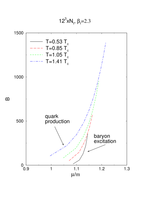
Figure 1: The number $B$ of Baryons which are present in the lattice universe as function of the chemical potential $\mu$ in units of the heavy quark mass $m$.

While the derivation of the effective gluonic action in the previous subsections holds for a SU($N_{c}$) gauge group, we will below confine ourselves to the case of a SU(2) gauge group. The partition function (58) supplemented with the action

$$-S_{latt} = \sum_{\{x\}}\biggl{(}\beta_{F}\,\sum_{\mu\nu}P_{\mu\nu}(x)\;+\;\xi\,\frac{1}{2}\,\hbox{tr}\,P(x)\biggr{)}\;,$$ (66)

$$\xi = \frac{2m^{3/2}T^{5/2}}{\sqrt{2}\pi^{3/2}}a^{4}\,\left[e^{\frac{\mu-m}{T}}\;+\;e^{-\frac{\mu+m}{T}}\,\right]$$ (67)

can be simulated with the standard heat bath algorithm of Creutz [19]. The non-locality of the action due to the Polyakov loops only yields a modest increase in computational time. We adjusted the temperature $T$ of the system by varying the number $N_{t}$ of lattice points in time direction, i.e., $T=1/N_{t}a$. In order to remove the superficial renormalization point, i.e., $\beta_{f}$, dependence from physical quantities, we assume that the one-loop scaling (47) is a good approximation for moderate $\beta_{f}$ values, i.e., $\beta_{f}\in[2.1,2.5]$. In order to fix the overall scales, we used

$$a(\beta_{f}=2.3)\;=\;0.16\,\hbox{ fm }\;,$$ (68)

which would correspond to a string tension of $\sigma=(440\,\hbox{MeV})^{2}$ in pure Yang-Mills theory $(N_{f}=0)$. The density of nuclear matter is roughly given by $\rho\approx 0.15\,\hbox{fm}^{-3}$. This value corresponds on average to $6\times 10^{-4}$ Baryons in an elementary cube of size $a^{3}$ and roughly one baryon in a lattice universe of size $12^{3}$.

In practice, it turned out to be convenient to run the simulation for a definite set of $\xi$-values, e.g. $\xi\in[0,1/2]$, and to calculate the relation between the parameters $\mu$, $m$, $T$ afterwards. The derivation of (66) relies on a truncation of the series (55) at $n=1$. For being consistent the inequality

$$\frac{1}{2^{5/2}}\;e^{-m/T}\;\frac{e^{2\mu/T}\,+\,e^{-2\mu/T}}{e^{\mu/T}\,+\,e^{\mu/T}}\;\left\langle|P|\right\rangle\;<\;1\;.$$ (69)

must be satisfied. In the present paper, we tacitly assume that the truncation at $n=1$ is reasonable if (69) is satisfied. Investigations beyond this approximation are left to future work.

4.1 Quark genesis versus quark confinement

In subsection 3.3, we have seen that in the deconfined phase $(\langle P\rangle={\cal O}(1))$ quarks can be produced in large numbers if the chemical potential exceeds the value of the quark mass. By contrast, in the ”confined” phase, i.e., $\langle P\rangle\approx 0$, the production of single quarks by means of the chemical potential is forbidden and only thermal excitations of baryons (i.e., diquarks for the present case of an SU(2) gauge theory) are possible. A large number of baryons is expected to occur for $\mu>2m-b$, where $m$ is the quark mass and $b$ is the binding energy of the diquark system. In order to study this interplay between quark production and confinement we have calculated the number $B$ of baryons which are present in the lattice universe as a function of the chemical potential for several temperatures. Pure Yang-Mills theory $(N_{f}=0)$ possesses a second order deconfimement phase transition for $T=T_{c}\approx 300\,$MeV. The result of the simulation using a $12^{3}\times N_{t}$ lattice and $\beta_{f}=2.3$ is shown in figure 1. For definiteness, we used $m=10\sqrt{\sigma}$. We have checked that the inequality (69) is satisfied for the parameter ranges producing figure 1. For temperatures below $T_{c}$, we clearly observe an onset value $\mu_{onset}$ larger than the quark mass. For temperatures larger $T_{c}$ a significant rise in the baryon number is observed for $\mu\approx m$. While in the previous case the net baryon number is produced via baryonic excitations, excitations of single quarks contribute to the net baryon number in the high temperature phase.

4.2 String breaking at finite density

Figure 2: schematic plot: the confinement order parameter (70) of pure SU(2) gauge theory in the case of a finite-density system as a function of the baryon density $\rho$ (left panel) and the chemical potential $\mu$ (right panel), respectively.

At zero baryon (quark) density, a convenient order parameter $O$ of confinement is constructed from the Polyakov line $P(\vec{x})$,

$$O\;:=\;\left\langle\left|\sum_{\{\vec{x}\}}P(\vec{x})\right|\right\rangle\;.$$ (70)

Keeping in mind that the Polyakov line reverses its sign under a center transformation, i.e., $P(\vec{x})\rightarrow-P(\vec{x})$, $\langle P(\vec{x})\rangle=0$ is mandatory for a realization of center symmetry. In this case, quark confinement is inherent [20] and one observes $O\propto 1/\sqrt{V}$, where $V$ is the space volume. If the temperature exceeds the critical temperature $T_{c}$ ($\approx 300\,$MeV for a pure SU(2) gauge theory), a non-vanishing expectation value of the Polyakov line, i.e., $\langle P(x)\rangle\not=0$ and therefore $O={\cal O}(1)$, signals the spontaneous breakdown of center symmetry and deconfinement.

While at zero density the color electric string between static quark sources might extend to arbitrary length, one expects at finite densities a maximum length $l_{0}$ of the color electric string which is controlled by the average distance between the background quarks. In this case, string breaking occurs and the heavy quark potential saturates at a quark distance $l_{0}$. A precise definition of a deconfinement order parameter is cumbersome in the finite density case, and has been under debate for more than twenty years (for recent progress see [22]).

Although one does not expect a sharp deconfinement phase transition as a function of temperature at finite densities, the gluonic state might undergo drastic changes which are triggered by temperature effects and which are signaled by significant (but smooth) changes in observables. To these respects, the behavior of $O$ is of particular interest also at finite densities. In the present case of an SU(2) gauge group ($\hbox{tr}\,P=\hbox{tr}\,P^{\dagger}$) and a system of heavy quarks, the density (60) is proportional to the expectation value of the Polyakov loop. One therefore finds

$$|\rho|\;\propto\;\left|\left\langle\hbox{tr}\,P\right\rangle\right|\;\leq\;\left\langle\left|\hbox{tr}\,P\right|\right\rangle\;,$$ (71)

and concludes that $O={\cal O}(1)$ as long as $\rho\not=0$. Our result nicely confirms the observation in [10] that color electric string breaking occurs as soon as the baryon density is non-zero.

We are led to the following behavior of $O$ as function of the chemical potential and density, respectively: for temperatures significantly below the critical temperature and for $\mu<\mu_{onset}$, the baryon density is practically zero yielding small values of $O$. If the chemical potential $\mu$ exceeds $\mu_{onset}$, the drastic rise of the density is accompanied by a strong increase of $O$. At large temperatures $(T>T_{c})$, $O$ is non-zero due to temperatures effects and changes in $O$ due to density effects are moderate in this case (see figure 2). Numerous numerical results confirm the qualitative behavior shown in figure 2. Quantitative details are not interesting since they strongly depend on the actual choice $m\gg\sqrt{\sigma}$ and on the fine tuning $\mu\rightarrow m^{+}$.

5 Conclusions

Our central idea of the present paper is to combine analytic methods for calculating the fermion determinant with the lattice description for deriving a valuable description of the Yang-Mills system at finite densities. Removing the ultra-violet regularization ($\Lambda\rightarrow\infty$ in the case of the quark determinant and $a\rightarrow 0$ in the case of the gluonic functional integral), physical quantities are independent of the type of regularization and approach a unique result. We have shown in section 3.2 how the proper scaling towards the continuum limit is obtained in the present case of interest. The advantage of our approach is twofold: firstly, by construction the approach is not plagued with spurious quark states (see e.g. [7]). Secondly, the physical heavy mass limit, i.e., $\Lambda_{YM},\,T\ll m\ll\Lambda$, is manifest.

In the case of the grand-canonical partition function, the chemical potential is chosen of the order of the quark mass in order to produce significant effects in the quark density [9]. Our first numerical results for the case of an SU(2) gauge group have been presented in section 4. Rising the temperature above the deconfinement critical one we observe a decrease of the onset value of the chemical potential at which a rapid increase of baryon density is observed. We interpret this result as follows: at low temperatures, baryon density is generated by the chemical potential only via the production of baryons (i.e., diquarks in the case of an SU(2) gauge group). At high temperatures, by contrast, the excitation of single quarks contributing to the density becomes feasible due to deconfinement.

In the case of the canonical partition function $Z(B)$, describing a system with baryon number $B$, we observe that the quark determinant is expressed in terms of products of Polyakov loops. In agreement with the findings in [10], the determinant is center symmetric, and a non-vanishing expectation value of the Polyakov loop at finite densities occurs via string breaking [10].

Although the calculation of the quark determinant in the present paper is tied to the Schwinger proper-time approach which generates the large mass expansion, the basic idea of combining an analytic calculation of the determinant with a subsequent lattice representation of the gluon fields is quite universal. Estimating fermion determinants by resorting to different types of approximation schemes has a long history in the literature. The idea of studying the opposite limit $m\rightarrow 0$ (chiral limit) by applying this new idea seems very appealing to us.

Acknowledgments:

We thank Mannque Rho and Dong-Pil Min for helpful discussions and encouragement. KL is indebted to Holger Gies for interesting discussions on fermion determinants in Schwinger proper-time regularization. We greatly acknowledge the hospitality of KIAS where large parts of the present work was performed. We thank C. W. Kim, President of KIAS, who made this collaboration possible.

Appendix A Notation and conventions

The metric tensor in Minkowski space is

$$g_{\mu\nu}\;=\;\hbox{diag}(1,-1,-1,-1)\;.$$ (A.1)

We define Euclidean tensors $T_{(E)}$ from the tensors in Minkowski space $T_{(M)}$ by

$$T^{\mu_{1}\ldots\mu_{N}}_{(E)\phantom{\ldots\mu_{N}}\nu_{1}\ldots\nu_{n}}\;=\;(i)^{r}\,(-i)^{s}\;T^{\mu_{1}\ldots\mu_{N}}_{(M)\phantom{\ldots\mu_{N}}\nu_{1}\ldots\nu_{n}}\;,$$ (A.2)

where $r$ and $s$ are the numbers of zeros within $\{\mu_{1}\ldots\mu_{N}\}$ and $\{\nu_{1}\ldots\nu_{n}\}$, respectively. In particular, we have for the Euclidean time and the Euclidean metric

$$x_{(E)}^{0}\;=\;i\,x_{(M)}^{0}\;,\hbox to28.45274pt{\hfill}g^{\mu\nu}_{(E)}\;=\;\hbox{diag}(-1,-1,-1,-1)\;.$$ (A.3)

Covariant and contra-variant vectors in Euclidean space differ by an overall sign. For a consistent treatment of the symmetries, one is forced to consider the $\gamma^{\mu}$ matrices as vectors. Therefore, one is naturally led to anti-hermitian Euclidean matrices via (A.2),

$$\gamma^{0}_{(E)}=i\gamma^{0}_{(M)}\;,\hbox to28.45274pt{\hfill}\gamma^{k}_{(E)}=\gamma^{k}_{(M)}\;.$$ (A.4)

In particular, one finds

$$\left(\gamma^{\mu}_{(E)}\right)^{\dagger}\;=\;-\;\gamma^{\mu}_{(E)}\;,\hbox to28.45274pt{\hfill}\{\gamma^{\mu}_{(E)},\gamma^{\nu}_{(E)}\}\;=\;2g^{\mu\nu}_{(E)}\;=\;-2\,\delta_{\mu\nu}\;.$$ (A.5)

The so-called Wick rotation is performed by considering the Euclidean tensors (A.2) as real fields.

In addition, we define the square of an Euclidean vector field, e.g. $V_{\mu}$, by

$$V^{2}\;:=\;V_{\mu}V_{\mu}\;=\;-V_{\mu}V^{\mu}\;.$$ (A.6)

This implies that $V^{2}$ is always a positive quantity (after the wick rotation to Euclidean space).

Appendix B The off-diagonal heat coefficients

Figure 3: Possibilities (a) and (b) for calculating the holonomy along the triangle path shown in (a) (non-Abelian Stokes theorem).

The aim of this subsection is to calculate the full space time dependence of the heat coefficients $h_{k}(x,y)$. We will show that we recover the well known result for the diagonal part $h_{k}(x,x)$. For this purpose, our starting point is the recursion relation

$$(k+z_{\mu}D_{\mu})h_{k}(x,y)=(D^{2}+{i\over 2}\sigma_{\mu\nu}[D_{\mu},D_{\nu}])h_{k-1}(x,y)\;,$$ (B.1)

while the equation for $h_{0}(x,y)$ is given by

$$z_{\mu}D_{\mu}h_{0}(x,y)=0\;,\hbox to28.45274pt{\hfill}z_{\mu}\,:=\,x_{\mu}-y_{\mu}\;.$$ (B.2)

We first show that the gauge covariant connection

$$h_{0}(x,y)\;=\;U(x,y)\;=\;{\cal P}\exp\left\{-i\int_{C_{xy}}A_{\mu}(x^{\prime})\;dx_{\mu}^{\prime}\,\right\}$$ (B.3)

where the path $C_{xy}$ is a straight line connecting the points $x$ and $y$, provides a solution to equation (B.2). For a proof we calculate the holonomy along the triangle path shown in figure 3. By a comparison of the results obtained by using the equivalent paths (a) and (b) in figure 3 at the level ${\cal O}(dx)$, one finds

$$U^{\dagger}(x,y)\,D_{\mu}U(x,y) = -i\,\int_{0}^{1}\;dt\;t\,z_{\nu}\;{\cal F}_{\mu\nu}(zt+y,y)\;,$$ (B.4)

$${\cal F}_{\mu\nu}(x^{\prime},y) := U^{\dagger}(x^{\prime},y)\;F_{\mu\nu}(x^{\prime})\;U(x^{\prime},y)\;.$$ (B.5)

In the Abelian case ${\cal F}_{\mu\nu}(x^{\prime},y)$ becomes independent of $y$ and coincides with the standard field strength $F_{\mu\nu}(x^{\prime})$. It is can be easily checked that both sides of (B.4) transform homogeneously under gauge transformations. Using (B.5) and the anti-symmetry of the tensor ${\cal F}_{\mu\nu}(x^{\prime},y)$ under an exchange of the indices $\mu$ and $\nu$, one immediately observes that $z_{\mu}D_{\mu}h_{0}(x,y)=0$.

In order to calculate the heat coefficients $h_{k}(x,y)$, we decompose

$$h_{k}(x,y)\;=\;U(x,y)\,g_{k}(x,y)\;,\hbox to85.35826pt{\hfill with \hfill}g_{0}(x,y)\;=\;1\;.$$

Making extensive use of (B.4) and the relation

$$D_{\mu}\,\biggl{(}U(x,y)\,g_{k}(x,y)\biggr{)}\;=\;\biggl{(}D_{\mu}\,U(x,y)\biggr{)}\,g_{k}(x,y)\;+\;U(x,y)\,\biggl{(}\partial_{\mu}g_{k}(x,y)\biggr{)}\;,$$

one can cast (B.1) into a recursion relation for $g_{k}(x,y)$, i.e.,

$$(k+z_{\mu}\partial_{\mu})\hbox to0.0pt{$\displaystyle g_{k}(x,y)$\hss}$$ (B.6)

$$= \left(\partial^{2}-{2i\over z}\int_{C_{xy}}z^{\prime}dx^{\prime}_{\alpha}{\cal F}_{\mu\alpha}(x^{\prime},y)\partial_{\mu}\right.$$

$$-{1\over z^{2}}\int_{C_{xy}}z^{\prime}dx^{\prime}_{\alpha}{\cal F}_{\mu\alpha}(x^{\prime},y)\int_{C_{xy}}z^{\prime\prime}dx^{\prime\prime}_{\beta}{\cal F}_{\mu\beta}(x^{\prime\prime},y)$$

$$-{i\over z^{2}}\int_{C_{xy}}z^{\prime 2}dx^{\prime}_{\alpha}\partial^{\prime}_{\mu}{\cal F}_{\mu\alpha}(x^{\prime},y)-{\sigma_{\mu\nu}\over z^{2}}\int_{C_{xy}}z^{\prime}_{\alpha}dx^{\prime}_{\alpha}{\cal F}_{\mu\nu}(x^{\prime},y)$$

$$-{i\sigma_{\mu\nu}\over 2z^{2}}\int_{C_{xy}}z^{\prime}dx^{\prime}_{\alpha}\int_{C_{xy}}z^{\prime\prime}dx^{\prime\prime}_{\beta}[{\cal F}_{\mu\alpha}(x^{\prime},y),{\cal F}_{\nu\beta}(x^{\prime\prime},y)]$$

$$+\left.{\sigma_{\mu\nu}\over 2z^{2}}\int_{C_{xy}}z^{\prime 2}dx^{\prime}_{\alpha}(\partial^{\prime}_{\mu}{\cal F}_{\nu\alpha}(x^{\prime},y)-\partial^{\prime}_{\nu}{\cal F}_{\mu\alpha}(x^{\prime},y))\right)g_{k-1}(x,y)\;.$$

In particular, the equation for $g_{1}(x,y)$ becomes

$$(1+z_{\mu}\partial_{\mu})g_{1}(x,y\hbox to0.0pt{$\displaystyle)=-{1\over z^{2}}\int_{C_{xy}}z^{\prime}dx^{\prime}_{\alpha}{\cal F}_{\mu\alpha}(x^{\prime},y)\int_{C_{xy}}z^{\prime\prime}dx^{\prime\prime}_{\beta}{\cal F}_{\mu\beta}(x^{\prime\prime},y)$\hss}$$ (B.7)

$$-{i\over z^{2}}\int_{C_{xy}}z^{\prime 2}dx^{\prime}_{\alpha}\partial^{\prime}_{\mu}{\cal F}_{\mu\alpha}(x^{\prime},y)-{\sigma_{\mu\nu}\over z^{2}}\int_{C_{xy}}z^{\prime}_{\alpha}dx^{\prime}_{\alpha}{\cal F}_{\mu\nu}(x^{\prime},y)$$

$$-{i\sigma_{\mu\nu}\over 2z^{2}}\int_{C_{xy}}z^{\prime}dx^{\prime}_{\alpha}\int_{C_{xy}}z^{\prime\prime}dx^{\prime\prime}_{\beta}[{\cal F}_{\mu\alpha}(x^{\prime},y),{\cal F}_{\nu\beta}(x^{\prime\prime},y)]$$

$$+{\sigma_{\mu\nu}\over 2z^{2}}\int_{C_{xy}}z^{\prime 2}dx^{\prime}_{\alpha}(\partial^{\prime}_{\mu}{\cal F}_{\nu\alpha}(x^{\prime},y)-\partial^{\prime}_{\nu}{\cal F}_{\mu\alpha}(x^{\prime},y))$$

Referring to the particular solution of the equation $(k+z_{\mu}\partial_{\mu})A(x,y)=B(x,y)$ given by

$$A(x,y)={1\over z^{k}}\int_{C_{xy}}z^{\prime k-2}\,z^{\prime\mu}B(x,y)dx^{\prime\mu}$$ (B.8)

we finally obtain

$$g_{1}(x,y)=-{1\over z}\int_{C_{xy}}z^{\prime-1}z^{\prime}_{\lambda}dx^{\prime}_{\lambda}\hbox to0.0pt{$\displaystyle\left({1\over z^{\prime 2}}\int_{C_{x^{\prime}y}}z^{\prime\prime}dx^{\prime\prime}_{\alpha}{\cal F}_{\mu\alpha}(x^{\prime\prime},y)\int_{C_{x^{\prime}y}}z^{\prime\prime\prime}dx^{\prime\prime\prime}_{\beta}{\cal F}_{\mu\beta}(x^{\prime\prime\prime},y)\right.$\hss}$$

$$+{i\over z^{\prime 2}}\int_{C_{x^{\prime}y}}z^{\prime\prime 2}dx^{\prime\prime}_{\alpha}\partial^{\prime\prime}_{\mu}{\cal F}_{\mu\alpha}(x^{\prime\prime},y)$$

$$+{\sigma_{\mu\nu}\over z^{\prime 2}}\int_{C_{x^{\prime}y}}z^{\prime\prime}_{\alpha}dx^{\prime\prime}_{\alpha}{\cal F}_{\mu\nu}(x^{\prime\prime},y)$$

$$+{i\sigma_{\mu\nu}\over 2z^{\prime 2}}\int_{C_{x^{\prime}y}}z^{\prime\prime}dx^{\prime\prime}_{\alpha}\int_{C_{x^{\prime}y}}z^{\prime\prime\prime}dx^{\prime\prime\prime}_{\beta}[{\cal F}_{\mu\alpha}(x^{\prime\prime},y),{\cal F}_{\nu\beta}(x^{\prime\prime\prime},y)]$$

$$-\left.{\sigma_{\mu\nu}\over 2z^{\prime 2}}\int_{C_{x^{\prime}y}}z^{\prime\prime 2}dx^{\prime\prime}_{\alpha}(\partial^{\prime\prime}_{\mu}{\cal F}_{\nu\alpha}(x^{\prime\prime},y)-\partial^{\prime\prime}_{\nu}{\cal F}_{\mu\alpha}(x^{\prime\prime},y))\right)$$

Not showing terms which vanish if the trace over Dirac indices is performed, we find

$$h_{1}(x,y) = -{\cal P}\,\exp\left\{-i\int_{C_{xy}}A_{\mu}(x^{\prime})\;dx_{\mu}^{\prime}\,\right\}\frac{1}{z}\int_{C_{xy}}z^{\prime-1}z^{\prime}_{\lambda}\;dx^{\prime}_{\lambda}$$ (B.10)

$$\frac{1}{z^{\prime 2}}\int_{C_{x^{\prime}y}}z^{\prime\prime}\;dx^{\prime\prime}_{\alpha}\;{\cal F}_{\mu\alpha}(x^{\prime\prime},y)\int_{C_{x^{\prime}y}}z^{\prime\prime\prime}\;dx^{\prime\prime\prime}_{\beta}\;{\cal F}_{\mu\beta}(x^{\prime\prime\prime},y)\;+\;\ldots\;.$$

For calculating $g_{2}(x,y)$, we introduce

$$x^{\prime}=zp+y,\,x^{\prime\prime}=z^{\prime}t+y=zpt+y,\,x^{\prime\prime\prime}=z^{\prime}s+y=zps+y$$

and rewrite $g_{1}(x,y)$ as

$$g_{1}(x,y)=\hbox to0.0pt{$\displaystyle-\int_{0}^{1}p^{2}dp\int_{0}^{1}tdt\int_{0}^{1}sdsz_{\alpha}z_{\beta}{\cal F}_{\mu\alpha}(zpt+y,y){\cal F}_{\mu\beta}(zps+y,y)$\hss}$$ (B.11)

$$-i\int_{0}^{1}dp\int_{0}^{1}tdtz_{\alpha}\partial_{\mu}{\cal F}_{\mu\alpha}(zpt+y,y)$$

$$-\sigma_{\mu\nu}\int_{0}^{1}dp\int_{0}^{1}tdt{\cal F}_{\mu\nu}(zpt+y,y)$$

$$-{i\sigma_{\mu\nu}\over 2}\int_{0}^{1}p^{2}dp\int_{0}^{1}tdt\int_{0}^{1}sdsz_{\alpha}z_{\beta}[{\cal F}_{\mu\alpha}(zpt+y,y),{\cal F}_{\nu\beta}(zps+y,y)]$$

$$+{\sigma_{\mu\nu}\over 2}\int_{0}^{1}dp\int_{0}^{1}tdtz_{\alpha}(\partial_{\mu}{\cal F}_{\nu\alpha}(zpt+y,y)-\partial_{\nu}{\cal F}_{\mu\alpha}(zpt+y,y))$$

where $\partial_{\mu}{\cal F}_{\mu\nu}(zpt+y,y)=\partial_{\mu}{\cal F}_{\mu\nu}(x,y)|_{x=zpt+y}$. Using (B.6), (B.8) and (B.11), the final result of a lengthy calculation is

$$g_{2}(x,y)\hbox to0.0pt{$\displaystyle=\frac{1}{z^{2}}\int_{C_{xy}}z^{\prime}_{\gamma}\;dx^{\prime}_{\gamma}\left\{-\int_{0}^{1}p^{2}dp\int_{0}^{1}tdt\int_{0}^{1}sds\biggl{(}2{\cal F}_{\mu\nu}(z^{\prime}pt+y,y){\cal F}_{\mu\nu}(z^{\prime}ps+y,y)\right.$\hss}$$ (B.12)

$$\hskip 85.35826pt+2z^{\prime}_{\beta}\partial^{\prime}_{\lambda}(\{{\cal F}_{\mu\lambda}(z^{\prime}pt+y,y),{\cal F}_{\mu\beta}(z^{\prime}ps+y,y)\})$$

$$\hskip 85.35826pt+z^{\prime}_{\alpha}z^{\prime}_{\beta}\partial^{\prime 2}{\cal F}_{\mu\alpha}(z^{\prime}pt+y,y){\cal F}_{\mu\beta}(z^{\prime}ps+y,y)\biggr{)}$$

$$+2\left(\int_{0}^{1}dp\int_{0}^{1}tdt{\cal F}_{\mu\nu}(z^{\prime}pt+y,y)\right.$$

$$+{i\over 2}\int_{0}^{1}p^{2}dp\int_{0}^{1}tdt\int_{0}^{1}sdsz^{\prime}_{\alpha}z^{\prime}_{\beta}[{\cal F}_{\mu\alpha}(z^{\prime}pt+y,y),{\cal F}_{\nu\beta}(z^{\prime}ps+y,y)]$$

$$-\left.{1\over 2}\int_{0}^{1}dp\int_{0}^{1}tdtz^{\prime}_{\alpha}(\partial^{\prime}_{\mu}{\cal F}_{\nu\alpha}(z^{\prime}pt+y,y)-\partial_{\nu}{\cal F}_{\mu\alpha}(z^{\prime}pt+y,y))\right)^{2}\biggr{\}}\;+\;\ldots\;,$$

where we have not shown the traceless terms. In the diagonal limit $x\rightarrow y$, the formulas for $g_{1}(x,y)$ and $g_{2}(x,y)$ greatly simplify and we recover the familiar result

$$g_{1}(x,x) = 0$$

$$g_{2}(x,x) = -{1\over 12}F^{2}+{1\over 8}F^{2}$$ (B.13)

$$= {1\over 6}F^{2}\;.$$

References

• [1] K. Kanaya, Prog. Theor. Phys. Suppl. 131 (1998) 73.
• [2] S. Duane, A. D. Kennedy, B. J. Pendleton and D. Roweth, Phys. Lett. B195 (1987) 216;
S. Duane and J. B. Kogut, Nucl. Phys. B275 (1986) 398.
• [3] S. Hands, J.B. Kogut, M. Lombardo and S. E. Morrison, Symmetries and spectrum of SU(2) lattice gauge theory at finite chemical potential , hep-lat/9902034.
• [4] I. M. Barbour, A.J. Bell, M. Bernaschi, G. Salina and A. Vladikas, Nucl. Phys. B386 (1992) 683.
• [5] I. M. Barbour, talk presented at Workshop on QCD at Finite Baryon Density: A Complex System with a Complex Action, Bielefeld, Germany, 27-30 Apr 1998.
• [6] I. Barbour, N. Behilil, E. Dagotto, F. Karsch, A. Moreo, M. Stone and H.W. Wyld, Nucl. Phys. B275 (1986) 296.
• [7] M. A. Stephanov, Phys. Rev. Lett. 76 (1996) 4472.
• [8] I. Bender, T. Hashimoto, F. Karsch, V. Linke, A. Nakamura, M. Plewnia, I. O. Stamatescu, W. Wetzel, Nucl. Phys. Proc. Suppl. 26 (1992) 323.
• [9] T. C. Blum, J. E. Hetrick and D. Toussaint, Phys. Rev. Lett. 76 (1996) 1019.
• [10] O. Kaczmarek, J. Engels, F. Karsch and E. Laermann, “Lattice QCD at nonzero baryon number,” hep-lat/9905022.
J. Engels, O. Kaczmarek, F. Karsch and E. Laermann, “The Quenched limit of lattice QCD at nonzero baryon number,” hep-lat/9903030.
• [11] D. E. Miller and K. Redlich, Phys. Rev. D37 (1988) 3716.
• [12] F. J. Yndurain, ’Quantum Chromodynamics’, Springer Verlag, 1983.
• [13] K. G. Wilson, Phys. Rev. B4 (1971) 3174;
K. G. Wilson and J. Kogut, Phys. Rept. 12 (1974) 75.
• [14] T. Appelquist and J. Carrazzone, Phys. Rev. D11 (1975) 2865.
• [15] KL greatly acknowledges helpful discussions with Holger Gies.
• [16] D. Ebert, H. D Reinhardt, Nucl. Phys. B271 (1986) 188.
• [17] P. Elmfors, D. Persson and B. Skagerstam, Astropart. Phys. 2 (1994) 299.
• [18] H. Gies, QED effective action at finite temperature, hep-ph/9812436, in press by Phys. Rev. D.
• [19] M. Creutz, Phys. Rev. D21 (1980) 2308.
• [20] B. Svetitsky, Phys. Rep. 132 (1986) 1.
• [21] P.d. Forcrand and V. Laliena, The role of the polyakov loop in finite density QCD, hep-lat/9907004.
• [22] H. Satz, Nucl. Phys. A642 (1998) 130.