Chiral Fermions and Multigrid

Abstract

Lattice regularization of chiral fermions is an important development of the theory of elementary particles. Nontheless, brute force computer simulations are very expensive, if not prohibitive. In this letter I exploit the non-interacting character of the lattice theory in the flavor space and propose a multigrid approach for the simulation of the theory. Already a two-grid algorithm saves an order of magnitude of computer time for fermion propagator calculations.

PACS No.: 11.15Ha, 11.30.Rd, 11.30.Fs

Key Words: Lattice QCD, Chiral fermions, Algorithms

1 Introduction

After many years of research in lattice QCD, it was possible to formulate QCD with chiral fermions on the lattice [1, 2, 3, 4].

The basic idea is an expanded flavor space which may be seen as an extra dimension with left and right handed fermions defined in the two opposite boundaries or walls.

Let $N$ be the size of the extra dimension, $D_{W}$ the Wilson-Dirac operator, and $m$ the bare fermion mass. Then, the theory with Domain Wall fermions is defined by the action [1, 2]:

$$\begin{array}[]{l}S_{DW}:=\bar{\Psi}{\cal{M}}\Psi=\sum_{i=1}^{N}\bar{\psi}_{i}[(D^{||}-1)\psi_{i}+P_{+}\psi_{i+1}+P_{-}\psi_{i-1}]\\ P_{+}(\psi_{N+1}+m\psi_{1})=0,~{}~{}P_{-}(\psi_{0}+m\psi_{N})=0\end{array}$$ (1)

where $\cal{M}$ is the five-dimensional fermion matrix of the regularized theory and $D^{||}=M-D_{W}$ with $M\in(0,2)$ being a mass parameter.

I define also a theory with Truncated Overlap Fermions in complete analogy with the domain wall fermions by substituting [5]:

$$P_{+}\rightarrow(D^{||}+1)P_{+},~{}~{}P_{-}\rightarrow(D^{||}+1)P_{-}$$ (2)

Both theories can be compactified in the walls of the extra fifth dimension as low energy effective theories given by the action:

$$\begin{array}[]{l}S_{eff}=\bar{\chi}_{1}D\chi_{1}\\ \chi_{1}=P_{+}\psi_{1}+P_{-}\psi_{N},~{}~{}\bar{\chi}_{1}=\bar{\psi}_{1}P_{-}+\bar{\psi}_{N}P_{+}\end{array}$$ (3)

where $D$ is the chiral Dirac operator satisfying the Ginsparg-Wilson relation [6]:

$$\gamma_{5}D^{-1}+D^{-1}\gamma_{5}=a\gamma_{5}R,$$ (4)

where $a$ is the lattice spacing and $R$ is a local operator trivial in the Dirac space.

I defined Truncated Overlap Fermions such that in the large $N$ limit one obtains Overlap Fermions [3] with the Dirac operator given by [7]:

$$D_{OV}=\frac{1+m}{2}-\frac{1-m}{2}\gamma_{5}\mbox{sgn}(H)$$ (5)

where $H=\gamma_{5}D^{||}$.

Untill now, the computations with chiral fermions with the standard algorithms have been very expensive. The extra fermion flavors introduce a large overhead. One multiplication with the fermion matrix costs ${\cal{O}}(n)$ $D_{W}$-multiplications with $n\sim N$ for domain wall fermions and much larger for the overlap operator [8, 9, 10].

In this letter I propose a multigrid algorithm along the fifth dimension which makes these simulations much faster. The key observation is the lack of gauge connections along this dimension. It is well-known that the overhead of such algorithms scales like $N$log$N$.

Here it is the $multigrid$ algorithm: ALGORITHM1 (Generic) for solving the system $D_{OV}x=b$:

$$\begin{array}[]{l}\mbox{Given}~{}N,~{}x_{0},~{}r_{0}(=b),~{}tol,~{}tol_{1},~{}\mbox{set}~{}tol_{0}=1~{}\mbox{and iterate:}\\ for~{}i=1,\ldots\\ ~{}~{}~{}~{}tol_{0}=tol_{0}tol_{1}\\ ~{}~{}~{}~{}\mbox{Solve}~{}Dy=r_{i-1}~{}\mbox{within}~{}tol_{0}\\ ~{}~{}~{}~{}x_{i}=x_{i-1}+y\\ ~{}~{}~{}~{}r_{i}=b-D_{OV}x_{i}\\ ~{}~{}~{}~{}if||r_{i}||_{2}<tol,~{}end~{}for\\ \end{array}$$ (6)

where by $o$ is denoted a vector with zero entries and $tol_{1},tol$ are tolerances. $tol_{1}$ is typically orders of magnitude larger than $tol$ such that the work per $D_{OV}$ inversion is minimized.

Remark 1. The straightforward application of the $ALGORITHM1$ gives a two-grid algorithm. By calling it again in solving the smaller system and iterating, one gets a full multigrid algorithm.

Remark 2. The corresponding Hybrid Monte Carlo (HMC) algorithm can be obtained by working with an approximate Hamiltonian in the coarse lattice and by a global correction on the fine lattice.

In Fig. 1 we compare the norm of the residual $r_{i}=b-D_{OV}x_{i}$ of the Conjugate Residual (CR) algorithm (which is optimal since $D_{OV}$ is normal [11]) and $ALGORITHM1$. I gain about an order of magnitude (in average) on $30$ $4^{4}$-configurations at $\beta=6.0$ and $m=0.1$.

For the coarse lattice we used $N=6$ with the Truncated Overlap Fermions and the Lanczos method to compute $D_{OV}$ [8].

Let $P$ be the following orthogonal transformation:

$$\chi_{i}=P_{+}\psi_{i}+P_{-}\psi_{i-1}$$ (7)

I computed the inverse of $D$ in the $ALGORITHM1$ using

$$D^{-1}=(P^{T}{\cal{M}}^{-1}{\cal{M}}_{1}P)_{1,1}$$ (8)

where ${\cal{M}}_{1}$ is the same as $\cal{M}$ but with $m=1$ [5] and the subscript $1,1$ stands for the $(1,1)$ block of an $N$x$N$ partitioned matrix along the fifth dimension.

Recently, the possibility of a Multigrid algorithm along the all dimensions is raised [12]. In this case a gauge fixing is needed.

I would like to thank Philippe de Forcrand for suggestions on how to improve the $ALGORITHM1$ and Herbert Neuberger for interesting discussions after my talk at Lattice99 conference.

The author thanks PSI where this work was done and SCSC Manno for the allocation of computer time on the NEC SX4.

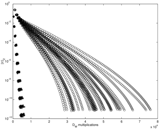
Figure 1: Norm of the residual error vs. the number of $D_{W}$ multiplications on 30 configurations. Circles stand for the straightforward inversion with CR and stars for the $ALGORITHM1$.

References

- [1] D.B. Kaplan, Phys. Lett. B 228 (1992) 342.
- [2] Y. Shamir, Nucl. Phys. B 406 (1993) 90; V. Furman and Y. Shamir, Nucl. Phys. B (1995) 54.
- [3] R. Narayanan, H. Neuberger, Phys. Lett. B 302 (1993) 62, Nucl. Phys. B 443 (1995) 305.
- [4] P. Hasenfratz, V. Laliena and F. Niedermayer, Phys. Lett. B 427 (1998) 125.
- [5] A. Boriçi, Truncated Overlap Fermions, Talk at The XVII International Symposium in Lattice Field Theory, Pisa, June 29 - July 3, 1999.
- [6] P. H. Ginsparg and K. G. Wilson, Phys. Rev. D 25 (1982) 2649.
- [7] H. Neuberger, Phys. Lett. B 417 (1998) 141, Phys. Rev. D 57 (1998) 5417.
- [8] A. Boriçi, Phys. Lett. B 453 (1999) 46.
- [9] H. Neuberger, Phys. Rev. Lett. 81 (1998) 4060.
- [10] R. G. Edwards, U. M. Heller and R. Narayanan, FSU-SCRI-98-71, and hep-lat/9807017.
- [11] A. Boriçi, Krylov Subspace Methods in Lattice QCD, PhD Thesis, CSCS TR-96-27, ETH Zürich 1996.
- [12] , L. Giusti, Ch. Hoelbling and C. Rebbi, hep-lat/9906004.