Exact fermion zero-mode for the new calorons ITEP-TH-27/99; INLO-PUB-13/99

Abstract

We construct the fermion zero-mode for arbitrary charge one $SU(n)$ calorons with non-trivial holonomy, both in the finite temperature context (anti-periodic boundary conditions in time) and in the Kaluza-Klein compactification context (periodic boundary conditions in time). The zero-mode is localised on one of the constituent monopoles and we discuss a relation to the Callias index theorem.

1 Introduction

The $SU(n)$ instantons at finite temperature (or calorons) can be seen as bound states of $n$ constituent monopoles, evident only when the Polyakov loop at spatial infinity is non-trivial. In the periodic gauge, $A_{\mu}(t\!+\!{\beta},\vec{x})\!=\!\!A_{\mu}(t,\vec{x})$,

$${{\cal P}_{\infty}}=\lim_{|\vec{x}|\rightarrow\infty}P\,\exp(\int_{0}^{\beta}A_{0}(\vec{x},t)dt).$$ (1)

After a suitable constant gauge transformation, it can be characterised by $\sum_{m=1}^{n}\mu_{m}\!=\!0$ and

$${{\cal P}_{\infty}^{0}}=\exp[2\pi i\,{\rm diag}(\mu_{1},\ldots,\mu_{n})],$$ (2)

$$\mu_{1}\leq\ldots\leq\mu_{n}\leq\mu_{n+1}\!\equiv\!1\!+\!\mu_{1}.$$

Using the classical scale invariance we can always arrange $\beta=1$, as will be assumed throughout. A remarkably simple formula for the $SU(n)$ action density exists [1, 2].

$${\rm Tr}F_{\mu\nu}^{\,2}(x)=\partial_{\mu}^{2}\partial_{\nu}^{2}\log\psi(x),$$ (3)

$$\psi(x)={\scriptstyle{{1\over 2}}}{\rm tr}({\cal{A}}_{n}\cdots{\cal{A}}_{1})-\cos(2\pi t),$$

$${\cal{A}}_{m}\equiv\frac{1}{r_{m}}\left(\!\!\!\begin{array}[]{cc}r_{m}\!\!&|\vec{y}_{m}\!\!-\!\vec{y}_{m+1}|\\ 0\!\!&r_{m+1}\end{array}\!\!\!\right)\left(\!\!\!\begin{array}[]{cc}c_{m}\!\!&s_{m}\\ s_{m}\!\!&c_{m}\end{array}\!\!\!\right),$$ (8)

with $r_{m}\!=\!|\vec{x}\!-\!\vec{y}_{m}|$ the center of mass radius of the $m^{\rm th}$ constituent monopole, which can be assigned a mass $8\pi^{2}\nu_{m}$, where $\nu_{m}\!\equiv\!\mu_{m+1}\!-\!\mu_{m}$. Furthermore, $c_{m}\!\equiv\!\cosh(2\pi\nu_{m}r_{m})$, $s_{m}\!\equiv\!\sinh(2\pi\nu_{m}r_{m})$, $r_{n+1}\!\equiv\!r_{1}$ and $\vec{y}_{n+1}\!\equiv\!\vec{y}_{1}$.

2 Monopole constituents

These generalised caloron solutions can be found [3] using a combination of the Nahm transformation [4] and the Atiyah-Drinfeld-Hitchin-Manin (ADHM) construction [5]. The latter is mainly needed to resolve the delta function singularities that arise in the Nahm transformation, although other methods were developed as well [6].

The Nahm equation for these charge one instantons reduces to an abelian problem on the circle, parametrised by $z$ mod 1,

$$\frac{d}{dz}\hat{A}_{j}(z)=2\pi i\sum_{m}\left(y_{m}^{j}-y_{m-1}^{j}\right)\delta(z-\mu_{m}),$$ (9)

giving $\hat{A}_{j}(z)=2\pi iy_{m}^{j}$, for $z\in[\mu_{m},\mu_{m+1}]$. In the monopole literature $\hat{A}_{j}(z)$ is usually denoted by $T_{j}(z)$. Taking one interval in isolation, applying the Nahm transformation [4] gives a single static Bogomol’nyi-Prasad-Sommerfeld (BPS) monopole with mass proportional to the length ($\nu_{m}$) of the interval. Taking $|\vec{y}_{n}|\!\rightarrow\!\infty$ leaves the interval $[\mu_{1},\mu_{n}]$, allowing for the interpretation of an $SU(n)$ monopole with $\mu_{i}$ specifying the eigenvalues of the Higgs field at infinity, for which it is crucial they add to zero. Indeed, in the periodic gauge $A_{0}$ tends to a constant at spatial infinity.

Note that we have to order $\exp(2\pi i\mu_{m})$ along the circle to ensure that the $\nu_{i}$ add to 1, an ordering inherited by $\mu_{m}$ when extended to the real line by insisting $\mu_{kn+m}\!=\!k\!+\!\mu_{m}$, for any integer $k$. Let us pick one to be labelled by $\mu_{1}$. All we can guarantee at this point is that $\sum_{m=1}^{n}\mu_{m}=\ell$, an integer. With $\mu_{kn+m}\!=\!k\!+\!\mu_{m}$, we find $\sum_{m=1}^{n}\mu_{m+p}=\ell+p$, for any integer $p$. A cyclic shift of the labels by $p\!=\!-\ell$ proves that there is a unique choice of the $\mu_{m}$ that satisfy eq. (2). It demonstrates why $\vec{y}_{n}$ does play a special role, and in the limit $|\vec{y}_{n}|\!\rightarrow\!\infty$ one therefore has a static monopole solution [4], which can be seen as the composite of $n\!-\!1$ BPS monopoles of mass $\nu_{m}$, located at $\vec{y}_{m}$, for $m\!=\!1,\cdots,n\!-\!1$. From the general formalism it is clear these $n\!-\!1$ monopole constituents are time independent, as was verified explicitly for $SU(2)$ [2, 3]. Note that our argument demonstrates that for $|\vec{y}_{m}|\!\rightarrow\!\infty$ with $m\!\neq\!n$, one is left with a gauge field that cannot be time independent, even though the resulting action density is [2].

The significance of one constituent carrying a time dependent field lies in the fact that the $n$ constituent monopoles form an instanton, and the topological charge can be associated to the so-called Taubes-winding [7], described by a time dependent (gauge) rotation, going full circle when $t$ progresses over one period. For $SU(2)$ this can be read-off from the explicit expression for the gauge field [2, 3]. We thus conclude that the constituent located at $\vec{y}_{n}$ is the one that carries this Taubes-winding, even though its action density is time independent for well-separated constituents. This conclusion can also be drawn from the formalism developed in ref. [6], see also ref. [8].

3 Fermion zero-mode

The basic ingredient in the construction of caloron solutions is a Greens function defined by

$$\left(\!\!D_{z}^{2}\!+\!r^{2}(x;z)\!+\!\!\sum_{m}\!\delta_{m}(z)\!\right)\!\!\hat{f}_{x}(z,z^{\prime})\!=\!\delta(z\!-\!z^{\prime}),$$ (10)

where $D_{z}\!=\!(2\pi i)^{-1}\!\partial_{z}\!-\!t$, $r^{2}(x;z)\!=\!r_{m}^{2}(x)$ for $z\in[\mu_{m},\mu_{m+1}]$ and $\delta_{m}(z)=\delta(z\!-\!\mu_{m})|\vec{y}_{m}\!-\!\vec{y}_{m-1}|/2\pi$. A similarity with the impurity scattering problem allows for a straightforward solution [1], which we present here for the case that $\mu_{m}\!\leq\!z^{\prime}\!\leq\!z\!\leq\!\mu_{m+1}$ (extended to $z<z^{\prime}$ by $\hat{f}_{x}(z^{\prime},z)=\hat{f}_{x}^{*}(z,z^{\prime})$)

$$\hskip-8.53581pt\hat{f}_{z}(z,z^{\prime})\!=\!\!\frac{\pi e^{2\pi it(z\!-\!z^{\prime})}}{r_{m}\psi}\Bigl{(}e^{-2\pi it}\sinh\left(2\pi(z-z^{\prime})r_{m}\right)\!+\hskip-11.66563pt$$

$$<\!v_{m}(z^{\prime})|{\cal{A}}_{m\!-\!1}\cdots{\cal{A}}_{1}{\cal{A}}_{n}\cdots{\cal{A}}_{m}|w_{m}(z)\!>\!\Bigr{)},$$ (11)

where the spinors $v_{m}$ and $w_{m}$ are defined by

$$v_{m}^{1}(z)=-w_{m}^{2}(z)=\sinh\left(2\pi(z\!-\!\mu_{m})r_{m}\right),$$

$$v_{m}^{2}(z)=\hphantom{-}w_{m}^{1}(z)=\cosh\left(2\pi(z\!-\!\mu_{m})r_{m}\right).$$ (12)

For the zero-mode densities we find

$$|\Psi_{z}(x)|^{2}=-(2\pi)^{-2}\partial_{\mu}^{2}\hat{f}_{x}(z,z),$$ (13)

derived exactly as for $SU(2)$ [9], not repeated here. With the gauge field in the periodic gauge one has, $\Psi_{z}(t\!+\!1,\vec{x})=\exp(2\pi iz)\Psi_{z}(t,\vec{x})$. To obtain the finite temperature fermion zero-mode one puts $z={\scriptstyle{{1\over 2}}}$, whereas for the fermion zero-mode with periodic boundary conditions, relevant in supersymmetric applications, one takes $z=0$.

In figure 1 we show a typical $SU(3)$ caloron, illustrating that also for $n>2$ the fermion zero-modes are localised on one of the constituents.

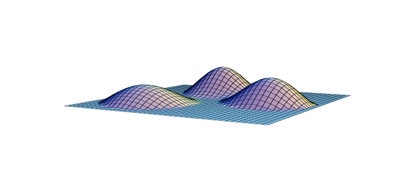
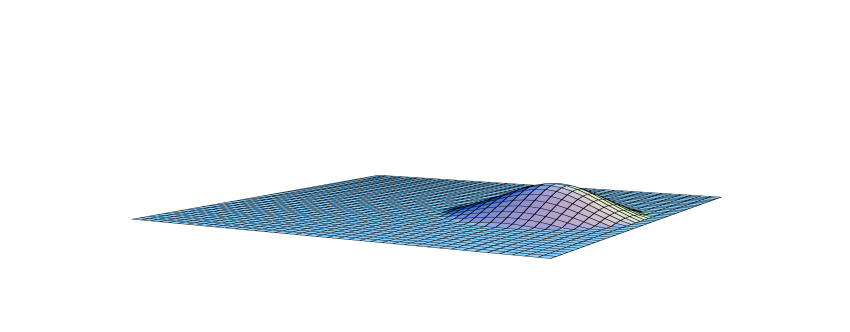
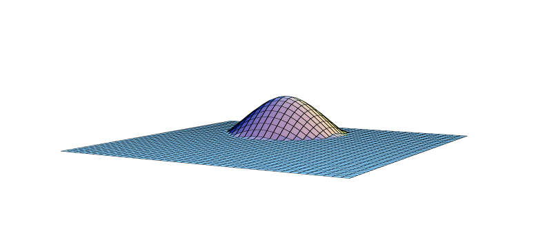
Figure 1: The action densities (top) for the $SU(3)$ caloron, cut off at $1/(2e)$, on a logarithmic scale, with $(\mu_{1},\mu_{2},\mu_{3})=(-17,-2,19)/60$ for $t\!=\!0$ in the plane defined by $\vec{y}_{1}\!=\!(-2,-2,0)$, $\vec{y}_{2}=(0,2,0)$ and $\vec{y}_{3}=(2,-1,0)$, for ${\beta}=1$, with masses $8\pi^{2}\nu_{i}$, $(\nu_{1},\nu_{2},\nu_{3})=(0.25,0.35,0.4)$. On the bottom-left is shown the zero-mode density for fermions with anti-periodic boundary conditions in time and on the bottom-right for periodic boundary conditions, at equal logarithmic scales, cut off below $1/e^{5}$.

This localisation can be established easily in the limit of large $|\vec{y}_{i}\!\!-\!\vec{y}_{i+1}|$ for all $i$, in which case one finds, when $z\in[\mu_{m},\mu_{m+1}]$,

$$\!\hat{f}_{x}(z,z)\!\!=\!\!\frac{\sinh[2\pi(z\!-\!\mu_{m})r_{m}]\sinh[2\pi(\mu_{m+1}\!-\!z)r_{m}]}{r_{m}\sinh[2\pi\nu_{m}r_{m}]/2\pi}\hskip-22.76219pt$$

making explicit that the location of the zero-mode is determined by the interval that contains the appropriate value of $z$. From eq. (2) it follows that $\mu_{1}\!\leq\!0\!\leq\!\mu_{n}$, such that the periodic zero-mode is associated to the static constituent at $\vec{y}_{m}$, with $\mu_{m}\!\leq\!0\!\leq\!\mu_{m\!+\!1}$. This is precisely the condition for the existence of a zero-mode given by the Callias index theorem [10] (see also the appendix of ref. [11]). Due to the static background (for well-separated constituents), time dependence of the zero-mode would be of the form $\exp(2\pi ikt)$ for $k$ integer, shifting $z\!=\!0$ by $k$, out of the interval that allows for a zero-mode.

Allowing for $k\!=\!\pm{\scriptstyle{{1\over 2}}}$, for which $\exp(2\pi ikt)$ turns the periodic zero-mode anti-periodic, we can have situations where this anti-periodic zero-mode is associated to one of the static monopole constituents. A specific example for $SU(3)$ where this occurs is $(\mu_{1},\mu_{2},\mu_{3})\!=\!(-0.48,-0.03,0.51)$, yielding $(\nu_{1},\nu_{2},\nu_{3})\!=\!(0.45,0.54,0.01)$. Both the periodic and the anti-periodic zero-mode are associated to the $2^{\rm nd}$ constituent. We note that, apart from the fact that the $3^{\rm rd}$ constituent is nearly massless, both zero-modes are very broad since min$(z\!-\!\mu_{2},\mu_{3}\!-\!z)\!=\!0.03$ for $z\!=\!0$ and $0.01$ for $z\!=\!{\scriptstyle{{1\over 2}}}$. For $SU(2)$ $z\!=\!0$ is always midway between $\mu_{1}$ and $\mu_{2}$ and $z\!=\!{\scriptstyle{{1\over 2}}}$ midway between $\mu_{2}$ and $\mu_{3}\!=\!1\!+\!\mu_{1}$). When $z$ coincides with $\mu_{i}$, the zero-mode is no longer normalisable, which is the origin of the delta function singularities in the Nahm transformation.

4 Conclusions

In conclusion, for well-separated constituents the fermion zero-mode is localised to a single constituent. For $SU(2)$ the anti-periodic zero-mode is always associated to the constituent that carries Taubes-winding [9]. For $SU(n\!>\!2)$ this is also typically true (see fig. 1), in particular when well localised, something that may be significant for developing a model for the QCD vacuum that combines monopoles and instantons [2, 3, 9]. However, exceptions exist where both the periodic and anti-periodic zero-mode are associated to (possibly the same) static constituent(s), although this tends to be accompanied by nearly massless constituents, and rather delocalised zero-modes.

References

• [1] T.C. Kraan and P. van Baal, Phys. Lett. B435 (1998) 389.
• [2] T.C. Kraan and P. van Baal, Nucl. Phys. B(Proc.Suppl.) 73 (1999) 554.
• [3] T.C. Kraan and P. van Baal, Phys. Lett. B428 (1998) 268; Nucl. Phys. B533 (1998) 627.
• [4] W. Nahm, Self-dual monopoles and calorons, in: Lecture Notes in Physics 201 (1984) 189.
• [5] M.F. Atiyah, N.J. Hitchin, V. Drinfeld and Yu.I. Manin, Phys. Lett. 65A (1978) 185
• [6] K.Lee and P. Yi, Phys. Rev. D56(1997)3711; K.Lee and C.Lu, Phys.Rev.D58(1998)025011.
• [7] C. Taubes, in: Progress in gauge field theory, eds. G.’t Hooft e.a., (Plenum Press, New York, 1984) p.563
• [8] N.M. Davies, T.J. Hollowood, V.V. Khoze and M.P. Mattis, hep-th/9905015.
• [9] M.GarcΓ­aΒ PΓ©rez, A.GonzΓ‘lez-Arroyo, C.Pena and P. van Baal, Phys.Rev. D60(1999)031901.
• [10] C.J. Callias, Comm.Math.Phys. 62(1978)213.
• [11] J. de Boer, K. Hori and Y. Oz, Nucl. Phys. B500 (1997) 163.