Ergodic Properties of Classical SU(2) Lattice Gauge Theory

Abstract

We investigate the relationship between the Lyapunov exponents of periodic trajectories, the average and fluctuations of Lyapunov exponents of ergodic trajectories, and the ergodic autocorrelation time for the two-dimensional hyperbola billiard. We then study the fluctuation properties of the ergodic Lyapunov spectrum of classical SU(2) gauge theory on a lattice. Our results are consistent with the notion that this system is globally hyperbolic. Among the many powerful theorems applicable to such systems, we discuss one relating to the fluctuations in the entropy growth rate.

I Introduction

Extensive experimental efforts are under way at Brookhaven National Laboratory and CERN to produce and investigate the new deconfined, chirally symmetric high-temperature phase of QCD, usually called the quark-gluon-plasma (QGP). While the very high energy densities generated in high-energy nuclear collisions virtually guarantee that some new state of matter is reached, there are still important unresolved theoretical problems relating to the description of this state. One missing, critical ingredient is a non-perturbative approach to dynamical QCD processes far from thermodynamical equilibrium.

The study of non-equilibrium dynamics of relativistic quantum fields is currently an active area of theoretical research [2]. Approaches that go beyond perturbation theory include descriptions in terms of probabilistic transport equations [3], and deterministic or stochastic classical equations for the infrared degrees of freedom of the quantum fields [4, 5]. In the special, but important case of non-Abelian gauge theories, the extreme infrared limit has been long known to correspond to a dynamical system exhibiting classical as well as quantum chaos [6, 7]. Several years ago, this result was extended to spatially varying, lattice regulated Yang-Mills fields by numerical calculation of the maximal Lyapunov exponents and the complete ergodic Lyapunov spectrum of classical SU(2) gauge theory [8, 9, 10]. The most intriguing results with implications for relativistic heavy ion physics are:

1. The ergodic Lyapunov spectrum looks exactly as expected for a globally hyperbolic system.

2. The largest Lyapunov exponent appears to be related to the plasmon damping rate as predicted by high temperature perturbation theory [11].

3. The magnitude of the maximal Lyapunov exponent for SU(3) indicates a rapid thermalization of gluons in heavy-ion collisions.

These results suggest the extension of this approach to a systematic semi-classical description of the dynamics of Yang-Mills field theories. The success of such an approach will ultimately depend on one’s ability to find practical methods for the application of periodic orbit theory to systems with many degrees of freedom. We discuss a very first step in this direction.

We present results of an investigation of the relation between the Lyapunov exponents of periodic and ergodic orbits. Periodic orbit theory, in the framework of the thermodynamic formalism, makes detailed predictions for the statistical properties of Lyapunov exponents of generic orbits in Anosov systems, but few studies of these relations appear to have been made for specific chaotic, non-linear dynamical systems. This motivated our numerical study of the relation between the Lyapunov exponents of periodic orbits and generic trajectories in a system for which the Lyapunov exponents of periodic orbits (henceforth simply called “periodic Lyapunov exponents”) are known for all orbits below a certain period: the two-dimensional hyperbola billiard [12]. For this system, therefore, powerful mean value theorems can be invoked to predict analytical relations which can be checked numerically. Below, we present our numerical results confirming the general connection between the Lyapunov exponents for ergodic and periodic orbits as well as for their fluctuations.

We then dicuss the corresponding properties of the Lyapunov exponents of ergodic trajectories for classical SU(2) Yang-Mills theory on a three-dimensional lattice. The observed similarities suggest that this system is also globally hyperbolic and could, in principle, be treated within the framework of periodic orbit theory. Our conjecture yields a prediction for the fluctuation properties of the ergodic Lyapunov exponents which is verified numerically. On the basis of the relation between these fluctuations and the fluctuations of the entropy growth rate we obtain a prediction of the magnitude of entropy fluctuations as a function of space-time volume. We find that for the conditions occurring in high energy nuclear collisions these fluctuations are expected to be very small, in agreement with observations.

We emphasize that it is presently impossible to predict how far this approach will carry toward a description of the dynamics of non-equilibrium processes in QCD. Classical Yang-Mills equations can only be used to estimate a very limited number of dynamical parameters of the QGP, namely those which have a well-defined classical limit, such as the logarithmic entropy growth rate, $d(\ln S)/dt$, but not quantities such as the energy or entropy density. Our analysis is only relevant to the fluctuation properties of such, essentially “classical” quantities. However, we hasten to point out that, independently of the specific application considered here, an improved understanding of the connection between quantum field theory and periodic orbit theory is of fundamental theoretical relevance for non-linear dynamics in general. To our knowledge for the first time, we propose a general relationship between the mean periodic Lyapunov exponents of a dynamical system, its mean ergodic Lyapunov exponents, and the ergodic autocorrelation time. This general relationship makes it possible to extract important new information for any higher-dimensional system for which the explicit construction of the periodic orbits is practically not feasible.

The basic assumption underlying periodic orbit theory is that the periodic orbits sample the phase space of a non-linear dynamical system in such a manner that its averaged properties can be systematically reconstructed from the properties of the periodic orbits. For each such orbit there is a spectrum of characteristic Lyapunov exponents that describe how fast the separation between neighboring orbits increases with time. While periodic orbit theory is an extremely powerful tool, its range of applicability is strongly limited by the difficulties encountered in determining the complete set of periodic orbits. For any field theory with its potentially infinitely many degrees of freedom, the task of numerically constructing the periodic orbits looks hopeless. It is, however, relatively easy to obtain ergodic Lyapunov exponents by numerical integration of the equations of motion [8]. Since it seems plausible that every ergodic trajectory eventually comes close to any periodic orbit, any infinite ergodic orbit should sample all periodic orbits. Thus it appears as a natural conjecture that the average properties of ergodic Lyapunov exponents and the average properties of periodic Lyapunov exponents should be related. It is this relationship that we want to discuss in the following.

II General Relations

Before we investigate and confirm the relationship between ergodic and periodic orbits for a simple but non-trivial system for which all periodic Lyapunov exponents (up to a certain period) are known, namely, the two-dimensional hyperbola billiard [12], we review some general relations between Lyapunov exponents of periodic and generic trajectories. In the next section, we will compare these analytic predictions for the properties of the ergodic Lyapunov exponents $\lambda_{\rm r}$ with those obtained by numerical integration of a randomly chosen ergodic trajectory $\vec{x}(t)=\vec{x}_{0}(t)+\delta\vec{x}(t)$:

$$\lambda_{\rm r}=\lim_{\delta\vec{x}(0)\rightarrow 0}\lim_{t\rightarrow\infty}{1\over t}\ln{|\delta\vec{x}(t)|\over|\delta\vec{x}(0)|}\ ,$$ (1)

where the index $r$ indicates the random starting point. (We remind the reader that for a fully ergodic system this yields the maximal ergodic Lyapunov exponent, which for $d=2$ degrees of freedom is the unique positive exponent.)

In a Hamiltonian hyperbolic dynamical system with $d$ degrees of freedom ergodicity implies that the sum of its $d-1$ positive ergodic Lyapunov exponents can also be obtained as the ergodic mean of the local expansion rate,

$$\lim_{t\rightarrow\infty}h_{\rm r}(t)\equiv\lim_{t\rightarrow\infty}{1\over t}\int_{0}^{t}\chi(\vec{x}(t^{\prime}))\ dt^{\prime}=\sum_{j=1}^{d-1}\lambda_{r,j}=h_{\rm KS}\ .$$ (2)

Here $h_{\rm KS}$ denotes the Kolomogorov-Sinai entropy and

$$\chi(\vec{x}(t))={d\over dt}\ln\det\left({\partial\vec{x}(t)\over\partial\vec{x}(0)}\right)_{\rm expanding}$$ (3)

is the local rate of expansion along the trajectory $\vec{x}(t)$. Due to the equidistribution of periodic orbits in phase space it is possible to evaluate the ergodic mean in (2) by weighted sums over periodic orbits. In fact, for hyperbolic systems the thermodynamic formalism allows to express certain invariant measures on phase space in terms of averages over periodic orbits, see, e.g., [13, 14]. One is in particular able to obtain a relation that establishes a direct connection between the positive ergodic Lyapunov exponents $\lambda_{r,j}$ and those of periodic orbits. Labelling periodic orbits by $\nu$, and denoting their periods and positive Lyapunov exponents by $T_{\nu}$ and $\lambda_{\nu,j}$, respectively, this relation reads

$$\sum_{j=1}^{d-1}\lambda_{r,j}=\lim_{t\rightarrow\infty}\frac{\sum_{t\leq T_{\nu}\leq t+\varepsilon}\left(\sum_{j=1}^{d-1}\lambda_{\nu,j}\right)\exp\left(-\sum_{j=1}^{d-1}\lambda_{\nu,j}T_{\nu}\right)}{\sum_{t\leq T_{\nu}\leq t+\varepsilon}\exp\left(-\sum_{j=1}^{d-1}\lambda_{\nu,j}T_{\nu}\right)}\ ,$$ (4)

where $\varepsilon>0$ is arbitrary. Within the thermodynamic formalism the topological pressure $P(\beta)$ was introduced as a useful tool to analyze invariant measures on phase space in terms of periodic orbits as, e.g., in (4). This function can be expressed as

$$P(\beta)=\lim_{t\rightarrow\infty}{1\over t}\ln\sum_{t\leq T_{\nu}\leq t+\varepsilon}\exp\left(-\beta\sum_{j=1}^{d-1}\lambda_{\nu,j}T_{\nu}\right)\ ,$$ (5)

and it is not difficult to derive from (5) that $P(\beta)$ is monotonically decreasing and convex. The exponential proliferation of the number of periodic orbits immediately implies that $P(0)=h_{top}$ (topological entropy). Moreover, the arithmetic average of the sum of the positive periodic Lyapunov exponents is given by $\bar{\lambda}=-P^{\prime}(0)$. The relation (4) then follows from (2) and from the non-trivial identity $-P^{\prime}(1)=h_{\rm KS}$. One also concludes that the three quantities measuring a mean separation of neighboring trajectories are ordered in the following way: $\bar{\lambda}\geq h_{top}\geq h_{\rm KS}$. For further information see, e.g., [14].

Our next goal is to investigate the fluctuations of the local rate of expansion (3), when integrated up to a sampling time $t_{\rm s}$, about its ergodic mean (2). We recall that this quantity was denoted as $h_{\rm r}(t_{\rm s})$ in (2). For (uniformly) hyperbolic dynamical systems one expects that observables sampled along ergodic trajectories up to time $t_{\rm s}$ show Gaussian fluctuations about their ergodic mean. Indeed, in many cases a central limit theorem holds true that also predicts the widths of these Gaussian to scale as $t_{\rm s}^{-1/2}$ for large sampling times $t_{\rm s}$. More precisely, Waddington [15] has shown that for Anosov systems (i.e., fully hyperbolic systems on compact phase spaces) the difference

$$\sqrt{t_{\rm s}}\left[h_{\rm r}(t_{\rm s})-h_{\rm KS}\right]$$ (6)

shows Gaussian fluctuations with variance $P^{\prime\prime}(1)$ in the limit $t_{\rm s}\rightarrow\infty$. This means that

$$\Delta h_{\rm r}(t_{\rm s})\sim\sqrt{P^{\prime\prime}(1)/t_{\rm s}}\ ,\quad t_{\rm s}\rightarrow\infty\ .$$ (7)

According to (5) the quantity $P^{\prime\prime}(1)$ can be expressed in terms of periodic orbit sums as

$$P^{\prime\prime}(1)=\lim_{t\to\infty}t\left[\frac{\sum_{\nu}\left(\sum_{j}\lambda_{\nu,j}\right)^{2}\exp\left(-\sum_{j}\lambda_{\nu,j}T_{\nu}\right)}{\sum_{\nu}\exp\left(-\sum_{j}\lambda_{\nu,j}T_{\nu}\right)}-\left(\frac{\sum_{\nu}\left(\sum_{j}\lambda_{\nu,j}\right)\exp\left(-\sum_{j}\lambda_{\nu,j}T_{\nu}\right)}{\sum_{\nu}\exp\left(-\sum_{j}\lambda_{\nu,j}T_{\nu}\right)}\right)^{2}\right]\ .$$ (8)

On the other hand, the variance of the distribution of the periodic Lyapunov exponents is related to $P^{\prime\prime}(0)$, since

$$P^{\prime\prime}(0)=\lim_{t\to\infty}t\left[\frac{\sum_{t\leq T_{\nu}\leq t+\varepsilon}\left(\sum_{j=1}^{d-1}\lambda_{\nu,j}\right)^{2}}{\sum_{t\leq T_{\nu}\leq t+\varepsilon}1}-\left(\frac{\sum_{t\leq T_{\nu}\leq t+\varepsilon}\left(\sum_{j=1}^{d-1}\lambda_{\nu,j}\right)}{\sum_{t\leq T_{\nu}\leq t+\varepsilon}1}\right)^{2}\right]\ .$$ (9)

For the hyperbola billiard this variance was calculated numerically by Sieber [12], who found Gaussian distributions of the positive Lyapunov exponents of periodic orbits with $N$ bounces off the boundary. For large $N$ the widths of these Gaussian scale like

$$\tilde{\sigma}_{N}\sim{0.199\over\sqrt{N}}\ .$$ (10)

Taking into account that the mean length of periodic orbits with $N$ bounces scales as $\bar{t}_{N}\sim 2.027N$ [12], this yields a prediction for the width of the distribution of periodic Lyapunov exponents expressed as a function of $t$ that scales as

$$\Delta\lambda_{\nu}(t)\sim{0.283\over\sqrt{t}}$$ (11)

in the limit of long periodic orbits. One hence concludes that $P^{\prime\prime}(0)=0.08$.

The variance of the fluctuations (6) can also be related to the autocorrelation function

$$a(\tau)=\langle\chi(\vec{x}(\tau))\,\chi(\vec{x}(0))\rangle-(h_{\rm KS})^{2}$$ (12)

of the local ergodic Lyapunov exponents, where $\langle\dots\rangle$ denotes a phase space average. In order to derive this connection one averages the square of (6) over phase space, which then leads to

$$t\,(\Delta h_{\rm r}(t))^{2}={1\over t}\int_{-t}^{+t}(t-|\tau|)\,a(\tau)\ d\tau\ .$$ (13)

A connection with the topological pressure can be established because (6) and (7) imply that the autocorrelation function (12) vanishes faster than $1/\tau$ as $\tau\to\infty$. One can therefore perform the limit $t\to\infty$ on both sides of (13), yielding

$$P^{\prime\prime}(1)=\lim_{t\rightarrow\infty}t\,(\Delta h_{\rm r}(t))^{2}=\int_{-\infty}^{+\infty}a(\tau)\ d\tau\ .$$ (14)

Finally we want to discuss the probability for deviations of the sum of the positive ergodic Lyapunov exponents, sampled over time $t$, from its ergodic mean $h_{\rm KS}$. To this end let $p_{t}(h)$ denote the probability density for $h_{\rm r}(t)$ to have a value $h$. Waddington has shown [15] that for Anosov systems which are such that $P^{\prime\prime}(\beta)\neq 0$ for all $\beta$, this probability density has the form

$$p_{t}(h)=f(h)\,\sqrt{t}\,\exp(-g(h)t)\ ,$$ (15)

where $f(h)$ is a complicated, though uniquely fixed function. Moreover,

$$g(h)=\inf_{\beta}\{h\beta+P(\beta+1)\}$$ (16)

is a strictly convex, non-negative function with a unique minimum at the ergodic mean $h_{min}=h_{\rm KS}$, where $g(h_{\rm KS})=0$. This means that for large $t$ the probability of large deviations of $h_{\rm r}(t)$ from the ergodic mean is exponentially small.

III The Two-Dimensional Hyperbola Billiard

We test the above statements in the two-dimensional hyperbola billiard, for which all periodic orbits and their Lyapunov exponents are known up to certain orbit period [12]. In order to be able to compare our numerical results with the analytical predictions, which are based on periodic orbits in a restricted length range, we have limited the motion into the arms of the hyperbola billiard, using the cut-off $|x|,|y|\leq x_{\rm lim}=10/\sqrt{2}$ and reflecting the motion horizontally or vertically at the boundary. We have not studied the dependence of our results on $x_{\rm lim}$ in any systematic fashion, but a cursory exploration did not reveal a significant dependence.

Our numerical result for the KS-entropy was obtained as $h_{\rm KS}\equiv\lambda_{\rm r}=0.575$ by exploiting the relation (1) for the positive ergodic Lyapunov exponent. In [12] the arithmetic average of the periodic Lyapunov exponents and the topological entropy have been determined numerically as $\bar{\lambda}=0.703$ and $h_{\rm top}=0.5925$, respectively, so that the ordering $\bar{\lambda}\geq h_{\rm top}\geq h_{\rm KS}$ is respected. This provides a non-trivial test since the general theoretical statement has only been proven for uniformly hyperbolic systems (Anosov systems) on compact phase spaces. The hyperbola billiard is only non-uniformly hyperbolic and, moreover, without the imposed cut-off its phase space fails to be compact.

For the (cut-off) hyperbola billiard we found that the distributions of the ergodic Lyapunov exponents (1) that we determined numerically up to sampling times $t_{\rm s}$ are very well described by Gaussians, see Fig. 1, if the sampling time is not too small ($t_{\rm s}\gg 1$). For small sampling times, most of the phase space divergence occurs during intervals $t_{\rm s}$ when the trajectory reflects off the hyperbolic boundary, making the distribution of $h_{\rm r}(t_{\rm s})\equiv\lambda_{\rm r}(t_{\rm s})$ strongly non-Gaussian in the limit $t_{\rm s}\to 0$. We made power-law fits of the form $at_{\rm s}^{-b}$ to the dependence of the widths of these Gaussians on $t_{\rm s}$. This gave the result (see Fig. 2):

$$\Delta h_{\rm r}(t_{\rm s})\approx 0.86\,t_{\rm s}^{-1/2}\ .$$ (17)

We also determined the correlation function $a(\tau)$ for the hyperbola billiard by sampling $h_{\rm r}(t_{\rm s})$ for in small intervals $t_{\rm s}=1/(2\sqrt{2})$. The result is shown in Fig. 3. Clearly, $a(\tau)$ falls off rapidly with a time constant of about $t_{c}=6$. Therefore, we can test the relation (13) by integrating the right-hand side numerically. For $t=28.3$, corresponding to the lower plot in Fig. 1, we obtain in this way the prediction $\Delta h_{\rm r}=0.197$ with an estimated numerical uncertainty of about 25%. The value obtained from the Gaussian fit to the histogram in Fig. 1 is $\Delta h_{\rm r}=0.159$. The quality of this agreement must be judged with the fact in mind that the correlation function $a(\tau)$, as well as the distribution $\chi(\vec{x}(t))$ are highly singular for the hyperbola billiard in the limit $\tau\to 0$.

IV The SU(2) gauge theory on a lattice

Let us now turn to a comparison with results obtained for ergodic orbits in the classical SU(2) Yang-Mills theory regularized on a lattice. In [10] the complete (positive) Lyapunov spectra were obtained for lattice volumes $L^{3}$ with $L=1,2,3$. We have extended these calculations to the lattices of size $L=4,6$. All our calculations were performed for an average energy per plaquette $E_{\rm p}\approx 1.8$. For sufficiently long trajectories and fixed energy per lattice site the Lyapunov spectrum has a unique shape, independent of the lattize size, as shown in Fig.5. Indeed, for a completely hyperbolic system, physical intuition requires that the Kolmogorov-Sinai entropy $-P^{\prime}(1)$ is an extensive quantity. For this to be true, the sum over all positive Lyapunov exponents must scale like the lattice volume $L^{3}$ and the shape of the distribution of Lyapunov exponents must be independent of $L$. Figure 5 confirms this expectation.

In Fig. 6 we show distributions of the sum over positive Lyapunov exponents as a function of the length of the sampled ergodic trajectories (obtained as function of the sampling time $t_{\rm s}$ on a single, very long trajectory). Obviously, the distributions are nicely fitted by Gaussians whose widths decrease like $1/\sqrt{t_{\rm s}}$ (see Fig. 7). This behavior is identical to that of the two-dimensional hyperbolic system studied before (cf. Fig. 1). We also determined again the autocorrelation function $a(\tau)$ defined in (12) by sampling the distribution $p_{t}(h)$ with small time steps (see top part of Fig. 4). For the $L=4$ lattice the result is shown in the lower part of Fig. 4. This allows us to test the relation (13) connecting the $a(\tau)$ with the variance of the ergodic Lyapunov exponents. Using (13) we obtain the value $\Delta h_{\rm r}=0.88$ for $t_{\rm s}=6$, whereas the Gaussian fit to the sampled distribution shown in the top part of Fig. 6 is $\Delta h_{\rm r}=0.83$.

One can also read off from the distributions shown in Fig. 6 how the widths of the Gaussians scale with the lattice size $L$. To a very good approximation we find that it is proportional to $\sqrt{L^{3}}$. If one includes the sampling time dependence, the variance of $h_{\rm KS}$ scales like $\sqrt{L^{3}/t_{\rm s}}$. As the mean value $h_{\rm KS}$ of the distribution $p_{t}(h)$ scales like $L^{3}$, this result confirms the Gaussian nature of the fluctuations. Our result also has important consequences for heavy-ion collisions. If fluctuations are Gaussian with a dimensional scale given by the mean maximal ergodic Lyapunov exponent, which is found numerically to be of order (0.5 fm)^-1 [8], then for typical volumes and reaction times encountered in nuclear reactions the relative fluctuations must be very small, of order $\sqrt{(0.5\,{\rm fm})^{4}/(5\,{\rm fm})^{4}}=0.01$. This result is in agreement with a recent measurement of the fluctuations in relativistic heavy-ion collisions, which show that the primary event-by-event fluctuations in the mean value of the transverse momentum do not exceed 1 percent [16].

Let us stress that while it is consistent to assume that the SU(2) gauge theory treated as a classical field theory on the lattice is a hyperbolic system, our positive evidence is limited. It should be clear that it is impossible to exclude, by numerical calculations for a limited number of trajectories, that there are regions in the high-dimensional phase space of our lattice field theory which are not hyperbolic. (Then the SU(2) field on the lattice would not be an Anosov system.) Also it is unproven, though highly probable, that the addition of the quarks will not change the picture.

V Conclusions

We have shown by numerical simulations that for a two-dimensional billiard the mean values for the ergodic and periodic Lyapunov exponents and their fluctuations as a function of trajectory length (i.e. time) are closely related. We have derived a general relation between their mean values and checked it numerically. This demonstrates that we understand the relationship between ergodic and periodic Lyapunov exponents for the hyperbola billiard. We have than analyzed in a similar way classical SU(2) gauge theory on a lattice. For all investigated properties we found good agreement with the expectations for a globally hyperbolic (Anosov) system. We conclude that for all quantities of interest which have a well-defined classical limit (like the growth rate of entropy after the initial energy deposition by hard interactions) the probability for large fluctuations should be exponentially small. For typical high-energy heavy-ion collisions (Pb+Pb) such fluctuations are estimated to be at most of the order of a few percent.

FIG. 1.: Distribution the calculated local Lyapunov exponents for ergodic trajectories of two different length $t_{\rm s}$ in the hyperbola billiard.

FIG. 2.: The widths of the Gaussians illustrated in Fig. 1 as a function of $t_{\rm s}$ together with a fits of the form $at_{\rm s}^{-1/2}$ (solid line) and $at_{\rm s}^{-b}$ with $b=0.45$ (dashed line).

FIG. 3.: Temporal autocorrelation for the local Lyapunov exponents determined along an ergodic trajectory in the two-dimensional hyperbola billiard. The dashed line is a fit of the form $a\exp(-\tau^{2}/t_{c}^{2})$ yielding $t_{c}\approx 6$.

FIG. 4.: Distribution of numerically obtained ergodic Lyapunov exponents for a classical SU(2) gauge theory on lattices of size $L=2,4,6$. The index $i$ numbers the Lyapunov exponents and the abscissa is scaled with $L^{3}$.

FIG. 5.: Distributions of the sum of the positive ergodic Lyapunov exponents for different values of the trajectory length $t_{\rm s}$ for classical lattice SU(2) gauge theory on lattices of size $L=4,6$.

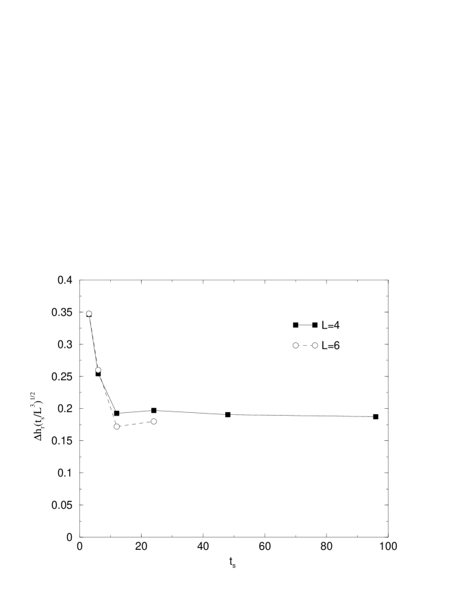
FIG. 6.: The widths of the Gaussians illustrated in Fig. 5 and scaled with $(t_{\rm s}/L^{3})^{1/2}$, as a function of $t_{\rm s}$.

FIG. 7.: Top: The distribution of the sum of local expansion rates $h_{\rm r}$ for L=4 and a short sampling time $t_{\rm s}=0.1$, together with a Gaussian fit. Because the globally expanding phase space volume may be locally contracting, the distribution has a small tail extending to negative values of $h_{\rm r}$. This tail disappears (becomes exponentially small) for large values of $t_{\rm s}$. Bottom: The autocorrelation function $a(\tau)$ for this distribution.

REFERENCES

- [1]
- [2] D. Boyanovsky, H.J. de Vega, R. Holman, S. Prem Kumar, R.D. Pisarski, and J. Salgado, preprint hep-ph/9810209; C. Wetterich, Phys. Rev. E 56, 2687 (1997); F. Cooper, S. Habib, Y. Kluger, E. Mottola, J.P. Paz, and P.R. Anderson, Phys. Rev. D 50, 2848 (1994); E. Calzetta and B.L. Hu, Phys. Rev. D 37, 2878 (1988).
- [3] H.T. Elze and U. Heinz, Phys. Rept. 183, 81 (1989); P.F. Kelly, Q. Liu, C. Lucchesi, and C. Manuel, Phys. Rev. D 50, 4209 (1994).
- [4] M. Gleiser and R.O. Ramos, Phys. Rev. D 50, 2441 (1994); C. Greiner and B. Müller, Phys. Rev. D 55, 1026 (1997).
- [5] D. Bödeker, Phys. Lett. B 426, 351 (1999) and preprint hep-ph/9905239; P. Arnold, D.T. Son, and L.G. Yaffe, Phys. Rev. D 59, 105020 (1999).
- [6] S.G. Matinyan, G.K. Savvidy, and N.G. Ter-Arutunian Savvidy, JETP Lett. 53, 421 (1981) [Pis’ma Zh. Eksp. Teor. Fiz. 34, 613 (1981)].
- [7] G.K. Savvidy, Nucl. Phys. B 246, 302 (1984).
- [8] B. Müller and A. Trayanov, Phys. Rev. Lett. 68, 3387 (1992); T.S. Biró, C. Gong, B. Müller, and A. Trayanov, Int. J. Mod. Phys. C 5, 113 (1994).
- [9] C. Gong, Phys. Lett. B 298, 257 (1993).
- [10] C. Gong, Phys. Rev. D 49, 2642 (1994).
- [11] T.S. Biró, C. Gong, and B. Müller, Phys. Rev. D 52, 1260 (1995).
- [12] M. Sieber, The Hyperbola Billiard: A Model for the Semiclassical Quantization of Chaotic Systems, DESY preprint 91-030; M. Sieber and F. Steiner, Physica D 44, 248 (1990).
- [13] W. Parry and M. Pollicott, Zeta Functions and the Periodic Orbit Structure of Hyperbolic Dynamics, Astérisque 187-188 (1990).
- [14] P. Gaspard, Chaos, Scattering and Statistical Mechanics, Cambridge University Press (1998).
- [15] S. Waddington, Ann. Inst. Henri Poincaré C 13, 445 (1996).
- [16] H. Appelshäuser et al. (NA49 collaboration), preprint hep-ex/9904014.