Stochastic Estimator Techniques and Their Implementation on Distributed Parallel Computers

Abstract

The calculation of physical quantities by lattice QCD simulations requires in some important cases the determination of the inverse of a very large matrix. In this article we describe how stochastic estimator methods can be applied to this problem, and how such techniques can be efficiently implemented on parallel computers.

WUB-99-16

1 Introduction

Within our current level of comprehension of the fundamental principles of nature, physical processes on an atomic or subatomic scale can be successfully described by Quantum Field Theories (QFT). In such theories particles as well as their interactions are represented by quantum fields, defined at each space-time point. The value of a physical quantity, which can be measured in experiment, can be calculated by a weighted average over all “would be” values of this quantity, achieved for each possible configuration of the quantum fields involved. The weight with which each of these “would be” values contributes is determined by the so called action, a scalar quantity which contains the characteristic features of the QFT in question and which depends on the quantum fields. The formal expression of this averaging procedure is known as the path functional.

An exact analytical treatment of the path functional is in most cases not possible. Approximate solutions can be achieved in the framework of perturbation theory if the interaction strength is weak. Perturbative methods have been proven very successful in the evaluation of the QFT of the electromagnetic and weak forces. They fail however when applied to the QFT of the strong force, the so called Quantum Chromo Dynamics (QCD). The strong force is responsible for a large range of phenomena at and below the scale of the atomic nuclei.

Lattice QCD is designed for a non-perturbative numerical evaluation of QCD. The space-time continuum is approximated by a lattice with $N_{s}^{3}\times N_{t}$ space-time points. The calculation of physical quantities is done in two steps. First, one generates a representative sample of quantum field configurations, where each configuration is represented according to its specific weight, by a Monte Carlo procedure mc_quenched ; mc_full ; Kennedy_here . Secondly, one determines the “would be” value of the physical quantity in question on each of the quantum field configurations and takes the average. We call the latter step the analysis of quantum field configurations.

Clearly, the computational effort which has to be invested in the analysis part depends on the physical quantity one is interested in. In this article we report on a computationally very hard problem which occurs in the analysis of configurations with respect to so called disconnected contributions. The latter are of great physical importance as they are expected to play a substantial role in the solution of the “proton spin problem” review_ga and of the “$U(1)$ problem” of QCD reviews_u1 .

Naively, the calculation of disconnected contributions requires the inversion of a complex matrix of size $(N_{s}^{3}\times N_{t}\times 12)^{2}$ on each single quantum field configuration. For currently available lattice sizes, see ref.burkhalter , such a calculation would be prohibitively expensive. To circumvent this problem one applies stochastic estimator methods which converge to the true result in the stochastic limit. It turns out however, that even with such techniques one still needs a parallel supercomputer to handle this problem.

This article is organized as follows. In the next section we will give an impression of the physical meaning of disconnected contributions. Section 3 explains what has to be done technically to calculate such contributions. Section 4 is devoted to the stochastic estimator techniques. The implementation of these techniques on parallel computers is discussed in section 5. Section 6 will give an overview of state of the art calculations of disconnected contributions. Section 7 contains a short summary.

2 The Physical Motivation

It is nicely explained by R. Gupta in this volume gupta_here that our “parton” picture of a proton as being made of 3 interacting quarks is not applicable in full QCD. The reason is that in this case the spontaneous creation and annihilation of quark antiquark pairs leads to an additional contribution to the proton amplitude. This is shown in Gupta’s fig.3.

Suppose that we would like to investigate the properties of a proton by a scattering experiment, e.g. by deep inelastic $\mu$p (muon proton) scattering. Then, the $\mu$p scattering amplitudes measured in such an experiment could in principle differ sizably from the parton expectation since the latter neglects the interaction of the $\mu$ particle with the quark antiquark loop.

To illustrate this point we show in fig. 1 the full QCD contributions to the propagator of a proton which interacts with an external current $j$.

Figure 1: Connected (a) and disconnected (b) contributions to a proton interacting with a current $j$. All quark lines, including the quark loop, are connected by infinitely many gluon lines and virtual quark loops.

Part (a) of the figure depicts the naive (parton) case, where the current couples to one of the quarks of the proton. Part (b) shows the interaction of the current $j$ with a quark antiquark loop, in the field of the proton. This disconnected contribution is present only in full QCD. We emphasize that the location in space and time of the quark antiquark loop is not fixed. Thus, to calculate the disconnected contribution one has to sum over all positions.

Of course, it is not obvious from these considerations that the disconnected part really gives non negligible contributions to the scattering amplitudes. In fact, it turns out that many of them have a structure such that their net contribution is expected to be small.

There is however a class of amplitudes, the flavor singlet amplitudes, where disconnected contributions can be sizeable. In order to investigate quark loop effects in QCD it is therefore of utmost interest to calculate flavor singlet amplitudes and to compare the results with experimentally measured data.

From experimental measurements one can extract the values of at least 2 flavor singlet amplitudes. The first, which describes the interaction of a proton with a pseudo-vector current deviates by about a factor of 2 from the naively expected value. This deviation gave rise to the so called “proton spin crisis”. The second, which couples a scalar current to a proton, yields, when multiplied by the quark mass, the pion-nucleon sigma term $\Sigma_{\pi N}$ gasser_nsigma . The experimental value of this quantity also differs by about a factor of 2 from the naive expectation. Thus, these quantities are most promising candidates to study the influence of quark loops by a full QCD lattice simulation.

Disconnected amplitudes are supposed to contribute also to many physical processes other than proton scattering. For example, a (pseudo scalar) meson, which is made of a quark and an antiquark, can be “mimicked”, with respect to its quantum numbers, by 2 quark antiquark loops. This is shown in fig.2.

Figure 2: Connected (a) and disconnected (b) contributions to the propagator of a pseudo scalar meson.

An experimental measurement of e.g. the mass of this meson would include both terms, connected and disconnected.

From symmetry considerations one again concludes, that the disconnected part should contribute mostly if the quarks in the meson are put together in a flavor singlet combination. Experimentally, one finds that the mass of such a flavor singlet meson, which is named $\eta^{\prime}$, is much larger than that of its non-singlet partners. This discrepancy is called the “$U(1)$ problem of QCD”.

Clearly, a full QCD lattice calculation of the diagrams of fig. 2 would be of great help to solve this problem.

3 The Technical Problem

3.1 Quark Propagator

A key quantity in the analysis of quantum field configurations is the quark propagator $\Delta$. It is defined as the correlation of 2 (fermionic) quantum fields $\Psi$ and $\bar{\Psi}$ at the space-time points $(\vec{x},t)$ and $(\vec{x}^{\prime},t^{\prime})$ respectively:

$$\Delta(\vec{x},t,a,\alpha;\vec{x}^{\prime},t^{\prime},a^{\prime},\alpha^{\prime})=\psi(\vec{x},t,a,\alpha)\bar{\psi}(\vec{x}^{\prime},t^{\prime},a^{\prime},\alpha^{\prime})\;.$$ (1)

The indices $a,\alpha$, $a^{\prime},\alpha^{\prime}$ denote internal degrees of freedom of the fermionic quantum fields. $a$,$a^{\prime}$ are called color indices. They can take the values 1,2 and 3. $\alpha$,$\alpha^{\prime}$ are called Dirac indices. They run from 1 to 4.

In the language of QCD, the quark propagator $\Delta$ denotes the probability amplitude of a strongly interacting elementary particle (quark) to travel from point $(\vec{x},t)$ to point $(\vec{x}^{\prime},t^{\prime})$. Once $\Delta$ is known, a whole bunch a physical quantities like the spectrum and the decay properties of strongly interacting composite particles can be determined immediately.

Unfortunately, eq. (1) cannot be used for a numerical calculation of $\Delta$ since, with current Monte Carlo algorithms, the fermion fields $\Psi,\bar{\Psi}$ are not explicitely available. They enter only indirectly in form of the fermionic matrix $M$. The quark propagator is related to $M$ by

$$\Delta(x;x^{\prime})=M^{-1}(x,x^{\prime})\;,$$ (2)

where we have used the multi index $x$ for space-time, color and Dirac indices.

The fermionic matrix $M$ is complex and sparse. In the widely used Wilson form it is given by

$$M(x,a,\alpha;x^{\prime},a^{\prime},\alpha^{\prime})=$$

$$\qquad\qquad 1-\kappa\sum_{\mu=1}^{4}\left[(1-\gamma_{\mu}(\alpha;\alpha^{\prime}))U_{\mu}(a;a^{\prime})(x)\delta_{x+\hat{\mu};x^{\prime}}+\right.$$

$$\qquad\qquad\qquad\qquad\;(1+\gamma_{\mu}(\alpha;\alpha^{\prime}))U_{\mu}^{\dagger}(a;a^{\prime})(x-\hat{\mu})\delta_{x-\hat{\mu};x^{\prime}}\left.\right]\;.$$

Here, $\kappa$ is a real number, which determines the mass of the propagating quark. $\gamma_{\mu}$ denotes the $4\times 4$ anti-commuting Dirac matrices. The “links” $U_{\mu}$ are $SU(3)$ matrices, which act in color space. They represent the quantum fields of the interaction between quarks. The unit vector $\hat{\mu}$ points into the direction $\mu$.

According to eq. (2), the computationally expensive part of the analysis is to determine the inverse of $M$ for each quantum field configuration $U$. Fortunately, for many applications, it is not necessary to solve the full problem. For example, to calculate the spectrum and the decay properties of strongly interacting composite particles, it is sufficient to determine only one row of $M^{-1}$. This reduced problem

$$M(z,x)\Delta(x,x_{0})=\delta_{z,x_{0}}\quad,\quad x_{0}\;\mbox{fixed}$$ (4)

can be treated using fast iterative solvers Thomas_here with moderate computational effort.

3.2 Disconnected Contributions

There is however a class of important physical quantities (see above), whose determination requires, in a sense, the solution of the full problem. To be specific, the prominent combinations $D_{\Gamma}$ of $M^{-1}$ needed for the calculation of the disconnected contributions are given by

$$D_{\Gamma}=Tr\left[\Gamma M^{-1}\right]\;,$$ (5)

where $\Gamma=1,\gamma_{\mu},\gamma_{5},\gamma_{\mu}\gamma_{5}$ is a $4\times 4$ matrix which acts on the Dirac indices of $M^{-1}$. $\gamma_{5}$ is defined by $\gamma_{5}=\gamma_{1}\gamma_{2}\gamma_{3}\gamma_{4}$.

Clearly, an exact determination of $D_{\Gamma}$ would require $N_{s}^{3}\times N_{t}\times 3\times 4$ applications of the “row” method, eq. (4). This would overtax even the capacity of a fast parallel supercomputer.

We will see in the next section how one can circumvent this problem by a calculation of a reliable estimate, $D^{E}_{\Gamma}$, instead of the exact value $D_{\Gamma}$.

4 Stochastic Estimation

Suppose that we would have created $N$ random vectors $\eta_{k}(i)$, $i=1,\dots,V$, $k=1,\dots,N$ with the properties

$$\lim_{N\rightarrow\infty}\frac{1}{N}\sum_{k=1}^{N}\eta_{k}(i) \equiv \langle\eta(i)\rangle=0\;,$$ (6)

$$\lim_{N\rightarrow\infty}\frac{1}{N}\sum_{k=1}^{N}\eta_{k}(i)\eta_{k}(j) \equiv \langle\eta(i)\eta(j)\rangle=\delta_{i,j}\;.$$ (7)

These properties are fulfilled by, for example, Gaussian bitar_gauss or $Z_{2}$ liu_z2 ; liu_z2_sup random number distributions.

Suppose furthermore that we would modify eq. (4) by inserting a random source vector $\eta_{k}$ on the right hand side

$$M(z,x)\tilde{\Delta}_{k}(x)=\eta_{k}(z)\;,\;\tilde{\Delta}_{k}(x)=\delta_{x,x^{\prime}}\eta_{k}(x^{\prime})\;.$$ (8)

Then, the product $\eta_{k}\tilde{\Delta}$ can be written as

$$\tilde{D}_{1}^{k}=Tr(\Delta)\sum_{i=1}^{V}\eta(i)_{k}\eta(i)_{k}+\sum_{i\neq j}\Delta(i,j)\eta(i)_{k}\eta(j)_{k}\;.$$ (9)

According to eq. (7) one gets in the stochastic limit ($N\rightarrow\infty$) of $N$ solutions to eq. (8)

$$\langle\tilde{D_{1}}\rangle=D_{1}\;.$$ (10)

Thus, this procedure converges to the correct result. We mention that the stochastic estimator method can be also applied, with small modifications sesam_nsigma , to the calculation of arbitrary $D_{\Gamma}$, c.f. eq. (5).

Of course, the stochastic method is useful only if already a moderate number $N$ of solutions to eq. (8) suffices to calculate a reliable estimate

$$D_{1}^{E}=\frac{1}{N}\sum_{k=1}^{N}\tilde{D}_{1}^{k}$$ (11)

of $D_{1}$. The question of how large $N$ should be chosen has been investigated by the authors of ref. sesam_disc in some detail for a medium size lattice ($V=16^{3}\times 32\times 3\times 4$). It turned out that $N\simeq 100$ allows to estimates $D_{1}$ within a $10\%$ uncertainty. The situation might be much less favorable however for $\Gamma\neq 1$. For example, for

$$D_{\Gamma}=D_{\gamma_{3}\gamma_{5}}=$$

$$\qquad\qquad\sum_{x,a}\left[\;\Delta(x,a,1;x,a,1)-\Delta(x,a,2;x,a,2)\right.$$

$$\quad\qquad\qquad\,-\Delta(x,a,3;x,a,3)+\Delta(x,a,4;x,a,4)\left.\right]$$

one has to determine differences of the diagonals of $\Delta$ instead of the sum over diagonal elements. Since all these numbers are of similar size, such a task could require a much higher number of estimates to achieve a reliable result on each single quantum field configuration.

Fortunately, the problem is softened by the average over quantum field configurations, for the following reason: Quantum Field Theories, such as QCD, exhibit the property of gauge invariance, i.e. physical quantities do not change their values under gauge transformations. The path integral, which represents the formal expression of how to calculate physical quantities in QFT, automatically removes all non gauge invariant contributions. Since most of the (unwanted) noise terms on the right hand side of eq. (9) are not gauge invariant, the average over quantum field configurations will help to increase the accuracy of the estimate of $D^{E}_{\Gamma}$. Nevertheless, as we will show at the end of this article, one still needs at least 400 estimates per quantum field configuration to achieve statistically significant signals for $D_{\Gamma}$ or for the (physically important) correlations between $D_{\Gamma}$ and the proton propagator.

Thus, the computational effort which is necessary to calculate disconnected contributions exceeds the one for the “standard analysis” by more than 2 orders of magnitude.

5 Parallelization

There are a least two straightforward ways to implement the numerical problem defined by eqs. (8),(11) on a parallel computer. The first, which we call “external parallelization” can be used for medium size lattices on machines with a, compared to the processor speed, slow communication network. The second one, which we name “internal parallelization” is useful for large lattice and, on machines with fast communication lines.

5.1 External Parallelization

A natural way to implement the stochastic estimator method on a parallel computer arises from the fact that the estimates, eq. (8), are completely independent of each other. Thus, the estimates can be calculated simultaneously on separate compute nodes. Communication is required only at the beginning of the calculation, when quantum fields and stochastic sources have to be passed to their respective nodes, and at the end, when the results of the single estimates have to be gathered and averaged.

Alternatively, one can implement “external parallelization” with respect to the quantum field configurations. In this case, each processor receives its own quantum field configuration at the beginning and computes $N$ estimates.

In both cases, one has to ensure that the random numbers used on such a distributed system are not correlated. This can be achieved either by running a large period random number generator only on one node, which passes the random vectors successively to all other nodes, or by using a parallel random number generator, where each node creates its own random numbers from an independent stream of the generator random_number_generators .

An ideal machine to implement on a stochastic estimator program in the “external” mode would be a large cluster of powerful workstations, which are connected e.g. by Ethernet.

Let us give an example. One needs with a standard inverter, say the minimal residual (MR) inverter, on a workstation which runs with a sustained speed of 50 Mflops about 20 minutes of CPU time to solve eq. (8) on a $16^{3}\times 32$ lattice for values of $\kappa$, c.f. eq. (3.1), in the physically interesting range. Thus, on a cluster of 100 workstations it would take about 11 days to calculate $D^{E}_{\Gamma}$ with 400 estimates on 200 quantum field configurations.

The memory requirements on each node for medium size lattices are moderate. For a $16^{3}\times 32$ lattice one needs an overall amount of about 60 Mbytes. Thus, even a $26^{3}\times 52$ lattice would easily fit into the memory of a 512 Mbyte workstation.

5.2 Internal Parallelization

To handle large lattices on parallel computers with a comparatively small amount of memory per node or on massively parallel systems with a large number of nodes, one should divide the lattice into sub-lattices and distribute the latter among the nodes. Since the matrix $M$, see eq. (3.1), connects only nearest neighbors, this can be accomplished in a straightforward way. A simple but efficient realization of this “internal parallelization” is shown in fig. 3.

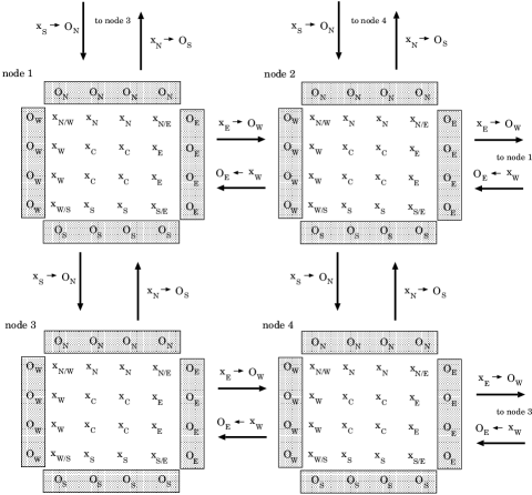
Figure 3: Internal parallelization of a $8\times 8$ lattice with periodic boundary conditions lattice on 4 node system.

for an $8\times 8$ lattice. Each node administers the data points of a $4\times 4$ sub-lattice (denoted by crosses) as well as the current values of the surface points of the neighboring sub-lattices (denoted by O). After each iteration step of the solver, e.g. MR, the updated values of each sub-lattice ($X_{N},X_{S},X_{W},X_{E}$) are passed to the “O-buffers” of the neighboring sub-lattices, i.e. $X_{S}\rightarrow O_{N},X_{N}\rightarrow O_{S}$ etc. . This procedure is repeated until some stopping criterion, set by e.g. an upper bound of the norm of the rest vector, is fulfilled.

The “internal parallelization” requires of course a communication network of much higher quality than the “external parallelization”. Although the amount of data which has to be exchanged between the nodes after each iteration step can be adjusted by a suitable choice of the sub-lattice size, the number of communications necessary to complete one full estimate can not: It is determined by the number of iterations needed by the solver to converge. Typically, this number is in the range of a few hundred for $\kappa$ values in a physically interesting region. Thus, the startup time for the communication has to be taken seriously into account.

We mention that the memory overhead introduced by the “O-buffers” can be avoided on shared memory machines. On such a machine each processor reads the required data directly from the memory of the neighboring nodes.

Finally, we emphasize that “external” and “internal” parallelization can be mixed. In this case one would divide the total of nodes into subgroups, on which one would implement “internal” parallelization. These subgroups could then run essentially independent of each other, in the “external” mode, to work at different estimates. An advantage of such a mixed solution is that one needs fast communication only within the subgroups. Furthermore, one would achieve more flexibility in optimizing the ratio of communication to CPU time on a given set of nodes.

6 What has been achieved so far

The evaluation of disconnected contributions with stochastic estimator methods is still at its beginning. Clearly, this is due to the requirement of a very high computer speed needed to tackle such a problem.

Pioneering studies of disconnected contributions have been performed some time ago on conventional (vector) computers in the quenched approximation of QCD, where one neglects the fermionic quantum fields in the Monte Carlo update, by the authors of refs. japan_nsigma ; japan_ga and liu_nsigma ; liu_ga . Due to the lack of computer speed, the authors had to make concessions to the statistical reliability of their results. Thus, although the data look promising, a systematic bias of their findings cannot be excluded.

With the advent of powerful parallel computers it became possible to treat disconnected contributions more reliably sesam_nsigma ; sesam_disc ; sesam_ga ; kilcup , although one is still limited to medium size lattices.

So far, the most intense study of such contributions has been performed by the SESAM collaboration sesam_nsigma ; sesam_ga on a QH2 APE-100 computer rapuano_here which runs the stochastic estimator code with a sustained speed of $\simeq 6$ Gflops. SESAM has analyzed 200 full QCD quantum field configurations of a $16^{3}\times 32$ lattice, at several values of the mass parameter $\kappa$. On each configuration, and for each $\kappa$, the values of $D_{1}$ and $D_{\gamma_{3}\gamma_{5}}$ have been estimated 400 times.

The statistical analysis of the SESAM data revealed that the related physical quantities, i.e. the correlation $C_{\Gamma}$ of $D_{\Gamma}$ and the proton propagator with respect to the quantum field configurations, can be determined within an uncertainty of $30\%$ for $C_{1}$ and $50\%$ for $C_{\gamma_{3}\gamma_{5}}$ within this setup.

Clearly, this is not satisfactory. But, as we pointed out above, the use of stochastic estimator techniques is still in its infancy. The SESAM result sets the stage of what has to be invested to achieve the goal of calculating disconnected contributions within a few percent uncertainty.

Besides the expected increase of computational power over the next years, improvements of the stochastic estimator technique will help to increase the statistical significance in the calculation of disconnected amplitudes. Promising suggestions along this line can be found in philippe and viehoff_dolby .

7 Summary

We have illustrated that the calculation of disconnected contributions with stochastic estimator methods represents a computationally very hard problem in lattice QCD.

Fortunately, there are several straightforward ways to implement the code on a parallel computer. Thus, almost every powerful parallel machine can be used.

In view of the intrinsic parallelism of the problem with respect to the number of estimates, the ideal computer to run the code for medium size lattices is a large cluster of workstations.

References

- (1) N. Metroprolis, A.W. Rosenbluth, M.N. Rosenbluth, A.H. Teller, and E. Teller: Equation of State Calculations by Fast Computing Machines, J. Chem. Phys.21 (1953)1087; N. Cabibbo and E. Marinari: A New Method for Upadating Matrices in Computer Simulations of Gauge Theories, Phys. Lett. 119B (1982)387; K. Fabricius and O. Haan: Heat Bath Method for the Twisted Eguchi-Kawai Model, Phys. Lett. B143 (1984)459; A. Kennedy and B. Pendleton: Improved Heat Bath Method for Monte Carlo Calculations in Lattice Gauge Theories, Phys. Lett. B156 (1985)393; M. Creutz: Overrelaxation and Monte Carlo Simulation, Phys. Rev. D36 (1987)515.
- (2) S. Duane, A.D. Kennedy, B.J. Pendleton, and D.Roweth: Hybrid Monte Carlo, Phys. Lett. B 195 (1987)216; M. Lüscher: A New Approach to the Problem of Dynamical Quarks in Numerical Simulations of Lattice QCD, Nucl. Phys. B418 (1994) 637.
- (3) A.D. Kennedy: The Hybrid Monte Carlo Algorithm on Parallel Computers, this volume.
-
(4)
For recent reviews see:
G.M. Shore: The ’Proton Spin’ Effect: Theoretical Status ’97, Nucl. Phys. Proc. Suppl. 64 (1998)167;
H.-J. Cheng: Status of the Proton Spin Problem, Int. J. Mod. Phys. A11 (1996)5109;
M. Anselmino, A. Efremov, and E. Leader: The Theory and Phenomenology of Polarized Deep Inelastic Scattering, Phys. Rep. 261 (1995)1, erratum ibid. 281 399 (1997). - (5) G. t’Hooft: Computation of the Quantum Effects due to a Four-Dimensional Pseudoparticle, Phys. Rev. D14 (1976)3432, erratum ibid. D18 2199 (1978); E. Witten: Current Algebra Theorems for the ’Goldstone Boson’, Nucl. Phys. B156 (1979)269; G. Veneziano: U(1) without Instantons, Nucl. Phys. B159 (1979)213.
- (6) R. Burkhalter: Recent Results from the CP-PACS Collaboration, hep-lat/9810043, Nucl. Phys. B (Proc. Suppl.) 1999, in print.
- (7) R. Gupta: General Physics Motivations for Numerical Simulations of Quantum Field Theory, this volume.
- (8) J. Gasser, H. Leutwyler, and M.E. Sainio: Sigma Term Update, Phys. Lett. B253(1991)252; J. Gasser, H. Leutwyler, and M.E. Sainio: Form-Factor of the Sigma Term, Phys. Lett. B253 (1991)260.
- (9) T. Lippert: Parallel SSOR Preconditioning for Lattice QCD, this volume.
- (10) K. Bitar, A.D. Kennedy, R. Horsley, S. Meyer, and P. Rossi: Hybrid Monte Carlo and Quantum Chromodynamics, Nucl. Phys. B313 (1989)348.
- (11) S.J. Dong and K.F. Liu: Quark Loop Calculations, Nucl. Phys. B(Proc. Suppl.)26 (1992)353.
- (12) S.J. Dong and K.F. Liu: Stochastic Estimation with Noise, Phys. Lett. B328 (1994)130.
- (13) SESAM Collaboration, S. Güsken, P. Ueberholz, J. Viehoff, N. Eicker, P. Lacock, T. Lippert, K. Schilling, A. Spitz, and T. Struckmann: The Pion Nucleon Sigma Term with Dynamical Wilson Fermions, Phys. Rev. D59, 054504 (1999).
- (14) SESAM Collaboration, N. Eicker, U. Glässner, S. Güsken, H. Hoeber, T. Lippert, G. Ritzenhöfer, K. Schilling, G. Siegert, A. Spitz, P. Ueberholz, and J. Viehoff: Evaluating Sea Quark Contributions to Flavour-Singlet Operators in Lattice QCD, Phys. Lett. B389 (1996)720.
- (15) For an overview see Web-page http://www.ncsa.uiuc.edu/Apps/CMP/RNG/
- (16) M. Fukugita, Y. Kuramashi, M. Okawa, and A. Ukawa: Pion - Nucleon Sigma Term in Lattice QCD, Phys. Rev. D51 (1995)5319.
- (17) M. Fukugita, Y. Kuramashi, M. Okawa, and A. Ukawa: Proton Spin Structure from Lattice QCD, Phys. Rev. Lett. 75 (1995)2092.
- (18) S.J. Dong, J.F. Lagaë, and K.F. Liu: Pi N Sigma Term, Anti-S S in Nucleon, and Scalar Form-Factor: A Lattice Study, Phys. Rev. D54 (1996)5496; S.J. Dong and K.F. Liu, Nucl. Phys. B (Proc. Suppl.)42 (1995)322.
- (19) S.J. Dong, J.F. Lagaë, and K.F. Liu: Flavor Singlet g(A) from Lattice QCD, Phys. Rev. Lett. 75 (1995)2096.
- (20) SESAM Collab., S. Güsken, P. Ueberholz, J. Viehoff, N. Eicker, T. Lippert, K. Schilling, A. Spitz, and T. Struckmann: The Flavor Singlet Axial Coupling of the Proton with Dynamical Wilson Fermions, preprint WUB98-44, HLRZ 1998-85, hep-lat/9901009, Phys. Rev. D. in print.
- (21) L. Venkataraman and G. Kilcup: The Meson with Staggered Fermions, hep-lat/9711006.
- (22) F. Rapuano: Physics on APE Computers, this volume.
- (23) Ph. de Forcrand: Monte Carlo Quasi-Heatbath by Approximate Inversion, Phys. Rev. E 59 (1999)3698.
- (24) SESAM Collaboration, J. Viehoff et al.: News on Disconnected Diagrams, hep-lat/9809130, to be published in Nucl. Phys. (Proc. Suppl.) 1999.