The Conformal Mode in 2D Simplicial Gravity

Abstract

We verify that summing 2D DT geometries correctly reproduces the Polyakov action for the conformal mode, including all ghost contributions, at large volumes. The Gaussian action is reproduced even for $c_{m}=10$, well into the branched polymer phase, which confirms the expectation that the DT measure is indeed correct in this regime as well

Introduction. In the last decade there has been considerable progress in our understanding of two dimensional quantum gravity (2DQG). The key element that has made this progress possible is the recognition that the trace anomaly requires the effective action of 2DQG to be augmented by a well-defined nonlocal term [1],

$$S_{anom}={Q^{2}\over 16\pi}\int d^{2}x\sqrt{-g}\int d^{2}x^{\prime}\sqrt{-g^{\prime}}\ R(x)\ \lower 0.6458pt\hbox{$\Box$}^{-1}(x,x^{\prime})\ R(x^{\prime})\ .$$ (1)

Because this action is conformally invariant, and the massless scalar propagator $\lower 0.6458pt\hbox{$\Box$}^{-1}(x,x^{\prime})\sim\log(x-x^{\prime})^{2}$ in two dimensions, $S_{anom}$ is relevant (strictly, marginal) in both the infrared and ultraviolet, and leads to nontrivial scaling of the distribution of random geometries in the path integral for 2DQG.

This scaling behavior has been found analytically in the continuum, both by canonical operator methods for the current algebra of the energy-momentum tensor [2], and by covariant conformal field theory methods for the Euclidean correlation functions [3]. The former KPZ approach exposes the relation of the parameter $Q^{2}$ to the unique central extension of the current algebra of diffeomorphisms on the 2D world sheet,

$$Q^{2}={25-c_{m}\over 6}\ ,$$ (2)

where $c_{m}$ is the central charge of the matter representation. For free matter $c_{m}$ is the integer number of free boson or fermion fields: $c_{m}=N_{s}+N_{f}$. The value of $Q^{2}={25\over 6}$ for $c_{m}=0$ is the value for pure 2DQG.

The second covariant approach to 2DQG is more closely related to the statistical properties of the ensemble of 2D geometries, and may be checked by a numerical Monte Carlo method applied to a discretized Euclidean worldsheet [4]. In this approach fluctuations of the worldsheet are modelled by performing a sum over a set of dynamical triangulations (DTs). The DT numerical simulations agree with the continuum scaling predictions in all important respects [5]. In particular, correlation functions of conformal operators acquire well-defined anomalous scaling dimensions, which can be computed in terms of $Q^{2}$ and agree with (2), including the miminal models for which $c_{m}=1-6/n(n+1)<1$, where $n$ is an integer $n\geq 2$. What is remarkable about this agreement is that the anomalous action (1) which gives rise to the ‘gravitational dressing’ of conformal operators in the continuum is not inserted into the discretized action of the DT simulation by hand, but instead must be generated automatically with the correct coefficient by the integration measure on the space of geometries in the DT approach.

Despite the satisfactory agreement between theory and the DT approach for correlation functions in 2DQG, one would like to demonstrate explicitly the appearance of $e^{S_{anom}}$ in the measure of 2DQG, particularly for $c_{m}>1$, where the continuum scaling relations become complex and the interpretation of the theory becomes much less clear. This is our main purpose in this Letter.

For studying this question in more detail it is useful to introduce the conformal parameterization of the metric,

$$g_{ab}=e^{2\sigma}\bar{g}_{ab}\ ,$$ (3)

where $\bar{g}_{ab}$ is a fixed fiducial metric which depends only on the global topology of the two dimensional Euclidean manifold. Since all two-manifolds are locally conformally flat, there is a local coordinate patch around every point where the fiducial metric has the form $\delta_{ab}$. A finite number of such coordinate patches and global (Teichmuller) moduli parameters are required to describe the fiducial metric in any given topology, but all local deformations of $g_{ab}$ are contained in the conformal factor $e^{2\sigma(x)}$. The Ricci scalar is given by

$$R=e^{-2\sigma}(\overline{R}-2\lower 1.07639pt\hbox{$\stackrel{{\scriptstyle\mbox{\rule[1.70717pt]{6.82864pt}{0.36989pt}}}}{{\Box}}$}\sigma)=e^{-2\sigma}\overline{R}-2\lower 0.6458pt\hbox{$\Box$}\sigma$$ (4)

in the parameterization (3), where the overbars refer to the fiducial metric $\bar{g}_{ab}$ and the absence of an overbar refers to the full metric $g_{ab}$. It is a theorem in 2D Riemannian geometry that for any smooth manifold with given continuous $R(x)$, a unique solution to the nonlinear equation for $\sigma$ (4) exists such that $\overline{R}$ is everywhere a specified constant [6]. This constant is necessarily positive for closed manifolds with no handles, i.e. with the topology of the sphere $S^{2}$, zero for closed manifolds with one handle, i.e. with the topology of the torus $T^{2}$ and negative for closed manifolds with more than one handle. The uniformization (Yamabe) theorem assures us that we can construct the conformal factor $e^{\sigma(x)}$ uniquely for every 2D closed manifold of fixed topology.

In the conformal parameterization and Euclidean signature the action $S_{anom}$ becomes

$$S_{E}[\sigma]=-S_{anom}={Q^{2}\over 4\pi}\int d^{2}x\ \sqrt{{\bar{g}}}\ \bigl{[}\sigma(-\,\lower 1.07639pt\hbox{$\stackrel{{\scriptstyle\mbox{\rule[1.70717pt]{6.82864pt}{0.36989pt}}}}{{\Box}}$})\,\sigma+\overline{R}\sigma\bigr{]}+const.$$ (5)

which is local and quadratic in $\sigma$. Hence in this variable the distribution of geometries in the path integral for 2DQG is the same as that of a free scalar field with a well-defined normalization. As long as $Q^{2}$ is positive this Gaussian distribution is bounded on closed Riemannian manifolds, as is clear upon integration of the quadratic term in (5) by parts.

Smooth geometries and the classical limit to 2DQG are recovered only in the large $Q^{2}$ limit, $Q^{2}\to\infty$ ($c_{m}\to-\infty$), where the fluctuations in the conformal factor become suppressed. The $25$ in (2) for pure 2DQG can be understood in the conformal gauge as arising from $26$ from the ghosts of Faddeev-Popov gauge fixing and $-1$ for $\sigma$ field itself, which contributes to the anomalous action as would one additional matter scalar degree of freedom, lowering the effective value of $Q^{2}$. Although the KPZ scaling relations become complex for $c_{m}>1$, nothing singular occurs in the action $S_{E}$ as $c_{m}$ is raised above $1$ and $Q^{2}$ is lowered below $4$, However, a heuristic argument based on the competition of action and entropy of singular ‘spike’ solutions to the classical equations following from $S_{E}$ suggests that at the critical value $Q_{cr}^{2}=4$ the theory undergoes a BKT-like phase transition [7] to a phase dominated by elongated extrusions of the 2D world sheet, since the entropy of these configurations first exceeds their action at this value of $Q^{2}$ [8]. Hence for $Q^{2}\leq Q_{cr}^{2}$, the typical 2D geometry would be expected to be very far from smooth, resembling instead a multiply branched polymer. This branched polymer phase is seen also in the DT simulations for $c_{m}>1$ [9].

The significance of the critical value, $c_{m}=1$ may also be understood from a canonical perspective on Lorentzian signature 2D manifolds. In the absence of matter the quadratic theory specified by the anomalous action $S_{anom}$ is overconstrained. This is clear from the fact that the metric is a $2\times 2$ symmetric matrix which has three independent components, $g_{00},g_{11}$ and $g_{01}=g_{10}$. Two of these are isomorphic to pure gauge diffeomorphisms of the 2D worldsheet and can be removed. This leaves one independent componen which can be taken to be the conformal mode $\sigma$, but its dynamics is constrained by the two first class constraints in the $(00)$ and $(01)$ components of the Euler-Lagrange equations following from $S_{anom}$. These are the 2D lapse and shift constraints to be imposed on the phase space in the canonical treatment of a theory with diffeomorphism invariance. Hence there are finally $3-2-2=-1$ local degrees of freedom in pure 2DQG described by the Polyakov action (1), or in other words the theory is overconstrained and possesses no local degrees of freedom. When free matter fields are added the theory has $c_{m}-1$ local degrees of freedom and the conformal mode first can fluctuate locally when $c_{m}\geq 1$, which coincides with the BKT phase transition critical value, $Q^{2}\leq Q^{2}_{cr}=4$ In this branched polymer phase where the conformal spike configurations become ‘liberated,’ 2DQG becomes sensitive to its UV cutoff and a smooth continuum limit at large distance scales presumably does not exist, unless higher derivative UV relevant operators or an explicit UV cutoff are introduced.

In the DT discretized approach to 2DQG the UV cutoff is supplied by the lattice scale $a$, while the IR behavior is controlled by the total 2D volume, i.e. the sum of areas of all the triangles in the ensemble. If the interpretation of the $c_{m}=1$ ‘barrier’ given above is correct we would expect the distribution of $\sigma$ fields on the lattice to remain Gaussian with a well-defined width determined by $S_{E}$ in the large volume limit, even in the branched polymer phase where the typical geometries are irregular on the lattice scale. To check this hypothesis requires finding the conformal factor by solving the Yamabe equation (4) on each geometry in the DT ensemble and reconstructing the distribution of $\sigma$ in the ensemble. Besides casting some light on the case $c_{m}\geq 1$ the construction of this Gaussian distribution in $\sigma$ would provide explicit confirmation of the identity of the continuum and lattice approaches, independently of any correlation functions or expectation values of observables. Preliminary studies of this distribution were reported in Refs. [10, 11].

We have an additional motivation for the construction of this distribution in $\sigma$ from the analysis of the conformal anomaly generated action in 4D. At the infrared fixed point of this 4D action the conformal factor distribution is again predicted to be Gaussian with a width determined by the analogous anomaly coefficient in 4D [12]. In the conformal parameterization (3) the 4D action analogous to (5) is

$$S_{E}[\sigma]_{D=4}={Q^{2}\over(4\pi)^{2}}\int d^{4}x\sqrt{g}\,\bigl{[}\sigma{\Delta}_{4}\sigma+\hbox{$1\over 2$}\bigl{(}G-\hbox{$2\over 3$}\lower 0.6458pt\hbox{$\Box$}R\bigr{)}\sigma\bigr{]}\ ,$$ (6)

with the contribution to the coefficient from the number of massless conformal scalar ($N_{S}$), Weyl fermion ($N_{WF}$) and vector ($N_{V}$) fields given by

$$Q^{2}_{D=4}={1\over 180}(N_{S}+\hbox{$11\over 2$}N_{WF}+62N_{V}-28)+Q^{2}_{grav}\ ,$$ (7)

and $Q^{2}_{grav}$ the contribution of gravitons. In (6) $G$ is the Gauss-Bonnet invariant and $\Delta_{4}=\lower 0.6458pt\hbox{$\Box$}^{2}+2R^{ab}\nabla_{a}\nabla_{b}-{\textstyle\frac{2}{3}}R{\lower 0.6458pt\hbox{$\Box$}}^{2}+{\textstyle\frac{1}{3}}(\nabla^{a}R)\nabla_{a}$ is the unique fourth order conformally covariant operator in 4D which has a logarithmic propagator, analogous to $\Box$ in 2D. The action (6) is therefore relevant (strictly, marginal) in the IR and leads to nontrivial scaling of the cosmological and Newtonian ‘constants’ at large distance scales [13]. These scaling relations become complex for $Q^{2}_{D=4}<8$, analogous to $Q^{2}<4$ in 2D, with the important difference that additional matter fields take us into the smooth phase in 4D but the irregular branched polymer phase in 2D, since matter contributes positively in (7) but negatively in (2). Moreover, singular ‘spike’ solutions also exist in this 4D conformal theory and their entropy exceeds their action at precisely the same critical value at which the scaling relations become complex [14].

Since the DT program in 4D has not met with the same level of success as in 2D, it would be an important check on the model to construct the distribution of the conformal factors generated by the DT algorithm to determine if it is consistent with the continuum trace anomaly and action (6) in 4D. A positive result would provide a method of determining the contribution of the gravitons $Q^{2}_{grav}$ to the Gaussian width as well. Clearly the situation is quite a bit more complicated in 4D and will require a careful disentangling of the graviton degrees of freedom in addition to $\sigma$, but the basic idea of the reconstruction of the metric of each member of the DT ensemble is similar in higher dimensions, and the method should be tested first in the 2D case which is the most complete and best understood model of QG which we have at the present time.

Dynamical Triangulations. In the dynamical triangulation approach to 2DQG one constructs an ensemble of discretized geometries, each one of which consists of regular two-simplices, i.e. equilateral triangles, glued together at their edges. If the length of any side of one of the triangles is $a$ then its area is $A_{\Delta}=\sqrt{3}a^{2}/4$. If $N_{0}=N$ is the total number of vertices in the lattice then the total number of links is $N_{1}=3(N-\chi_{{}_{E}})$ and the total number of triangles is $N_{2}=2(N-\chi_{{}_{E}})$, where

$$\chi_{{}_{E}}={1\over 4\pi}\int\ d^{2}x\sqrt{g}\ R\to\sum_{i}\left(1-{q_{i}\over 6}\right)=N_{0}-{N_{1}\over 3}$$ (8)

is the Euler character of the triangulation and $q_{i}$ is the coordination number of the vertex $i$, i.e. the number of neigboring vertices to which it is connected by a single link. Hence $\sum_{i}q_{i}=2N_{1}$ since each link is counted twice in this sum. In the following we restrict ourselves to spherical topology $S^{2}$ for which $\chi_{{}_{E}}=2$.

In the dual lattice the area of the cell associated with the vertex $i$ is

$$(d^{2}x\sqrt{g})_{i}\to\tilde{A}_{i}={q_{i}\over 3}A_{\Delta}\ ,$$ (9)

and the scalar curvature concentrated at the vertex $i$ is

$$R_{i}\to{2\pi\over q_{i}A_{\Delta}}(6-q_{i})\ ,$$ (10)

which together are consistent with (8). When $q_{i}=6$ the vertex has no curvature associated with it, since $6$ equilateral triangles joined at the vertex tile a local region of flat space.

The scalar Laplacian on the lattice site $i$ can be represented as a sum over its $q_{i}$ nearest neighbors $j(i)$ as [15]

$$(-\lower 0.6458pt\hbox{$\Box$}\sigma)_{i}\to{2\sqrt{3}\over q_{i}A_{\Delta}}\sum_{j(i)}(\sigma_{i}-\sigma_{j})={2\sqrt{3}\over q_{i}A_{\Delta}}\sum_{j}(q_{i}\delta_{ij}-C_{ij})\sigma_{j}\ ,$$ (11)

where $C_{ij}$ is the coordination or adjacency matrix, equal to one if $i$ and $j$ are connected by a single link and zero otherwise. Hence the Yamabe equation (4) on the lattice becomes

$$2M_{ij}\sigma_{j}=\frac{2\pi}{3}\left(6-q_{i}\right)-\frac{\overline{R}q_{i}}{3}\,A_{\Delta}\,e^{-2\sigma_{i}}$$ (12)

after multiplication through by $\tilde{A}_{i}$. Here, we have defined the matrix,

$$M_{ij}=\frac{2}{\sqrt{3}}\left(q_{i}\delta_{ij}-C_{ij}\right)\$$ (13)

The left side of Eq. (12) vanishes when summed over $i$. Hence we obtain the constraint,

$$8\pi=\frac{\overline{R}\,A_{\Delta}}{3}\sum_{i}q_{i}e^{-2\sigma_{i}}=\overline{R}\,A_{\Delta}\,N_{2}\ ,$$ (14)

where the last relation follows from the lattice version of $\int\sqrt{g}e^{-2\sigma}=\int\sqrt{\bar{g}}\to A_{\Delta}N_{2}$. Thus if $\overline{R}$ is held constant in the continuum limit, $N_{2}\to\infty$ and $A_{\Delta}\sim 1/N_{2}\to 0$. This implies that we scale the lattice spacing to zero like the inverse square root of the number of triangles.

The ensemble of configurations for the fixed area partition function is generated by a Monte Carlo simulation which updates the geometry at fixed large $N_{2}$ using link flips with unit probability, i.e. no gravitational action is used to weight the configurations. To couple matter we just dress the vertices with $c_{m}$ free scalar fields coupled by the usual Gaussian action using the scalar Laplacian (11). A combined heat bath and overrelaxation algorithm was used to simulate the scalars. For each of the runs we generated $10,000$ configurations separated by 100 Monte Carlo sweeps. Lattices of size with $N_{2}=100,\,200,\,400,\,800,\,$ and $1600$ triangles were used.

For each configuration in the ensemble the conformal mode was constructed by solving (13) by a modified Newton-Raphson iteration scheme. In order to compare the results with the anomalous action $S_{anom}$ the conformal mode is decomposed into eigenmodes of the round sphere Laplacian, $-\lower 1.07639pt\hbox{$\stackrel{{\scriptstyle\mbox{\rule[1.70717pt]{6.82864pt}{0.36989pt}}}}{{\Box}}$}=-\frac{\sqrt{g}}{\sqrt{\overline{g}}}\lower 0.6458pt\hbox{$\Box$}=-e^{2\sigma}\lower 0.6458pt\hbox{$\Box$}$. A symmetrized version of this operator on the lattice can be defined by

$$L_{ij}={3\over A_{\Delta}}{e^{\sigma_{i}+\sigma_{j}}\over\sqrt{q_{i}q_{j}}}M_{ij}$$ (15)

The spectrum $\{\lambda^{\ell}\}$ and eigenmodes $\{u^{\ell}_{i}\}$ of this operator were computed,

$$L_{ij}u^{\ell}_{j}=\lambda_{\ell}\,u^{\ell}_{i}\ ,$$ (16)

with the modes taken to be orthonormal with respect to a measure which is just the lattice version of $\sqrt{\overline{g}}=\frac{q_{i}}{3}e^{-2\sigma_{i}}A_{\Delta}$. Finally the overlap of $\sigma_{i}$ on this set of modes $u_{i}^{\ell}$ was computed, using the expression,

$$\sigma^{\ell}=\int\,d^{2}x\,\sqrt{\overline{g}}\,u^{\ell}\,\sigma\to\sum_{i}\tilde{A}_{i}\,e^{-2\sigma_{i}}\,u^{\ell}_{i}\,\sigma_{i}\,\ .$$ (17)

It is often convenient in numerical calculations to work with dimensionless quantities $\sigma^{\ell}_{\rm latt}={A_{\Delta}}^{-\frac{1}{2}}\sigma^{\ell}$ and $\lambda_{\ell\,\rm latt}=A_{\Delta}\lambda_{\ell}$ corresponding to the operator $A_{\Delta}L_{ij}$ and lattice measure $\frac{q_{i}}{3}e^{-2\sigma_{i}}$.

According to the Polyakov-Liouville action $S_{anom}$, the amplitude of each mode should be distributed as

$$\exp\left\{-{Q^{2}\over 4\pi}\sum_{\ell}\lambda_{\ell}\left(\sigma^{\ell}\right)^{2}\right\}$$ (18)

To check this we rescaled each amplitude $\sigma^{\ell}$ by multiplying by $(\lambda_{\ell})^{{1\over 2}}$ and calculated the frequency distribution for this rescaled (dimensionless) amplitude. All rescaled mode distributions should fit to a Gaussian with constant width determined only by $Q^{2}$

In addition one can examine the zero mode amplitude $\sigma^{0}$. This should be governed by just the linear term in the action $S_{anom}$ (eqn. 5). This distribution is predicted to be (ignoring the fixed area constraint)

$$P\left(\sigma^{0}_{\rm latt}\right)\sim\exp\left\{-\frac{2Q^{2}}{\sqrt{N_{2}}}\sigma^{0}_{\rm latt}\right\}$$ (19)

The inclusion of the fixed area constraint (eqn. 14) leads to a more complicated distribution for the zero mode. However this constraint has little effect for large amplitudes where we expect a simple exponential behavior.

Numerical Results. We show data for both pure 2DQG ($c_{m}=0$) below the critical value of $c_{m}=1$ and for 2DQG coupled to ten free massless scalar fields ($c_{m}=10$) - well above the critical value. The fits to a Gaussian distribution in $\sigma$ are shown in Fig. 1 and Fig. 2 respectively. For $c_{m}=0$ the fitted width using (rescaled) mode $\ell=10$ is $w=1.735(10)$ and corresponds very closely to the value expected from the Liouville action $w^{L}(c_{m}=0)=\sqrt{\frac{24\pi}{25-c_{m}}}\simeq 1.7368$. Similarly the fitted width for (rescaled) mode $\ell=8$ at $c_{m}=10$ is $w=2.195(15)$ which lies just 3 standard deviations away from its predicted value $w^{L}(c_{m}=10)=2.2420$. We attribute the small discrepancy in the latter to the presence of finite size effects which appear somewhat larger for more scalar degrees of freedom.

To examine both the finite size and mode dependence effects more closely we have plotted in Figs. 3 and 4 the dependence of the rescaled width on lattice eigenvalue $\lambda_{\rm latt}$, for volumes $N_{2}=500$ through $N_{2}=1600$. All points correspond to $\chi^{2}$ per d.o.f. of unity or less. Errors on histograms were obtained using a bootstrap technique. Notice first that the (rescaled) widths are relatively insensitive to the eigenvalue of the lattice Laplacian and within 10 per cent of so of the Liouville prediction, which is indicated by the solid horizontal extending away from the y-axis. If we focus attention on any curve corresponding to a single volume, we notice that for small eigenvalue it climbs steeply to reach a broad peak (close to the continuum prediction as indicated by the solid line). Thereafter it falls very slowly with increasing eigenvalue. Clearly both lattice cut-off effects and finite size effects play a role in determining the precise shape of the curve. This is especially true deep into the branched polymer phase with $c_{m}=10$ in Fig. 4, where the typical geometries are very irregular on the lattice scale $a$. We should expect the lattice Laplacian to depart significantly from the continuum there, with the higher modes suffering systematic deviations.

For the lower eigenvalues the fixed volume constraint which we have neglected to this point must also be taken into account. In the continuum partition function this amounts to the insertion of the delta function constraint, $\delta\left(A-\int\sqrt{\overline{g}}e^{\alpha\sigma}\right)$ into the functional integral governed by the action (6). In the DT simulation this constraint enters through (14) for the background area. Clearly this constraint couples all the modes nonlinearly and causes their distribution to depart from a Gaussian, although it is natural to expect its effects will be larger on modes with the longest wavelengths. In the continuum limit, defined by the process of taking the average triangle size $A_{\Delta}\to 0$ while holding $\bar{R}$ and the continuum eigenvalue fixed, the effect of the constraint becomes unimportant. In this limit we should examine the behavior of the eigenvalue curves for small lattice eigenvalue. The finite size effects enforced by the constraint (14) prevent us from going literally to zero lattice eigenvalue, and are responsible for the rapid turn over of the curves at the smallest eigenvalues in Figs. 3 and 4. It is clear that for small enough (lattice) eigenvalue the wavelength of a mode saturates at the typical linear size and hence the rescaled width goes to zero like the square root of the lattice eigenvalue. Thus any extrapolation procedure should utilize the smallest eigenmodes with long wavelengths that are still significantly smaller than the lattice size. The trend of the curves in Figs. 3 and 4 with increasing volume indicates that the modes whose widths lie close to the peak are candidates for such ‘continuum-like’ eigenmodes. Indeed the heights of these peaks show a convergence to the value expected from the continuum Gaussian theory.

One way to check this conclusion (and the self-consistency of the numerical calculations) is to consider the effect of using massive rather than massless scalar fields. Fig. 5 shows a plot of the width versus eigenvalue for a lattice with volume $N_{2}=1600$ as a function of scalar field mass $M$. The (lattice) mass parameter was set at $1.0$, $0.1$ and finally $0.01$. We see that for lattice eigenvalues $a_{\Delta}\lambda>1$ all the curves are statistically similar and compatible with the data for $M=0.0$ (Fig. 4). In this region of the spectrum the lattice cannot distinguish massless from massive, and the lattice cut-off effects dominate. However, at smaller eigenvalues $a_{\Delta}\lambda<1$ we see very different behavior for different masses. The widths for $M=1.0$ start to differ markedly from $M=0.1$ and $M=0.01$, the latter two curves themselves splitting apart for small enough eigenvalue $a_{\Delta}\lambda<0.25$. We can understand this behavior by realizing that the scalar fields will look effectively massless when their correlation length $1/M$ is larger than the typical linear extent of the geometries (determined by the fixed volume). Hence the $M=0.01$ curve is statistically consistent with the exactly massless data (Fig. 4) over the entire spectrum. Its peak sits close to the value expected for ten massless scalars $c_{m}=10$. In contrast the data for $M=0.1$ shows a small but significant deviation from the massless case at the smaller eigenvalues near the peak, which is consistent with the continuum correlation length $1/M$ being slightly smaller than the typical linear extent of the geometries. In this region of the spectrum the modes have a wavelength greater than $M^{-1}$ but less than the linear extent of a typical geometry in the DT ensemble. The smaller width of the Gaussian fit for these modes is consistent with the expectation that the massive modes should begin to decouple from the trace anomaly in the infrared large volume limit, yielding an effective value of $c_{m}$ smaller than that for $10$ massless scalars. For $M=1.0$ the continuum peak is not observed at all for small eigenvalues, the effects of lattice cut-off and finite volume apparently contaminating the signal even at intermediate wavelengths. Although at this mass the lattice is a bit too crude to be completely convincing, the data for $M=1.0$ is more consistent with the width expected for pure gravity rather than for gravity coupled to ten massless scalars, suggesting the complete decoupling of these very massive fields from the continuum anomalous effective action (1) at this volume. For all masses at the largest wavelengths (smallest eigenvalues) where finite size effects should dominate, the curves eventually turn over and head towards zero.

Thus the massive simulations support our preliminary conclusion that continuum physics is obtained at small eigenvalue close to the peak in the width vs. eigenvalue plots, where both lattice and finite volume effects are minimized. However it would be fair to say that we do not have a completely satisfactory quantitative understanding of these lattice and finite size effects, in the absence of which one may question the complete exclusion of the larger eigenvalue region of the plots. If the shape of curve is dominated by lattice effects at all but the longest wavelengths it is reasonable to consider the ratio of widths between $c_{m}=0$ and $c_{m}=10$ theories over the entire eigenvalue range, expecting the leading systematic lattice effects to drop out of this ratio. A plot of this ratio is shown in Fig. 6 which supports this idea. The fluctuations in the measured ratio vary by only a few percent over all eigenvalues excluding the very lowest. Moreover, the ratio of Gaussian widths is consistent with that expected from the continuum action, $\sqrt{25-10\over 25}\simeq 0.7746$.

Finally the action (1) also predicts the asymptotic form of the zero mode distribution to be a simple exponential, controlled by the linear term in (6), again if the effects of the finite volume constraint (14) is ignored. From (14) we expect that the distribution of $\sigma_{0}$ should become exponentially insensitive to the constraint for large $\sigma_{0}$. A fit for large values of the zero mode amplitude $\sigma_{0}$ of the logarithm of its distribution for $c_{m}=0$ is shown in Fig. 7. The data corresponds to a simulation with $N_{2}=800$ simplices. The slope of $0.304(10)$ compares well with the expected value from the continuum, $0.295$. The same mode for $c_{m}=10$ is also shown in Fig. 8. Here there are fewer points and their errors are substantially larger, consistent with larger finite size effects, but again the slope of $0.24(2)$ does not differ too badly from the continuum prediction of $0.177$, lying approximately three standard deviations away from it.

In conclusion, we have shown that is is possible to reconstruct a lattice conformal mode from the ensemble of DT geometries, even for $c_{m}>1$. We have shown that the distribution of this conformal mode is bounded and Gaussian with a width corresponding to that expected from the anomalous action (1), even well into the branched polymer phase. This provides an explicit connection between the ensemble of geometries generated by the DT method and the continuum quantization of 2D gravity. The correspondence between the DT lattice and continuum approaches demonstrates that the DT measure generates automatically the correct anomaly coefficient $Q^{2}$ including the Faddeev-Popov ghost contributions in the continuum. This is a non-trivial result since it implies DTs can be used to study 2D gravity even in the regime where the KPZ exponents become complex, and the theory becomes sensitive to its UV cut-off. Finally, the massive scalar simulations support the proposition that the anomaly generated action (1) is indeed the correct effective Wilsonian action in the continuum large volume (infrared) limit, where massive states should decouple.

Acknowledgments The authors would like to thank Tanmoy Bhattacharya for useful discussion. This work was supported in part by DOE grant DE-FG02-85ER40237. Simon Catterall would like to thank the T-8 group at Los Alamos National Laboratory where much of this work was carried out.

FIG. 1.: Gaussian distribution for (rescaled) amplitude $\sigma^{\ell}$ ($\ell=10$) for pure 2DQG $c_{m}=0$ in the case of $N_{2}=1600$ simplices.

FIG. 2.: Gaussian distribution for the (rescaled) amplitude $\sigma^{\ell}$ ($\ell=8$) for 2DQG coupled to ten free scalar fields ($c_{m}=10$) in the case of $N_{2}=1600$ simplices.

FIG. 3.: The rescaled width of the Gaussian distribution in $\sigma$ vs. lattice eigenvalue $\lambda_{\rm latt}$ for pure 2DQG ($c_{m}=0$) in the case of $N_{2}=1600$.

FIG. 4.: The rescaled width of the Gaussian distribution in $\sigma$ vs. lattice eigenvalue $\lambda_{\rm latt}$ for 2DQG coupled to ten massless scalar fields ($c_{m}=10$) in the case of $N_{2}=1600$ simplices.

FIG. 5.: Width vs. eigenvalue for $N_{2}=1600$ for three different values of the lattice mass $M=0.01,0.1,1.0$.

FIG. 6.: The ratio of Gaussian widths for $c_{m}=0$ to $c_{m}=10$ vs. eigenvalue for $V=1600$. The expected continuum ratio of $\sqrt{3\over 5}$ is indicated by the solid horizontal line.

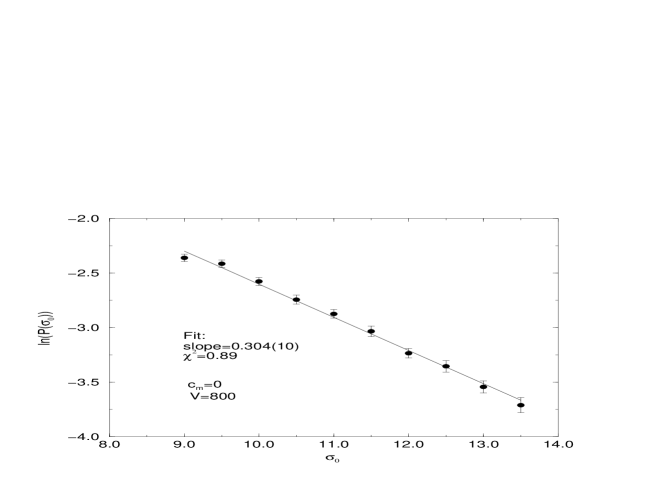
FIG. 7.: Logarithm of the zero mode distribution in $\sigma^{0}_{\rm latt}$ vs. amplitude for pure 2DQG ($c_{m}=0$).

FIG. 8.: The logarithm of the zero mode distribution in $\sigma^{0}_{\rm latt}$ vs. amplitude for gravity coupled to $c_{m}=10$ matter for $N_{2}=800$ simplices.

REFERENCES

- [1] A. M. Polyakov, Phys. Lett. B103 (1981) 207, 211; Gauge Fields and Strings (Harwood, Chur 1987).
- [2] V. G. Knizhnik, A. M. Polyakov, and A. B. Zamolodchikov, Mod. Phys. Lett. A3 (1988) 819.
- [3] F. David, Mod. Phys. Lett. A3 (1988) 1651; J. Distler and H. Kawai, Nucl. Phys. B321 (1989) 509.
- [4] J. Ambjørn, B. Durhuus, J. Frohlich and P. Orland, Nucl. Phys. B270 (1986) 457; A. Billoire and F. David, Nucl. Phys. B275 (1986) 617; D. V. Boulatov, V. A. Kazakov, I. K. Kostov and A. A. Migdal, Nucl. Phys. B275 (1986) 641.
- [5] For a review see J. Ambjørn, Nucl. Phys. Proc. Suppl. 42 (1995) 3. S. Catterall Nucl. Phys. Proc. Suppl. 47 (1996) 59.
- [6] H. Yamabe, Osaka Math. J. 12 (1960) 21; T. Aubin, Jour. Diff. Geom. 4 (1970) 383; Jour. Math. Pure & Appl. 55 (1976) 269; Nonlinear Analysis on Manifolds: Monge-Ampère Equations (Springer, New York 1982); M. S. Berger, Jour. Diff. Geom. 5 (1971) 325; R. Schoen, Jour. Diff. Geom. 20 (1984) 479.
- [7] V. I. Berezinskii, Zh. Eksp. Teor. Fiz. 59 (1970) 907 [Soviet Physics, JETP 32 (1971) 493]; M. Kosterlitz and D. Thouless, J. Phys. C6 (1973) 1181.
- [8] M.E. Cates, Europhys. Lett. 8 (1988) 719; A. Krzywicki, Phys. Rev. D41 (1990) 3086; F. David, Nucl. Phys. B368 (1992) 671;B487 (1997) 633.
- [9] J. Ambjorn, S. Jain and G. Thorleifsson Phys. Lett. B307 (1993) E. Gregory, S. Catterall and G. Thorleifsson, Nucl. Phys. 451 (1999) 285.
- [10] M. E. Agishtein and A. A. Migdal, Mod. Phys. Lett. A7 (1992) 1039; Nucl. Phys. B385 (1992) 395.
- [11] “Dynamics of the Conformal Mode and Simplicial Gravity,” S. Catterall, E. Mottola, T. Bhattacharya, hep-lat/9809114, LATTICE98 Nucl. Phys. Proc. Suppl. (1999) in press.
- [12] I. Antoniadis and E. Mottola, Phys. Rev. D45 (1992) 2013; I. Antoniadis, P. O. Mazur, and E. Mottola, Nucl. Phys. B 388 (1992) 627; S. D. Odintsov, Z. Phys. C54 (1992) 531; I. Antoniadis and S. D. Odintsov, Phys. Lett. B343 (1995) 76.
- [13] I. Antoniadis, P. O. Mazur, and E. Mottola, Phys. Lett. B444 (1998) 284.
- [14] I. Antoniadis, P. O. Mazur, and E. Mottola, Phys. Lett. B394 (1997) 49.
- [15] C. Itzykson and J.-M. Drouffe, Statistical Field Theory, Vol. 2, Cambridge Univ. Press (Cambridge, 1989).