Non-Hermitian Random Matrix Theory and Lattice QCD with Chemical Potential

Abstract

In quantum chromodynamics (QCD) at nonzero chemical potential, the eigenvalues of the Dirac operator are scattered in the complex plane. Can the fluctuation properties of the Dirac spectrum be described by universal predictions of non-Hermitian random matrix theory? We introduce an unfolding procedure for complex eigenvalues and apply it to data from lattice QCD at finite chemical potential $\mu$ to construct the nearest-neighbor spacing distribution of adjacent eigenvalues in the complex plane. For intermediate values of $\mu$, we find agreement with predictions of the Ginibre ensemble of random matrix theory, both in the confinement and in the deconfinement phase.

Physical systems which are described by non-Hermitian operators have recently attracted a lot of attention. They are of interest, e.g., in dissipative quantum chaos [1], disordered systems [2, 3], neural networks [4], and quantum chromodynamics (QCD) at finite chemical potential [5]. Often they display unusual and unexpected behavior, such as a delocalization transition in one dimension [2]. Consequently, analytical efforts have been made to develop mathematical methods to deal with non-Hermitian matrices, see, e.g., Refs. [6, 7, 8, 9, 10].

Of particular interest in the analysis of complicated quantum systems are the properties of the eigenvalues of the Hamilton operator. In the Hermitian case, it has been shown for many different systems that the spectral fluctuations on the scale of the mean level spacing are given by universal predictions of random matrix theory (RMT) [11]. In QCD, one studies the eigenvalues of the Dirac operator, and it was demonstrated in lattice simulations that at zero chemical potential, the local spectral fluctuation properties in the bulk of the spectrum are reproduced by Hermitian RMT both in the confinement and in the deconfinement phase [12].

If one considers QCD at nonzero chemical potential, the Dirac operator loses its Hermiticity properties so that its eigenvalues become complex. The aim of the present paper is to investigate whether non-Hermitian RMT is able to describe the fluctuation properties of the complex eigenvalues of the QCD Dirac operator. The eigenvalues are generated on the lattice for various values of $\mu$. We define a two-dimensional unfolding procedure to separate the average eigenvalue density from the fluctuations and construct the nearest-neighbor spacing distribution $P(s)$ of adjacent eigenvalues in the complex plane. The data are then compared to analytical predictions of non-Hermitian RMT.

We start with a few definitions. At $\mu\neq 0$, the QCD Dirac operator on the lattice in the staggered formulation is given by [13]

$$M_{x,y}(U,\mu) = \frac{1}{2a}\sum\limits_{\nu=\hat{x},\hat{y},\hat{z}}\left[U_{\nu}(x)\eta_{\nu}(x)\delta_{y,x\!+\!\nu}-{\rm H.c.}\right]$$ (2)

$$+\frac{1}{2a}\left[U_{\hat{t}}(x)\eta_{\hat{t}}(x)e^{\mu}\delta_{y,x\!+\!\hat{t}}-U_{\hat{t}}^{\dagger}(y)\eta_{\hat{t}}(y)e^{-\mu}\delta_{y,x\!-\!\hat{t}}\right]$$

with the link variables $U$ and the staggered phases $\eta$. The lattice constant is denoted by $a$, and color indices have been suppressed.

We consider gauge group SU(3) which corresponds to the symmetry class of the chiral unitary ensemble of RMT [14]. At zero chemical potential, all Dirac eigenvalues are purely imaginary, and the nearest-neighbor spacing distribution $P(s)$ of the lattice data agrees with the Wigner surmise of Hermitian RMT,

$$P_{\rm W}(s)=\frac{32}{\pi^{2}}\,s^{2}\,e^{-4s^{2}/\pi}\>,$$ (3)

both in the confinement and in the deconfinement phase [12]. This finding implies strong correlations of the eigenvalues. In contrast, for uncorrelated eigenvalues $P(s)$ is given by the Poisson distribution, $P_{\rm P}(s)=e^{-s}$.

For $\mu>0$, the eigenvalues of the matrix in Eq. (2) move into the complex plane. If the real and imaginary parts of the strongly correlated eigenvalues have approximately the same average magnitude, the system should be described by the Ginibre ensemble of non-Hermitian RMT [6]. As is the case in Hermitian RMT, we assume that the chiral structure of the problem does not affect the spectral fluctuation properties in the spectrum bulk.

For a complex spectrum, we define $P(s)$ to represent the spacing distribution of nearest neighbors in the complex plane, i.e., for each eigenvalue $z_{0}$ one identifies the eigenvalue $z_{1}$ for which $s=|z_{1}-z_{0}|$ is a minimum [1]. Clearly, this prescription is not unique, but it is the most natural choice and, more importantly, the only choice for which analytical results are available. After ensemble averaging, one obtains a function $P(s,z_{0})$ which, in general, depends on $z_{0}$. However, the dependence on $z_{0}$ can be eliminated by unfolding the spectrum, i.e., by applying a local rescaling of the energy scale so that the average spectral density is constant in a bounded region in the complex plane and zero outside. This will be discussed below. After unfolding, a spectral average over $z_{0}$ yields $P(s)$. Of course, the question of whether, for a given data set, the average behavior of the spectral density can indeed be separated from the fluctuations has to be answered empirically.

In the Ginibre ensemble, the average spectral density is already constant inside a circle and zero outside, respectively [6]. In this case, unfolding is not necessary, and $P(s)$ is given by [1]

$$P_{\rm G}(s)=c\,p(cs)$$ (4)

with

$$p(s)=2s\lim_{N\to\infty}\left[\prod_{n=1}^{N-1}e_{n}(s^{2})\,e^{-s^{2}}\right]\sum_{n=1}^{N-1}\frac{s^{2n}}{n!e_{n}(s^{2})}\>,$$ (5)

where $e_{n}(x)=\sum_{m=0}^{n}x^{m}/m!$ and $c=\int_{0}^{\infty}ds\,s\,p(s)=1.1429...$. This result holds for strongly non-Hermitian matrices, i.e., for ${\rm Re}(z)\approx{\rm Im}(z)$ on average. In the regime of weak non-Hermiticity [7], where the typical magnitude of the imaginary parts of the eigenvalues is equal to the mean spacing of the real parts, the RMT prediction deviates from Eq. (4). (Our definitions differ from those of Ref. [7] by a factor of $i$ so that in our case it would be more appropriate to speak of weak non-anti-Hermiticity.) We shall comment on this regime below. For uncorrelated eigenvalues in the complex plane, the Poisson distribution becomes [1]

$$P_{\bar{\rm P}}(s)=\frac{\pi}{2}\,s\,e^{-\pi s^{2}/4}\>.$$ (6)

We now introduce a simple method to unfold complex spectra. This method will then be applied to the Dirac spectrum on the lattice at various values of $\mu\neq 0$, and the resulting $P(s)$ will be compared to Eqs. (4) and (6). Assuming that the spectral density has an average and a fluctuating part, $\rho(x,y)=\rho_{\rm av}(x,y)+\rho_{\rm fl}(x,y)$, we need to find a map

$$z^{\prime}=x^{\prime}+iy^{\prime}=u(x,y)+iv(x,y)$$ (7)

such that $\rho_{\rm av}(x^{\prime},y^{\prime})\equiv 1$. Conservation of the probability implies that $\rho_{\rm av}(x^{\prime},y^{\prime})dx^{\prime}dy^{\prime}=dx^{\prime}dy^{\prime}=\rho_{\rm av}(x,y)dxdy$. Hence, $\rho_{\rm av}(x,y)$ is the Jacobian of the transformation from $(x,y)$ to $(x^{\prime},y^{\prime})$,

$$\rho_{\rm av}(x,y)=\left|\partial_{x}u\,\partial_{y}v-\partial_{y}u\,\partial_{x}v\right|\>.$$ (8)

The left-hand side of Eq. (8) is given by the data. There are infinitely many ways to choose the functions $u$ and $v$ in Eq. (7) so that Eq. (8) is satisfied. (In general, a conformal map (7) which fulfills Eq. (8) can only be constructed if $\rho_{\rm av}(x,y)$ satisfies special conditions.) We choose $y^{\prime}=v(x,y)=y$ which yields $\rho_{\rm av}(x,y)=|\partial_{x}u|$ and, thus,

$$x^{\prime}=u(x,y)=\int_{-\infty}^{x}dt\rho_{\rm av}(t,y)\>.$$ (9)

This corresponds to a one-dimensional unfolding in strips parallel to the real axis. For a fixed bin in $y$, $\rho_{\rm av}(x,y)$ is obtained by fitting $\rho(x,y)$ to a low-order polynomial.

Let us now discuss how the lattice data were obtained. The simulations were done with gauge group SU(3) on a $6^{3}\times 4$ lattice using $\beta=6/g^{2}=5.2$ in the confinement region and $\beta=5.4$ in the deconfinement region for $N_{f}=3$ flavors of staggered fermions of mass $ma=0.1$. For each parameter set, we sampled 50 independent configurations. The gauge field configurations were generated at $\mu=0$, and the chemical potential was added to the Dirac matrix afterwards. This procedure requires an explanation, since it is known that the quenched approximation at $\mu\neq 0$ is unphysical [5]. However, despite serious efforts [15] there is currently no feasible solution to the problem of a complex weight function in lattice simulations. In a random matrix model, the statistical effort to generate configurations including the complex Dirac determinant was shown to grow exponentially with $\mu^{2}N$, where $N$ is the lattice size [16].

FIG. 1.: Scatter plot of the eigenvalues of the Dirac operator (in units of $1/a$) in the complex plane at various values of $\mu$ for a typical configuration (generated at $\mu=0$) in the confinement region at $\beta=5.2$.

Typical eigenvalue spectra are shown in Fig. 1 for four different values of $\mu$ (in units of $1/a$) at $\beta=5.2$. As expected, the size of the real parts of the eigenvalues grows with $\mu$, consistent with Ref. [17]. Since the average spectral density is not constant, we have to apply the unfolding method defined above. Figure 2 shows the effect of the unfolding procedure on the eigenvalue density in the complex plane. $P(s)$ is then constructed from the unfolded density and normalized such that $\int_{0}^{\infty}ds\,s\,P(s)=1$.

FIG. 2.: Eigenvalue density of the Dirac matrix in the complex plane for a typical configuration at $\beta=5.2$ and $\mu=0.7$. The left plot shows the eigenvalues before unfolding, the right plot after unfolding, respectively.

We have performed several checks of our unfolding method. (i) If only parts of the spectral support are considered, the results for $P(s)$ do not change. This means that spectral ergodicity holds. (ii) If the spectral density has “holes” (see Fig. 1 for $\mu=1.0$ and 2.2), we split the spectral support into several pieces and unfold them separately. This is justified by spectral ergodicity. (iii) Unfolding each spectrum separately and ensemble unfolding yield identical results for $P(s)$. (iv) The results for $P(s)$ are stable under variations of the degree of the fit polynomial and of the bin sizes in $x$ and $y$. Thus, we can conclude that it was indeed possible with our unfolding method for complex spectra to separate the average spectral density from the fluctuations, which is the prerequisite for comparisons with analytical RMT predictions.

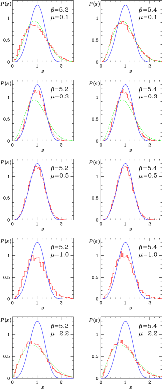
FIG. 3.: Nearest-neighbor spacing distribution of the Dirac operator eigenvalues in the complex plane for various values of $\mu$ in the confinement ($\beta=5.2$, left) and deconfinement ($\beta=5.4$, right) phase. The histograms represent the lattice data. The solid curve is the Ginibre distribution of Eq. (4), the short-dashed curve in the upper two rows the Wigner distribution of Eq. (3), and the dotted curve in the lowest row the Poisson distribution of Eq. (6), respectively.

Our results for $P(s)$ are shown in Fig. 3. There are minor quantitative but no qualitative differences between confinement and deconfinement phases, which is consistent with our findings at $\mu=0$ (second reference of [12]). As a function of $\mu$, we expect to find a transition from Wigner to Ginibre behavior in $P(s)$. This is indeed seen in the figures. For $\mu=0.1$, the data are still very close to the Wigner distribution of Eq. (3) whereas for $0.5\leq\mu\leq 0.7$ ($\mu=0.7$ not shown) we observe nice agreement with the Ginibre distribution of Eq. (4). Values of $\mu$ in the crossover region between Wigner and Ginibre behavior ($0.1<\mu<0.3$) correspond to the regime of weak non-Hermiticity mentioned above. In this regime, the derivation of the spacing distribution is a very difficult problem, and the only known analytical result is $P(s,z_{0})$ for small $s$, where $z_{0}$ is the location in the complex plane (i.e., no unfolding is performed) [7]. The small-$s$ behavior of Eqs. (3) and (4) is given by $P_{\rm W}(s)\propto s^{2}$ and $P_{\rm G}(s)\propto s^{3}$, respectively, and in the regime of weak non-Hermiticity we have $P(s,z_{0})\propto s^{\alpha}$ (for $s\ll 1$) with $2<\alpha<3$ [7]. This smooth crossover from $\alpha=2$ to $\alpha=3$ is also observed in our unfolded data.

For $\mu>0.7$ the lattice results for $P(s)$ deviate substantially from the Ginibre distribution. It is also evident from the appearance of the spectra for $\mu=1.0$ and 2.2 in Fig. 1 that the global spectral density of the lattice data is very different from that of the Ginibre ensemble. While this does not immediately imply that the local spectral fluctuations are also different, it is an indication for qualitative changes. In particular, the results for $\mu=2.2$ in Fig. 3 could be interpreted as Poisson behavior, corresponding to uncorrelated eigenvalues. In the Hermitian case at finite temperature, $T$, lattice simulations show a transition to Poisson behavior only for $\beta\to\infty$ when the physical box size shrinks and the theory becomes free [12]. Here, however, we have to remember that the chemical potential was neglected in the generation of the equilibrium gauge fields so that conclusions about the physical content of this observation should be drawn with care. Specifically, we are not entitled to make definite statements on possible connections between the finite-density phase transition (expected at smaller values of $\mu$) and the deviations from Ginibre behavior. A more plausible explanation of the transition to Poisson behavior is provided by the following two (related) observations. First, for large $\mu$ the terms containing $e^{\mu}$ in Eq. (2) dominate the Dirac matrix, giving rise to uncorrelated eigenvalues. Second, for $\mu>1.0$ the fermion density on the $6^{3}\times 4$ lattice reaches its maximum value given by the Pauli exclusion principle. In any event, the mechanisms behind this transition are interesting and deserve further study.

If a solution to the problem of the generation of configurations with a complex weight function becomes available, it would be very interesting to redo our analysis. Since previous computations in the deconfinement phase at $\mu=0$ have verified the RMT predictions [12], and since the present simulations at $\beta=5.4$ are already in the deconfinement phase for all values of $\mu$, we expect the observed Ginibre behavior to persist. Of course, this should be verified by a full finite-density simulation.

In conclusion, we have proposed a general unfolding procedure for the spectra of non-Hermitian operators. This procedure was applied to the QCD lattice Dirac operator at finite chemical potential. Agreement of the nearest-neighbor spacing distribution with predictions of the Ginibre ensemble of non-Hermitian RMT was found between $\mu=0.5$ and $\mu=0.7$ in both confinement and deconfinement phases. The deviations from Ginibre behavior for smaller values of $\mu$ are well understood whereas the deviations for larger values of $\mu$ toward a Poisson distribution require a better understanding of QCD at finite density. In this context, an interesting observation is that the results for $P(s)$ in the non-Hermitian case are rather sensitive to $\mu$ whereas they are very stable under variations of $T$ in the Hermitian case [12]. It would be interesting to apply our unfolding method to other non-Hermitian systems [4, 18].

This work was supported by FWF project P10468-PHY and DFG grant We 655/15-1. We thank N. Kaiser, K. Rabitsch, and J.J.M. Verbaarschot for discussions.

REFERENCES

- [1] R. Grobe, F. Haake, and H.-J. Sommers, Phys. Rev. Lett. 61, 1899 (1988).
- [2] N. Hatano and D. Nelson, Phys. Rev. Lett. 77, 570 (1996).
- [3] K.B. Efetov, Phys. Rev. Lett. 79, 491 (1997).
- [4] H.-J. Sommers, A. Crisanti, H. Sompolinsky, and Y. Stein, Phys. Rev. Lett. 60, 1895 (1988); N. Lehmann and H.-J. Sommers, Phys. Rev. Lett. 67, 941 (1991); B. Doyon, B. Cessac, M. Quoy, and M. Samuelidis, Int. J. Bifurc. Chaos 3, 279 (1993).
- [5] M.A. Stephanov, Phys. Rev. Lett. 76, 4472 (1996).
- [6] J. Ginibre, J. Math. Phys. 6, 440 (1965).
- [7] Y.V. Fyodorov and H.-J. Sommers, JETP Lett. 63, 1026 (1996), J. Math. Phys. 38, 1918 (1997); Y.V. Fyodorov, B.A. Khoruzhenko, and H.-J. Sommers, Phys. Lett. A 226, 46 (1997), Phys. Rev. Lett. 79, 557 (1997).
- [8] K.B. Efetov, Phys. Rev. B 56, 9630 (1997).
- [9] J. Feinberg and A. Zee, Nucl. Phys. B 504, 579 (1997).
- [10] R.A. Janik, M.A. Nowak, G. Papp, and I. Zahed, Nucl. Phys. B 501, 603 (1997).
- [11] T. Guhr, A. Müller-Groeling, and H.A. Weidenmüller, Phys. Rep. 299, 189 (1998) and references therein.
- [12] M.A. Halasz and J.J.M. Verbaarschot, Phys. Rev. Lett. 74, 3920 (1995); R. Pullirsch, K. Rabitsch, T. Wettig, and H. Markum, Phys. Lett. B 427, 119 (1998); B.A. Berg, H. Markum, and R. Pullirsch, Phys. Rev. D 59, 097504 (1999); R.G. Edwards, U.M. Heller, J. Kiskis, and R. Narayanan, Phys. Rev. Lett. 82, 4188 (1999).
- [13] P. Hasenfratz and F. Karsch, Phys. Lett. B 125, 308 (1983); I.M. Barbour, Nucl. Phys. B (Proc. Suppl.) 26, 22 (1992).
- [14] J.J.M. Verbaarschot, Phys. Rev. Lett. 72, 2531 (1994); M.A. Halasz, J.C. Osborn, and J.J.M. Verbaarschot, Phys. Rev. D 56, 7059 (1997).
- [15] I.M. Barbour, S.E. Morrison, E.G. Klepfish, J.B. Kogut, and M.P. Lombardo, Phys. Rev. D 56, 7063 (1997).
- [16] M.A. Halasz, A.D. Jackson, and J.J.M. Verbaarschot, Phys. Rev. D 56, 5140 (1997).
- [17] I. Barbour, N.-E. Behilil, E. Dagotto, F. Karsch, A. Moreo, M. Stone, and H.W. Wyld, Nucl. Phys. B 275, 296 (1986).
- [18] V.V. Sokolov and V.G. Zelevinsky, Phys. Lett. B 202, 10 (1988), Nucl. Phys. A 504, 562 (1989); F. Haake, F. Izrailev, N. Lehmann, D. Saher, and H.-J. Sommers, Z. Phys. B 88, 359 (1992); N. Lehmann, D. Saher, V.V. Sokolov, and H.-J. Sommers, Nucl. Phys. A 582, 223 (1995); M. Müller, F.-M. Dittes, W. Iskra, and I. Rotter, Phys. Rev. E 52, 5961 (1995).