UTHEP-404 UTCCP-P-66 June 1999 Two dimensional lattice Gross–Neveu model
with domain-wall fermions

Abstract

We investigate the two dimensional lattice Gross–Neveu model in large flavor number limit using the domain-wall fermion formulation, as a toy model of lattice QCD. We study nonperturbative behavior of the restoration of chiral symmetry of the domain-wall fermions as the extent of the extra dimension $(N_{s})$ is increased to infinity. We find the the parity broken phase (Aoki phase) for finite $N_{s}$, and study the phase diagram, which is related to the mechanism of the chiral restoration in $N_{s}\to\infty$ limit. The continuum limit is taken and $O(a)$ scaling violation of observables vanishes in $N_{s}\to\infty$ limit. We also examine the systematic dependencies of observables to the parameters.

I Introduction

Chiral symmetry is one of the important properties to understand the hadron physics and the phase transition in the thermodynamics of field theories. Pions are regarded as the pseudo Nambu-Goldstone bosons associated with the spontaneous breakdown of chiral symmetry. Physics of the phase transition between the confining phase (Hadron phase) and the deconfining phase (Quark-Gluon Plasma phase) in QCD is interested from the theoretical and experimental point of view. The lattice field theory is one of the most powerful tool for such important physics beyond perturbations.

However there is a problem to define chiral symmetry on a lattice. The definition of chiral symmetry on the lattice is one of long-standing problems of the lattice field theory. This problem is called as “no-go theorem” [1, 2]: the unwanted species of fermions appear in chiral symmetric theory on the lattice. To avoid this, chiral symmetry has to be broken by adding the Wilson term to the Lagrangian[3, 4]. This formulation is known as Wilson fermion (WF). In order to obtain the chiral symmetric theory in the continuum limit, one has to fine tune the quark mass parameter to cancel the additive quantum correction, which is a non trivial task in numerical simulations. Besides this fine tuning difficulty, the physical prediction from WF has $O(a)$ scaling violation due to the absence of chiral symmetry, where $a$ is the lattice spacing. One must calculate on a fine lattice to get precise predictions in WF.

Few years ago, the domain-wall fermion (DWF) is proposed [5, 6] as the new formulation of lattice fermion. DWF is formulated as $D+1$ dimensional Wilson fermion with the free boundary condition in the extra dimension [6]. When the extra dimension becomes infinite, DWF has a massless fermion with chiral symmetry. Because of this property, the current quark mass term in DWF receives multiplicative renormalization in contrast with WF, and this fermion formulation does not need the fine tuning in order to restore chiral symmetry on the lattice [7, 8]. The $O(a)$ scaling violation is expected to vanish in large $N_{s}$ limit, which means smaller scaling violations than in WF. Thus DWF has desirable property for defining the lattice fermion especially for chiral symmetric or near massless cases.

The numerical simulations of the domain-wall QCD (DWQCD) have been already carried out [9, 10]. As a trade off of the above ideal properties, one needs a large amounts of CPU time for computer simulations of DWQCD. Furthermore the new model has larger number of parameters than that of WF, and results of simulations have complicated dependencies to parameters.

To clarify the nonperturbative properties of DWF, we examine the formalism for the solvable theory, Gross-Neveu model (GN model) in two dimensions, which shares common natures with QCD. Our main purpose in this paper is to understand the restoration of chiral symmetry. For finite $N_{s}$, for which the lattice simulations are performed, we will see that chiral symmetry is broken, and the model can be seen as “improved Wilson fermion”. DWF for finite $N_{s}$ has the parity broken phase similar to WF[11, 12, 13]. We also study the continuum limit of DWF model. We will see the $O(a)$ becomes small as $N_{s}$ is increased and vanishes in the limit $N_{s}\to\infty$.

This paper is organized as follows: In Sec.II, after a brief review of the GN model in the continuum, the lattice GN model with DWF is formulated and the effective potentials in large flavor ($N$) limit are calculate when the extent of extra dimension $(N_{s})$ is both infinite and finite. In Sec.III we calculate the continuum limit in infinite and finite $N_{s}$ case and discuss the restoration of chiral symmetry. We will see that the model has chiral symmetry on the lattice for infinite $N_{s}$, while the symmetry is restored only in the continuum limit with fine tuning for finite $N_{s}$. In Sec.IV we analyze the structure of the chiral phase boundary between the parity symmetric and the parity broken phase (Aoki phase) for the finite lattice spacing by solving the gap equation and discuss the necessity of fine tuning to restore the chiral symmetry. In Sec.V we study the parameter dependences of the lattice observables and in Sec.VI we discuss the way of taking the continuum limit. We will see that the correct continuum limit are taken from the lattice model and $O(a)$ scaling violation vanishes for $N_{s}\to\infty$ limit. We conclude with a summary in Sec. VII.

II Action and The Effective Potential

A Continuum Gross–Neveu model

The investigation of the GN model is a good test [11, 14, 15, 16, 17] for the nonperturbative behavior of QCD since the two theories share common properties: the feature of asymptotic freedom, chiral symmetry and its spontaneous breakdown.

The two dimensional continuum Gross-Neveu model in Euclidean space is defined by the action

$$S=\int dx^{2}\{\bar{\psi}(\gamma_{\mu}\partial_{\mu}+m)\psi-{g^{2}\over 2N}[(\bar{\psi}\psi)^{2}+(\bar{\psi}i\gamma_{5}\psi)^{2}]\}~{},$$ (1)

where $\psi$ is an $N$-component fermion field. The effective potential in large $N$ limit in the continuum theory is given as

$$V_{eff}=-m\sigma+\frac{1}{4\pi}\left(\sigma^{2}+\Pi^{2}\right)\ln\frac{\sigma^{2}+\Pi^{2}}{e\Lambda^{2}}\,,$$ (2)

where $m$ is the renormalized mass and $\Lambda$ is the scale parameter. If the momentum integration is regularized by a cutoff, $M$, the renormalization for bare mass $m_{0}$ and the bare coupling constant $g^{2}$ are

$$m = {m_{0}\over g^{2}}~{},$$ (3)

$${1\over g^{2}} = {1\over 2\pi}\ln{M^{2}\over\Lambda^{2}}~{},$$ (4)

where the latter shows the asymptotically free. (We set the renormalized coupling constant to unity)

The auxiliary field $\sigma$ and $\Pi$ relate to the fermion condensations by equation of motion

$$\sigma=m_{0}-\frac{g^{2}}{N}\bar{\psi}\psi,~{}~{}~{}\Pi=\frac{g^{2}}{N}\bar{\psi}i\gamma_{5}\psi~{}.$$ (5)

When $m_{0}$ vanishes the model shows chiral symmetry, which is expressed by the $O(2)$ rotational invariance of effective action (2) in $(\sigma,\Pi)$ space. The stationary point of the effective action (2) satisfies $\sigma^{2}+\Pi^{2}=\Lambda^{2}$, which manifests the spontaneous breakdown of chiral symmetry.

B Lattice model with DWF

DWF is formulated as Wilson fermion (WF) in $D+1$ dimensions, or equivalently $N_{s}$ flavor WF with a flavor mixing, which has negative Wilson term obeying the free boundary condition on the edges in the extra dimension[6].

The action of DWF is given as follows:

$$S_{\rm free}=a^{2}\sum_{s,t}\sum_{m,n}\overline{\psi}(m,s)D^{free}(m,s;n,t)\psi(n,t),$$ (6)

where

$$D^{free}(m,s;n,t)=\sum_{\mu=1}^{2}\sigma_{\mu}C_{\mu}(m,n)\delta_{s,t}-W(m,n)\delta_{s,t}+P_{R}\delta_{s+1,t}\delta_{m,n}+P_{L}\delta_{s,t+1}\delta_{m,n},$$ (7)

$$C_{\mu}(m,n)=\frac{a_{s}}{2a}\left[\delta_{m+\hat{\mu},n}-\delta_{m-\hat{\mu},n}\right],$$ (8)

$$W(m,n)=(1-M)\delta_{m,n}+\frac{ra_{s}}{2a}\left[2\delta_{m,n}-\delta_{m+\hat{\mu},n}-\delta_{m,n+\hat{\mu}}\right]\,.$$ (9)

$P_{R/L}=(1\pm\gamma_{5})/2$ are the projection operators into the right- and the left-handed mode, $a$ and $a_{s}$ are the lattice spacing in two dimensions and the third dimensions respectively. $\sigma_{\mu}$’s are defined as $\sigma_{1}=i$ and $\sigma_{2}=1$ in two dimensions, $s$ and $t$ are the indecies of extra dimension with $1\leq s,t\leq N_{s}$. Here, $r(>0)$ is Wilson coupling constant and $M$ is the domain-wall mass height (DW-mass). The boundary condition in the third direction takes the free boundary condition. In the followings, we take $a=a_{s}$ and $r=1$ for simplicity.

If one sets $0<M<2$, there is single light Dirac fermion in the spectrum of this free action whose right(left)-handed components stays near $s=1(N_{s})$,

$$q(n)=P_{R}\psi(n,s=1)+P_{L}\psi(n,s=N_{s})~{}.$$ (10)

The mass of this light quark, $q(n)$, is exponentially suppressed for large $N_{s}$,

$$m_{q}a\sim(1-M)^{N_{s}}~{}.$$ (11)

Wilson term in the action avoids the species doubling problem. The doublers and other $N_{s}-1$ bulk fermions acquire the cut-off order mass and decouple from low energy physics.

As a toy model of the lattice DWQCD, we define the two dimensional lattice GN model with $N$ flavors:

$$S=S_{free}+a^{2}\sum_{n}am_{f}\bar{q}(n)q(n)-a^{2}\sum_{n}\left[\frac{g_{\sigma}^{2}}{2N}\left\{\bar{q}(n)q(n)\right\}^{2}+\frac{g_{\pi}^{2}}{2N}\left\{\bar{q}(n)i\gamma_{5}q(n)\right\}^{2}\right]~{},$$ (12)

where we abbreviate $\overline{\psi}(n,s)\psi(n,t)=\sum_{i=1}^{N}\overline{\psi}^{i}(n,s)\psi^{i}(n,t)$. $m_{f}$ is the “current quark mass” in order to give the mass to the fermion. In perturbation of DWQCD, $m_{f}$ receives the multiplicative renormalization in $N_{s}\to\infty$ case[7, 8]. DW-mass $M$, on the other hand, receives the additive renormalization[7, 8], because $M$ corresponds to Wilson mass term. We will see that two different couplings, $g^{2}_{\sigma}$ and $g^{2}_{\pi}$, are needed for chiral symmetry in general.

The action (12) can be rewritten into the following equivalent action using the auxiliary fields $\sigma(n)$ and $\Pi(n)$:

$$S = S_{\rm free}+a^{2}\sum_{n}\bar{q}(n)\left\{a\sigma(n)+i\gamma_{5}a\Pi(n)\right\}q(n)$$ (13)

$$+ \quad a^{2}\sum_{n}\left[\frac{N}{2g_{\sigma}^{2}}\left\{\sigma(n)-m_{f}\right\}^{2}+\frac{N}{2g_{\pi}^{2}}\Pi(n)^{2}\right]~{}.$$ (14)

The auxiliary fields are related to condensations of fermion;

$$\sigma(n)=m_{f}-\frac{g_{\sigma}^{2}}{N}\bar{q}(n)q(n)\quad,\quad\Pi(n)=-\frac{g_{\pi}^{2}}{N}\bar{q}(n)i\gamma_{5}q(n)\,.$$ (15)

from the equations of motion.

C the effective potential

We calculate the effective potential of the two dimensional lattice GN model in large $N$ limit. In large $N$ limit, in which the quantum fluctuation of $\sigma(n)$ and $\Pi(n)$ is suppressed and the mean field approximation, $\sigma(n)\to\sigma$ and $\Pi(n)\to\Pi$, becomes exact. the effective potential of GN model is obtained by exponentiating the fermion determinant which is calculated by the integration of the fermion fields $\psi$:

$$Z = \int[d\psi][d\overline{\psi}]e^{-a^{2}\sum\overline{\psi}D\psi}e^{-a^{2}\sum[\frac{N}{2g_{\sigma}^{2}}(\sigma-m_{f})^{2}+\frac{N}{2g_{\pi}^{2}}\Pi^{2}]}$$ (16)

$$= \det D(\sigma,\Pi)\,e^{-a^{2}\sum[\frac{N}{2g_{\sigma}^{2}}(\sigma-m_{f})^{2}+\frac{N}{2g_{\pi}^{2}}\Pi^{2}]}=e^{-a^{2}V_{eff}}\,.$$ (17)

This determinant can be calculated by employing the technique of the propagator matrix [19, 20]. The action introduced in the previous subsection is rewritten by the matrix representation, in the momentum space. From (14),

$$S=\bar{\psi}D(\sigma,\Pi)\psi=a^{2}\sum_{s,t}\sum_{m,n}\left(\psi^{{\dagger}}_{L}(m,s),\psi^{{\dagger}}_{R}(m,s)\right)\left[\left(\begin{array}[]{cc}C^{{\dagger}}&-W\\ -W&-C\end{array}\right)\delta_{s,t}+\left(\begin{array}[]{cc}0&0\\ 1&0\end{array}\right)\delta_{t,s+1}\right.$$ (22)

$$\left.+\left(\begin{array}[]{cc}0&1\\ 0&0\end{array}\right)\delta_{s,t+1}+\left(\begin{array}[]{cc}0&0\\ a\omega&0\end{array}\right)\delta_{s,N}\delta_{t,1}+\left(\begin{array}[]{cc}0&a\omega^{{\dagger}}\\ 0&0\end{array}\right)\delta_{s,1}\delta_{t,N_{s}}\right]\left(\begin{array}[]{c}\psi_{L}(n,t)\\ \psi_{R}(n,t)\end{array}\right)\,,$$ (31)

where $C^{{\dagger}}=\sin(p_{1}a)+i\sin(p_{2}a)$, $\omega=\sigma+i\Pi$ and $W=(1-M)+\sum_{\mu=1}^{2}[1-\cos(p_{\mu}a)]$. After some calculations similar to Ref.[19, 20], we have

$$\det D(\sigma,\Pi)=\det\left[\left(\begin{array}[]{cc}a\omega&0\\ 0&1\end{array}\right)-T^{-N_{s}}\left(\begin{array}[]{cc}1&0\\ 0&a\omega^{{\dagger}}\end{array}\right)\right]\,,$$ (32)

where $T$ is the transfer matrix along the extra dimension defined by

$$T=e^{a_{s}H_{s}}=\left(\begin{array}[]{ccc}\frac{\displaystyle{1}}{\displaystyle{W}}&,&-\frac{\displaystyle{1}}{\displaystyle{W}}C\\ -C^{{\dagger}}\frac{\displaystyle{1}}{\displaystyle{W}}&,&W+C^{{\dagger}}\frac{\displaystyle{1}}{\displaystyle{W}}C\end{array}\right)\quad,\quad T^{-1}=\left(\begin{array}[]{ccc}C^{{\dagger}}\frac{\displaystyle{1}}{\displaystyle{W}}C+W&,&C\frac{\displaystyle{1}}{\displaystyle{W}}\\ \frac{\displaystyle{1}}{\displaystyle{W}}C^{{\dagger}}&,&\frac{\displaystyle{1}}{\displaystyle{W}}\end{array}\right)\,.$$ (33)

$H_{s}$ is the Hamiltonian along to the extra dimension. The overall factor in Eq. (32) is omitted. Diagonalized $T^{-1}$, whose eigenvalues are $\lambda$ and $1/\lambda$, we obtain a explicit formula for the determinant,

$$\det D(\sigma,\Pi)=\prod_{p_{\mu}}\left[F(M,N_{s},p_{\mu})a^{2}(\sigma^{2}+\Pi^{2})+G(M,N_{s},p_{\mu})a\sigma+H(M,N_{s},p_{\mu})\right]\,,$$ (34)

where

$$H(M,N_{s},p_{\mu})=\frac{-1}{2f}\left[-(\lambda^{N_{s}}-\lambda^{-N_{s}})(2-h)+(\lambda^{N_{s}}+\lambda^{-N_{s}})f\right]\,,$$ (35)

$$F(M,N_{s},p_{\mu})=\frac{-1}{2f}\left[(\lambda^{N_{s}}-\lambda^{-N_{s}})(2-h)+(\lambda^{N_{s}}+\lambda^{-N_{s}})f\right]\,,$$ (36)

$$G(M,N_{s},p_{\mu})=\frac{-1}{2f}\left[-4f\right]=2\,,$$ (37)

$$h=1+W^{2}+\bar{p}^{2}\quad,\quad f=\sqrt{-4W^{2}+h^{2}},$$ (38)

$$\lambda\,=\frac{1}{2W}\left[h+f\right]\,\,(\left|\lambda\right|>1)\quad,\quad\frac{1}{\lambda}=\frac{1}{2W}\left[h-f\right]\,\,(\left|\lambda\right|<1)\,,$$ (39)

$$W=(1-M)+\sum_{\mu=1}^{2}\left[1-\cos(p_{\mu}a)\right]\quad,\quad\bar{p}^{2}=\sin^{2}(p_{1}a)+\sin^{2}(p_{2}a)\,.$$ (40)

Substituting (34) into (17), we obtain the effective potential of the two dimensional lattice GN model in the large $N$ limit:

$$V_{eff}=\frac{1}{2g_{\sigma}^{2}}\left(\sigma-m_{f}\right)^{2}+\frac{1}{2g_{\pi}^{2}}\Pi^{2}-I(\sigma,\Pi,M,N_{s})$$ (41)

$$I(\sigma,\Pi,M,N_{s})=\int_{-\pi/a}^{\pi/a}\frac{d^{2}p}{(2\pi)^{2}}\ln\left[Fa^{2}(\sigma^{2}+\Pi^{2})+Ga\sigma+H\right].$$ (42)

This effective potential is symmetric under $M\rightarrow 6-M$.

Here we comment about the absence of the bosonic fields (Pauli-Villars fields) in our model which is employed in (full) QCD[7, 9, 10]. Since the gauge field in QCD equally interacts with not only light quark field, $q(n)$, but also heavy (bulk) fermions $\psi(n,s)$, one should introduce the Pauli-Villars boson to subtract this heavy fermion effects. In GN model $\sigma$ and $\Pi$ play analogous role to the gauge field in full QCD except that they couples with $q(n)$ only. Thus it is not necessary to introduce the subtraction in our model. One the other hand one could think about a new four Fermi interaction model, in which whole $\psi(n,s),s=1,\cdots,N_{s}$ equally couple to auxiliary fields, $\sigma$ and $\Pi$. However these fields are constituted from both light and heavy fermions and don’t show the chiral property in such a new model.

III Chiral symmetry restoration

First we show how chiral symmetry restores in this model in the case of both $N_{s}=\infty$ and $N_{s}<\infty$ by examining the effective potential given in previous section.

We will see that for infinite $N_{s}$ case chiral symmetry is exact even for finite lattice spacing, $a>0$, without fine tuning for bare mass parameters. The situation for finite $N_{s}$ case, on the other hand, is much like that of Wilson fermion action. The continuum limit has to be taken, and at same time, the bare mass parameter must be tuned finely for chiral symmetric effective potential for $N_{s}<\infty$.

A The effective potential in “$N_{s}=\infty$” case

In this subsection we calculate the expression of the effective potential for $N_{s}=\infty$ case.

For large $N_{s}$, one easily sees that the dominant contributions for function $I(\sigma,\Pi)$ in the effective potential (42) are the functions “$F$” and “$H$”, which behave as $\lambda^{N_{s}}$ in $N_{s}\rightarrow\infty$ limit, from Eqs. (35) and (36). The chiral breaking term “$Ga\sigma$” in (42) can be ignore in the limit $N_{s}\to\infty$ and (42) could be written as

$$I(\sigma,\Pi)=\int_{-\pi/a}^{\pi/a}\frac{d^{2}p}{(2\pi)^{2}}\ln\left[H+Fa^{2}(\sigma^{2}+\Pi^{2})\right].$$ (43)

So the effective potential (41) is a function of $\sigma^{2}+\Pi^{2}$, which is invariant under the $O(2)$ rotation if $g_{\sigma}^{2}=g_{\pi}^{2}$. We emphasize that this is chiral symmetry even before taking the continuum limit, $a\to 0$.

The continuum limit of the effective potential can be evaluated by separating divergent parts and finite parts from (43). Rewriting (43) into a integration form

$$I(\sigma,\Pi)=\int_{0}^{\sigma^{2}+\Pi^{2}}d\rho K(\rho)\quad,\quad K(\rho)=\int_{-\pi/a}^{\pi/a}\frac{d^{2}p}{(2\pi)^{2}}\frac{1}{\frac{\displaystyle{H}}{\displaystyle{Fa^{2}}}+\rho}\,,$$ (44)

one can pick up the the divergent part in $a\to 0$, near zero fermion momentum, $p_{\mu}a=(0,0)$, for $\rho a^{2}\sim 0$. Since the divergent part of $K(\rho)$ behaves as

$$\frac{H}{Fa^{2}}\rightarrow\frac{1}{M^{2}(2-M)^{2}}\sum_{\mu=1}^{2}p_{\mu}^{2}\,,$$ (45)

in $a\to 0$ limit, the function $K(\rho)$ becomes

$$K(\rho)=\int_{-\pi/a}^{\pi/a}\frac{d^{2}p}{(2\pi)^{2}}\frac{1}{f_{M}^{-2}\sum_{\mu=1}^{2}p_{\mu}^{2}+\rho}+C_{0}(M,N_{s})\,,$$ (46)

where $f_{M}=M(2-M)$ and

$$C_{0}(M,N_{s})=\int_{-\pi}^{\pi}\frac{d^{2}\xi}{(2\pi)^{2}}\frac{f_{M}^{-2}\sum_{\mu}\xi_{\mu}^{2}-\frac{\displaystyle{H}}{\displaystyle{F}}}{\frac{\displaystyle{H}}{\displaystyle{F}}f_{M}^{-2}\sum_{\mu}\xi_{\mu}^{2}}\,,$$ (47)

with $\xi_{\mu}=p_{\mu}a$. The factor $f_{M}$ appears as the normalization factor of the propagator: $\langle q\bar{q}\rangle\sim f_{M}(ip_{\mu}\gamma_{\mu})^{-1}$. The wavefunction of the massless eigenmode has finite width in the $s$ direction, and $f_{M}$ is the ratio of $q(n)$ to the the zero mode.

In $N_{s}=\infty$ case, when $0<M<2$, only the momentum around $p_{\mu}a=(0,0)$ dominates in (43) and the contributions of doublers, $p_{\mu}a=(\pi,0),(0,\pi)$ and $(\pi,\pi)$, are removed completely. This means that the doublers decouple from the physical spectrum. For $2<M<4$ the momenta $p_{\mu}a=(\pi,0)$ and $(0,\pi)$ become physical poles in the momentum integral, while the remaining mode at $p_{\mu}a=(\pi,\pi)$ is dominant for $4<M<6$. In these two regions of $M$, the normalization factor $f_{M}$ becomes $(M-2)(4-M)$ and $(M-4)(6-M)$ respectively. For $M<0$ and $M>6$, the no physical pole emerges.

By evaluation of the first term in the right hand side in Eq. (46), we find

$$K(\rho)=\frac{f_{M}^{2}}{4\pi}\ln\frac{1}{a^{2}f_{M}^{2}\rho}+\hat{C_{0}}(M,N_{s}),$$ (48)

where the new constant $\hat{C_{0}}$ is defined by $\hat{C_{0}}=C_{0}+C_{0}^{\prime}$ with

$$\int_{-\pi/a}^{\pi/a}\frac{d^{2}p}{(2\pi)^{2}}\frac{1}{f_{M}^{-2}\sum_{\mu=1}^{2}p_{\mu}^{2}+\rho}\equiv\frac{f_{M}^{2}}{4\pi}\ln\frac{1}{a^{2}f_{M}^{2}\rho}+C_{0}^{\prime}(M,N_{s}).$$ (49)

By substituting this expression into Eq. (44), we obtain

$$I=-\frac{f_{M}^{2}}{4\pi}\left(\sigma^{2}+\Pi^{2}\right)\ln\frac{a^{2}f_{M}^{2}\left(\sigma^{2}+\Pi^{2}\right)}{e}+\hat{C_{0}}\left(\sigma^{2}+\Pi^{2}\right).$$ (50)

Therefore the continuum limit of the effective potential for $N_{s}=\infty$ case is

$$V_{eff}=-\frac{m_{f}}{g^{2}}\sigma+\left(\frac{1}{2g^{2}}-\hat{C_{0}}+\frac{f_{M}^{2}}{4\pi}\ln a^{2}\right)\left(\sigma^{2}+\Pi^{2}\right)+\frac{f_{M}^{2}}{4\pi}\left(\sigma^{2}+\Pi^{2}\right)\ln\frac{f_{M}^{2}\left(\sigma^{2}+\Pi^{2}\right)}{e}.$$ (51)

We find that the two coupling constants can be same as each other $g^{2}=g_{\sigma}^{2}=g_{\pi}^{2}$ from above result, which is in contrast to the GN model with WF. As mentioned above, since the effective potential has chiral symmetry for finite lattice spacing, the fine tuning is unnecessary for chiral symmetric continuum limit.

After redefining for $\sigma$ and $\Pi$ such as $\sigma_{R}=f_{M}\sigma$ and $\Pi_{R}=f_{M}\Pi$, we renormalize the coupling constant $g$ and $m_{f}$ as follows:

$$\frac{1}{2g^{2}}=\hat{C_{0}}+\frac{f_{M}^{2}}{4\pi}\ln\frac{1}{a^{2}\Lambda^{2}}\,,$$ (52)

$$m=\frac{m_{f}}{f_{M}g^{2}}=m_{f}\left(\frac{2}{f_{M}}\hat{C_{0}}+\frac{f_{M}}{2\pi}\ln\frac{1}{a^{2}\Lambda^{2}}\right)\,,$$ (53)

where $\Lambda$ is the scale parameter and $m$ is the renormalized mass parameter. One realizes that the current quark mass term, $m_{f}$, receives the multiplicative renormalization (53), similar to the perturbation theory in infinitely large $N_{s}$. With this choice of scaling relations the continuum limit of the effective potential for $N_{s}=\infty$ is finally given as

$$V_{eff}=-m\sigma_{R}+\frac{1}{4\pi}\left(\sigma_{R}^{2}+\Pi_{R}^{2}\right)\ln\frac{\sigma_{R}^{2}+\Pi_{R}^{2}}{e\Lambda^{2}},$$ (54)

which is identical with the continuum theory (2).

B Chiral restoration in the continuum limit ($N_{s}$ finite case)

As we have seen in previous subsection, the limit $N_{s}\to\infty$ guarantees chiral symmetry on a lattice. Nevertheless, to understand the behavior of finite $N_{s}$ theory is important for lattice QCD simulations using DWF.

Let us start the finite $N_{s}$ analysis with the effective potential (41). The chiral breaking term, $Ga\sigma$, in (42) has the important role for finite $N_{s}$ and the GN model does not have chiral symmetry any more. Chiral symmetry can be restored in the continuum limit with fine tuning. In this sense, finite $N_{s}$ model is similar to WF. In order to restore the chiral symmetry without fine tuning, one should take the limit $N_{s}\to\infty$ before taking the continuum limit to obtain chiral symmetry on lattice.

The continuum limit for finite $N_{s}$ can be taken following the same procedures in the previous subsection. The difference from the calculation in $N_{s}\to\infty$ is a necessity to shift the auxiliary field:

$$\sigma^{\prime}=\sigma-\frac{\displaystyle{(1-M)^{N_{s}}}}{\displaystyle{a}}~{}.$$ (55)

The effective potential becomes as follows:

$$V_{eff}=\frac{1}{2g_{\sigma}^{2}}\left\{\sigma^{\prime}-\left(m_{f}-\frac{(1-M)^{N_{s}}}{a}\right)\right\}^{2}+\frac{1}{2g_{\pi}^{2}}\Pi^{2}-I(\sigma,\Pi)~{},$$ (56)

$$I(\sigma,\Pi)=\int_{-\pi/a}^{\pi/a}\frac{d^{2}p}{(2\pi)^{2}}\ln\left[H^{\prime}+Fa^{2}({\sigma^{\prime}}^{2}+\Pi^{2})+G^{\prime}a\sigma^{\prime}\right],$$ (57)

where

$$H^{\prime}=H+F(1-M)^{2N_{s}}+G(1-M)^{N_{s}}\quad,\quad G^{\prime}=G+2F(1-M)^{N_{s}}\,.$$ (58)

Expanding $I(\sigma,\Pi)$ into a power series of lattice spacing:

$$I=I_{0}+I_{1}+I_{2}+\cdots$$ (59)

$$I_{0}=\int_{-\pi/a}^{\pi/a}\frac{d^{2}p}{(2\pi)^{2}}\ln\left[H^{\prime}+Fa^{2}({\sigma^{\prime}}^{2}+\Pi^{2})\right],$$ (60)

$$I_{n}=-\frac{(-1)^{n}}{n}\int_{-\pi/a}^{\pi/a}\frac{d^{2}p}{(2\pi)^{2}}\left[\frac{G^{\prime}a\sigma^{\prime}}{H^{\prime}+Fa^{2}({\sigma^{\prime}}^{2}+\Pi^{2})}\right]^{n}.\quad(n\geq 1)$$ (61)

One can see that $I_{0}$ preserve $O(2)$ rotation in $(\sigma^{\prime},\Pi)$ plane, while $I_{n}(n\geq 1)$ break it.

$I_{0}$ is calculated in the same way as in $N_{s}=\infty$ case:

$$I_{0}=\int_{0}^{{\sigma^{\prime}}^{2}+\Pi^{2}}d\rho K(\rho)\quad,\quad K(\rho)=\int_{-\pi/a}^{\pi/a}\frac{d^{2}p}{(2\pi)^{2}}\frac{1}{\frac{\displaystyle{H^{\prime}}}{\displaystyle{Fa^{2}}}+\rho}\,.$$ (62)

Here we take the divergent part in $a\rightarrow 0$. The shifted function $H^{\prime}$ has similar behavior to the limit $N_{s}\to\infty$:

$$\frac{H^{\prime}}{Fa^{2}}\rightarrow f_{M}^{-2}\sum_{\mu}p_{\mu}^{2},$$ (63)

with

$$f_{M}=\frac{M(2-M)}{1-(1-M)^{2N_{s}}}\,.$$ (64)

Therefore the logarithmic divergent term has similar form as continuum theory:

$$I_{0}=-\frac{f_{M}^{2}}{4\pi}\left({\sigma^{\prime}}^{2}+\Pi^{2}\right)\ln\frac{a^{2}f_{M}^{2}\left({\sigma^{\prime}}^{2}+\Pi^{2}\right)}{e}+\hat{C_{0}}\left({\sigma^{\prime}}^{2}+\Pi^{2}\right),$$ (65)

where the new constant $\hat{C_{0}}$ is defined by $\hat{C_{0}}=C_{0}+C_{0}^{\prime}$ with

$$C_{0}(M,N_{s})=\int_{-\pi}^{\pi}\frac{d^{2}\xi}{(2\pi)^{2}}\frac{f_{M}^{-2}\sum_{\mu}\xi_{\mu}^{2}-\frac{\displaystyle{H^{\prime}}}{\displaystyle{F}}}{\frac{\displaystyle{H^{\prime}}}{\displaystyle{F}}f_{M}^{-2}\sum_{\mu}\xi_{\mu}^{2}}\,.$$ (66)

and

$$\int_{-\pi/a}^{\pi/a}\frac{d^{2}p}{(2\pi)^{2}}\frac{1}{f_{M}^{-2}\sum_{\mu=1}^{2}p_{\mu}^{2}+\rho}\equiv\frac{f_{M}^{2}}{4\pi}\ln\frac{1}{a^{2}f_{M}^{2}\rho}+C_{0}^{\prime}.(M,N_{s})~{}.$$ (67)

The coefficient $\hat{C}_{0}$ as a function of $M$ for various $N_{s}$ is plotted in Fig.1.

Remaining $I_{n}$ in the continuum limit is easily calculated. $I_{1}$ ($I_{2}$) is a linear divergent (constant) term in $a\to 0$ limit, while $I_{n}$ ($n\geq 3$) vanishes:

$$I_{1}=\frac{\sigma^{\prime}}{a}C_{1}=\frac{\sigma^{\prime}}{a}\int_{-\pi}^{\pi}\frac{d^{2}\xi}{(2\pi)^{2}}\frac{G^{\prime}}{H^{\prime}}\,,$$ (68)

$$I_{2}=-{\sigma^{\prime}}^{2}C_{2}=-{\sigma^{\prime}}^{2}\frac{1}{2}\int_{-\pi}^{\pi}\frac{d^{2}\xi}{(2\pi)^{2}}\left[\frac{G^{\prime}}{H^{\prime}}\right]^{2}\,.$$ (69)

Fig.2 shows these coefficients as a function of $N_{s}$ for various $M$.

From above calculations, the effective potential in finite $N_{s}$ case in the continuum limit is obtained as follows:

$$V_{eff} = -\left(\frac{m_{f}^{\prime}}{g_{\sigma}^{2}}+\frac{C_{1}}{a}\right)\frac{1}{f_{M}}\sigma_{R}+\left(\frac{1}{2g_{\sigma}^{2}}-\hat{C_{0}}+C_{2}\right)\frac{1}{f_{M}^{2}}\sigma_{R}^{2}$$ (70)

$$+ \left(\frac{1}{2g_{\pi}^{2}}-\hat{C_{0}}\right)\frac{1}{f_{M}^{2}}\Pi_{R}^{2}+\frac{1}{4\pi}\left(\sigma_{R}^{2}+\Pi_{R}^{2}\right)\ln\frac{a^{2}\left(\sigma_{R}^{2}+\Pi_{R}^{2}\right)}{e},$$ (71)

where

$$m_{f}^{\prime}=m_{f}-\frac{(1-M)^{N_{s}}}{a}\quad,\quad\sigma_{R}=f_{M}\sigma^{\prime}\quad,\quad\Pi_{R}=f_{M}\Pi\,.$$ (72)

If the coupling constants and the mass parameter are renormalized as

$$\frac{1}{2g_{\sigma}^{2}}-\hat{C_{0}}+C_{2}=\frac{f_{M}^{2}}{4\pi}\ln\frac{1}{a^{2}\Lambda^{2}},$$ (73)

$$\frac{1}{2g_{\pi}^{2}}-\hat{C_{0}}=\frac{f_{M}^{2}}{4\pi}\ln\frac{1}{a^{2}\Lambda^{2}},$$ (74)

$$\frac{1}{f_{M}}\left(\frac{m_{f}^{\prime}}{g_{\sigma}^{2}}+\frac{C_{1}}{a}\right)=m~{},$$ (75)

we obtain the correct effective potential of the continuum theory (2).

We emphasize that the current quark mass term, $m_{f}$, receives the $O(1/a)$ additive renormalization for $N_{s}=$ finite case. As we describe previously, fine tuning for bare mass parameter in (75) is needed for finite $N_{s}$, and chiral symmetry is restored in the continuum limit.

The restoration of chiral symmetry in $N_{s}\to\infty$ could also be seen in the scaling relation (73-75). The coefficients $C_{1}$ and $C_{2}$ represent the magnitudes of the explicit breaking of chiral symmetry. $C_{1}$ is the additive mass counter term, while $C_{2}$ is the miss match between the quadratic terms of scalar and pseudo scalar particle by the quantum correction. If we restrict DW-mass to $0<M<2$, as shown in Fig.2, the coefficients $C_{1}$ and $C_{2}$ are decreased rapidly as $N_{s}$ becomes large. The effects of shifting of the fields and the additive renormalization of the mass parameter in (72) and (75) rapidly vanishes with increasing $N_{s}$, thus the necessity of fine tuning becomes absent in $N_{s}\to\infty$ limit.

On the other hand, even when $M$ is set out of the region $(0,2)$, the scaling relations (73-75) lead the chiral symmetric continuum limit. In this case $C_{1}$ and $C_{2}$ don’t vanish in large $N_{s}$ limit and the fine tuning is necessary, similar to WF.

IV The parity broken phase and the restoration of chiral symmetry

For lattice QCD with WF, the existence of massless pion for finite lattice spacing is explained by the parity broken phase picture proposed by Aoki [11]. Although chiral symmetry is explicitly broken in WF, one can tune the mass parameter to obtain an exact massless pion in the spectrum even for finite lattice spacing. This cannot be understood by the ordinary picture of Nambu-Goldstone boson in the continuum theory, in which chiral symmetry is the exact symmetry of the action and is broken spontaneously.

Aoki examined the GN model and lattice QCD with WF for a finite lattice spacing, and found that the parity symmetric phase and parity(–flavor) spontaneously broken phase coexist in the parameter space of the model. The parity broken phase is characterized by the non-zero condensation of the pseudo scalar density, $\langle\Pi\rangle=\langle\psi i\gamma_{5}\psi\rangle\neq 0$. Provided a second-order phase transition separating the two phases from each other, pion becomes massless at the phase transition point, which is regarded as a massless particle accompanying with the continuous phase transition.

Before starting analysis of phase diagram of DWF model for general $N_{s}$, we note the equivalence between $N_{s}=1$ DWF model and Wilson fermion formalism. The effective potential of WF,

$$V_{\rm W}=\frac{1}{2g_{\sigma}^{2}}\left(\sigma-m_{f}\right)^{2}+\frac{1}{2g_{\pi}^{2}}\Pi^{2}$$ (76)

$$-\int_{-\pi/a}^{\pi/a}\frac{d^{2}k}{(2\pi)^{2}}\ln\left[\sum_{\mu}\frac{\sin^{2}k_{\mu}a}{a^{2}}+\left(\sigma_{c}+\frac{r}{a}\sum_{\mu}(1-\cos k_{\mu}a)\right)^{2}+\Pi_{c}^{2}\right]\,,$$ (77)

can be seen easily by substituting $N_{s}=1,\sigma_{c}=\sigma-(1-M)$ in (41). The phase boundary of Aoki phase forms the three cusps which reach the weak-coupling limit $g^{2}=0$ at $M=1,3,5$ in WF[11, 12, 13] and $N_{s}=1$ DWF model. Three cusps arise from the fact that the doublers at the conventional continuum limit, $(g^{2},M)=(0,1)$, become physical massless modes at at $M=3,5$.

On the other hand, in $N_{s}=\infty$ limit, the parity broken phase does not exist because of the restoration of chiral symmetry, whose explicit breaking causes the parity broken phase.

For $1<N_{s}<\infty$, it is expected that the parity broken phase exists and the chiral phase boundary forms the cusps as surmised from the Wilson like behavior in the previous section. The region of the broken phase is distorted and shrinks rapidly as $N_{s}$ is increased, and vanishes in $N_{s}\to\infty$ limit.

The parity symmetry is spontaneously broken at parameter point $(m_{f},g^{2};M,N_{s})$, where the gap equations have a stable solution $\Pi\neq 0$. Setting the parameters of this model $(m_{f},g_{\sigma}^{2},g_{\pi}^{2},M,N_{s})$ , observables are calculated by solving gap equations,

$$\frac{\partial V_{eff}}{\partial\sigma}=\frac{1}{g_{\sigma}^{2}}\left(\sigma-m_{f}\right)-\sigma{\cal{F}}(\sigma,\Pi)-{1\over a}{\cal{G}}(\sigma,\Pi)=0\,,$$ (78)

$$\frac{\partial V_{eff}}{\partial\Pi}=\Pi\left[\frac{1}{g_{\pi}^{2}}-{\cal{F}}(\sigma,\Pi)\right]=0\,,$$ (79)

where

$${\cal{F}}(\sigma,\Pi)=\int_{-\pi}^{\pi}\frac{d^{2}\xi}{(2\pi)^{2}}\frac{2F}{H+Ga\sigma+Fa^{2}(\sigma^{2}+\Pi^{2})}\,,$$ (80)

$${\cal{G}}(\sigma,\Pi)=\int_{-\pi}^{\pi}\frac{d^{2}\xi}{(2\pi)^{2}}\frac{G}{H+Ga\sigma+Fa^{2}(\sigma^{2}+\Pi^{2})}\,,$$ (81)

with $\xi_{\mu}=p_{\mu}a$. In the case of $g_{\pi}^{2}=g_{\sigma}^{2}=g^{2}$, the position of the phase boundary in the parameter space could be obtained by solving these gap equations for $\Pi=\epsilon$. Taking $\epsilon\to 0$ limit, (78) (79) define $g^{2}$ and $m_{f}$ as functions of $\sigma$ which is nothing but the parametric representation of the phase boundary if the phase transition is continuous.

Let us note that DWGN model with $g^{2}=g_{\sigma}^{2}=g_{\pi}^{2}$ has only second order phase transition between the parity symmetric and the broken phases. This is in contrast with WF case [17], in which theory a first order phase transition for $g_{\sigma}^{2}\neq g_{\pi}^{2}$ is found.

By differentiating (79) with respect to $\Pi$, one can easily check from that pion mass squared

$$M_{\pi}^{2}\propto\widetilde{M}_{\pi}^{2}\equiv{1\over f_{M}^{2}}{\partial^{2}V_{eff}(\sigma,\Pi=0)\over\partial\Pi^{2}}={1\over f_{M}^{2}}\left[{1\over g^{2}}-{\cal F}(\sigma,\Pi=0)\right]~{},$$ (82)

exactly vanishes at the phase boundary. The factor, $1/f_{M}^{2}$, in front of the r.h.s corrects the normalization of auxiliary field $\Pi$ in the same sense as explained in the previous section. (See below (47).)

Before drawing whole phase diagrams in the parameter space $(m_{f},g^{2})$, let us first examine the positions of the three “tips of cusps”, which are the intersection points between $g^{2}=0$ plane and the critical line. These tips correspond to the continuum limits $g^{2}\to 0$ similar to WF. The positions can be obtained by the asymptotic form of the integrals in (78) and (79). The divergent behaviors of the integrals around $p_{\mu}a=(\pi m,\pi n)$, with $m,n=0\,\,\,\mbox{or}\,\,\,1$, are

$${\cal{F}}(\sigma,\Pi=0) \rightarrow \sum_{m,n=0,1,l=m+n}\int_{-\pi}^{\pi}\frac{d^{2}\xi}{(2\pi)^{2}}\frac{2}{\left\{\sigma-(1-M+2l)^{N_{s}}\right\}^{2}+\sum_{\mu}{\cal{A_{\mu}}}\xi_{\mu}^{2}}\,,$$ (83)

$${\cal{G}}(\sigma,\Pi=0) \rightarrow \sum_{m,n=0,1,l=m+n}\int_{-\pi}^{\pi}\frac{d^{2}\xi}{(2\pi)^{2}}\frac{-2(1-M+2l)^{N_{s}}}{\left\{\sigma-(1-M+2l)^{N_{s}}\right\}^{2}+\sum_{\mu}{\cal{B_{\mu}}}\xi_{\mu}^{2}}\,,$$ (84)

where ${\cal{A_{\mu}}}$ and ${\cal{B_{\mu}}}$ are functions of $l,\sigma,M$ and $N_{s}$. From these expressions it is easy to see that the r.h.s of the gap equations (78) (79) have a logarithmic divergence at $\sigma=(1-M+2l)^{N_{s}}$ with $l=0,1,2$. This fact leads that for each $l$ the phase boundary intercepts with $g^{2}=0$ at a point $m_{f}=(1-M+2l)^{N_{s}}$. Each of three critical points corresponds to the massless particle pole of momentum

$$p_{\mu}(l=0)=(0,0)\quad,\quad p_{\mu}(l=1)=(\pi/a,0),(0,\pi/a)\quad,\quad p_{\mu}(l=2)=(\pi/a,\pi/a)~{}.$$ (85)

The positions of three points move as a function of $M$, which is shown in Fig.3. For $M$ in the region of $(2l,2(l+1))$, the chiral point for momentum mode $p_{\mu}(l)$ in (85) converges to $m_{f}=0$ as $N_{s}$ increases. Thus massless pion can be automatically obtained at $m_{f}=0$ in the limit of $g^{2}=0$ by increasing $N_{s}$. Other two critical points move rapidly to $|m_{f}|\to\infty$ in $N_{s}\to\infty$ limit.

The actual calculation for the chiral phase boundary is done by solving the gap equations numerically, and results are shown in Figs.4, 5, 6 and 7. The former two figures are for $N_{s}=$ even cases and the latter two show $N_{s}=$ odd cases.

The schematic diagram of the phase boundary between the parity symmetric and broken phase in $(m_{f},g^{2})$ plane for fixed $(M,N_{s})$ is drawn in Fig.8 for $N_{s}=$even case and in Fig.9 for $N_{s}=$odd. The phase boundaries in both cases show queer shapes which have three intercept points, $m_{f}=(1-M+2l)^{N_{s}}$ with $l=0,1,2$, on $g^{2}=0$ line.

We find that the phase diagram for $N_{s}=$even is different from that for $N_{s}=$odd. In $N_{s}=$even case, one can analytically verify from the sign-definiteness of integrands of the gap equations that the phase boundary exists only for $m_{f}>0$ region. (For the notation in Ref.[18] and numerical simulations, the broken phase appear in $m_{f}<0$ region.) On the other hand, the phase boundary intersects with $m_{f}=0$ line in $N_{s}=$odd case. If $g^{2}$ is decreased from finite value to zero, the phase boundary moves from positive $m_{f}$ region to $m_{f}=(1-M+2l)^{N_{s}}$ at $g^{2}=0$, which becomes negative in some region of $M$ for $N_{s}=$odd. The chiral phase boundaries for $N_{s}=$ odd are shown in Figs. 6 and 7. The parity broken phase lies across $m_{f}=0$ plane in $N_{s}=$odd case. As similar for $N_{s}=$even, this boundary for odd $N_{s}$ also converges to $m_{f}=0$ plane for larger $N_{s}$.

Another interesting observation from the phase diagram is finite $g^{2}$ effect for the pion mass. The effective quark mass from the free propagator analysis (mean field analysis) is

$$m_{q}a\sim(M_{c}-M)^{N_{s}}~{},$$ (86)

from which one may think that there exists optimal $M(=M_{c})$, where the quark (and pion) becomes massless even for finite $N_{s}$. In current model, for finite $N_{s}$ the parity broken phase boundary stays apart from $m_{f}=0$ plane for all $M$ if $g^{2}>0$. This fact indicates that there is no massless pion at $m_{f}=0$ for finite $N_{s}$ and finite $g^{2}$. We plot the value of $m_{f}$ where $M_{\pi}^{2}=0$ as a function of $M$ in Fig. 10. (This is the distance of the phase boundary point from the $m_{f}=0$ line. This quantity corresponds to the critical value of the inverse hopping parameter, $1/\kappa_{c}$, in WF.) We find that for fixed finite $N_{s}$ and finite $g^{2}$, pion does not become massless at $m_{f}=0$ . We realize that this discrepancy from the mean field picture in (86) is due to the part of the additive mass term which is proportional to $C_{1}$ in (75). For strong coupling, for example $g^{2}=5.0$, $m_{f}(M_{\pi}=0)$ is almost flat at around $M\sim 2.0$. This indicates a difficulty of detecting “allowed region” of $M$ by observing pion mass for strong coupling region. For $g^{2}=0$ the theory turns out to be free theory, and $M=1$ gives $M_{\pi}=0$ at $m_{f}=0$. If $N_{s}$ is increased, $m_{f}(M_{\pi}=0)$ becomes exponentially small convergence to zero no matter whether $g^{2}$ is finite or 0 (See Fig.11).

The dependence of the phase diagram to $N_{s}$ could be seen in Fig.12. In the figure for $M=0.9$, the cusp of smaller $m_{f}$ corresponds to the chiral continuum limit of the conventional momentum mode $p_{\mu}=(0,0)$ and another cusps show that of the doubler modes. The first cusp converges to $m_{f}=0$ line while the other cusps diverge to $m_{f}\to\infty$ in large $N_{s}$ limit. Below a critical coupling, $g^{2}_{c}$, in Figs.8 and 9, a pair of critical lines forms either of three continuum limits (three cusps) similar to WF, which can be understood as the signal for the recovery of chiral symmetry. For $g^{2}>g^{2}_{c}$ the parity broken phases are merged to a uniform structure. We find that $g^{2}_{c}$ increases exponentially with $N_{s}$;

$$g^{2}_{c}\sim e^{cN_{s}}~{},\quad(c>0)~{}.$$ (87)

At the same time, the phase boundary exponentially approaches to $m_{f}=0$ plane with increasing $N_{s}$. For any $g^{2}$, the phase boundary converge at $m_{f}=0$ plane, which can be easily seen from (78) and (79). The width of the parity broken phase scales proportional to $a^{3}$[21], and shrinks exponentially for $N_{s}\to\infty$ . these facts are compatible with the exact chiral symmetry for finite lattice spacing in $N_{s}\to\infty$ limit, as discussed in previous section.

On the other hand, at $M=-0.1$ the chiral continuum limit and the phase boundary go away from $m_{f}=0$ line with increasing $N_{s}$. This behavior shows the violation of chiral symmetry at $m_{f}=0$ even in $N_{s}\to\infty$ limit for $M<0$.

V $(M,N_{s})$ dependencies of lattice observables

Let us turns to discuss about the physical observables in this model. We choose $\sigma,\langle\bar{q}q\rangle$ and $\widetilde{M}_{\pi}$ as physical observables.

In Fig.13 we plot $\widetilde{M}_{\pi}^{2}$ and $\langle\bar{q}q\rangle\equiv m_{f}-\sigma$ as a function of $m_{f}$ for several values of $M$ with $g^{2}=1,N_{s}=4$. We find that there exists finite $m_{f}$ region in which $M_{\pi}$ is zero. This region is nothing but the parity broken phase. The $m_{f}$ dependence of the $\langle\bar{q}q\rangle$ shows a discontinuous leap in between the parity broken phase.

The systematic dependences of observables to the parameter $M$ are shown in Figs.14 and 15. In Fig.14 we plot $\langle\bar{q}q\rangle$ as a function of $M$ for several $m_{f}$ with $g^{2}=1$ and $N_{s}=20$. $\langle\bar{q}q\rangle$ continuously gains in magnitude with increasing $M$ around $M\sim 1$. $\langle\bar{q}q\rangle$ for $m_{f}=0$ turns out to have minimum magnitude around $M\sim 2$.

$\widetilde{M}_{\pi}^{2}$ also has the systematic dependence to $M$. The ratio $\widetilde{M}_{\pi}^{2}/M_{\pi}^{2}$ is a smooth function of $M,N_{s}$ and $\widetilde{M}_{\pi}^{2}$ shows essential characteristics of the pion mass. In Fig.15 $\widetilde{M}_{\pi}^{2}f_{M}^{2}=d^{2}V_{eff}/d\Pi^{2}$ is plotted against $M$. Comparing results of strong coupling ($g^{2}=5.0$) with that of weak coupling ($g^{2}=1.0$) in this figure, we find that the depression of $\widetilde{M}_{\pi}^{2}f_{M}^{2}$ near $M\sim 1$ for weak coupling is not very manifest for strong coupling especially in small $N_{s}$. In fact the minimum of $\widetilde{M}_{\pi}^{2}f_{M}^{2}$ places at $M>2$ for $N_{s}=4$. This implies that in order to find the allowed region of $M$ for the chiral continuum limit by observing the depression of pion mass, one needs larger $N_{s}$ for strong coupling than that needed for weak coupling in DWQCD simulations. Note that such allowed region of $M$ is unknown a priori in QCD by the additive quantum corrections.

As we pointed out in previous section, pion mass does not vanish for all $M$ at $m_{f}=0$ for finite $N_{s}$ if $g^{2}>0$. For $N_{s}=4$, $\widetilde{M}_{\pi}^{2}$ at $m_{f}=0$ has its minimum at around $M=1.4$. For larger $N_{s}$, $\widetilde{M}_{\pi}^{2}(m_{f}=0)$ in the region $0<M<2$ tends to be flat with smaller pion mass. From this figures we conclude that chiral symmetry is restored for large $N_{s}$ if $M$ is set in the region $0<M<2$. There is another region $2<M<4$, where pion would be massless particle in $N_{s}\to\infty$ limit. This region corresponds to the region of massless “pion”, which is made of the chiral modes at $p_{\mu}a=(\pi,0),(0,\pi)$.

VI Continuum limit and disappearance of $O(a)$ scaling violations

Toward the continuum limit $a\to 0$, the lattice bare parameters are tuned according to the scaling relation (73-75) for finite $N_{s}$. We plot $\sigma$ and $M_{\pi}^{2}$ as a function of the lattice spacing $a\Lambda$ in Fig. 16 for several $N_{s}$ with fixed DW-mass, $M\sim 1$.

The lattice bare observables systematically depend on $M$ as shown in previous section. From (74) the lattice spacing (or the scale parameter of the theory) is also a function of $M$,

$$\Lambda a(M,N_{s})=\exp\left[-{2\pi\over f_{M}^{2}}\left({1\over 2g_{\pi}^{2}}-\hat{C}_{0}(M,N_{s})\right)\right]~{}.$$ (88)

See Fig.1 for $(M,N_{s})$ dependence of $\hat{C}_{0}$. The $M$ dependencies of observables cancel with that of the lattice spacing, and the correct continuum value are reproduced at $a\to 0$ limit. (See Fig.16.)

The interesting observation is the disappearance of $O(a)$ scaling violation for large $N_{s}$ limit. From theoretical point of view, the exact chiral symmetry in $N_{s}\to\infty$ limit is expected to prohibits the dimension $(D+1)$ operators in the quantum correction, which cause $O(a)$ scaling violation. The slope at $a\Lambda=0$ curve in Fig. 16 is finite at $N_{s}=2$ while the curve at $N_{s}=20$ is flat near $a\Lambda=0$. This shows that $O(a)$ scaling violation vanishes in large $N_{s}$ limit and the scaling violation proportional to $a^{2}$ exists.

Fig.17 shows that the remaining $O(a^{2})$ error is small for $M\sim 1$ in large $N_{s}$, which is less than a few percentage for $a\Lambda<0.5$ in this model. The reason why this $O(a^{2})$ scaling violation is small near $M=1$ could be understood by expanding the inverse integrand of the function “$I_{0}(\sigma,\Pi)$” for small $a$:

$$\frac{H^{\prime}}{Fa^{2}}=p^{2}/f_{M}^{2}+cp^{4}/f_{M}^{4}a^{2}+c^{\prime}p^{6}/f_{M}^{6}a^{4}+\cdots$$ (89)

Since $1/f_{M}$ is minimum at $M=1$ so the $O(a^{2})$ deviation from the continuum formula is also minimum for $M=1$. This feature might be similar for QCD simulation, except $M$ receives the additive renormalization from the quantum fluctuation of the gauge field.

The renormalization formula employed above for finite $N_{s}$ is similar to that of WF. The bare mass needs to be fine tuned toward a certain critical value. One the other hand, we consider to apply the scaling relation for $N_{s}\to\infty$ (without fine tuning),

$$\frac{1}{2g_{\sigma}^{2}}-\hat{C_{0}}+C_{2}=\frac{f_{M}^{2}}{4\pi}\ln\frac{1}{a^{2}\Lambda^{2}},$$ (90)

$$g_{\pi}^{2}=g_{\sigma}^{2}$$ (91)

$$\frac{1}{f_{M}}\frac{m_{f}}{g_{\sigma}^{2}}=m.$$ (92)

to finite $N_{s}$ lattice observables. This is similar to what is done in the DWQCD simulation in a sense. The result of this calculation for finite $N_{s}$ is shown in Fig.18. For each $N_{s}$, $\widetilde{M}_{\pi}^{2}$ is apt to go to the correct continuum value for large $a\Lambda$ but tends to diverge for smaller lattice spacing. Such divergent behavior is never seen in current DWQCD simulations[9, 10] since $a\Lambda_{\rm QCD}$ is larger than 0.1.

From (75) the renormalized mass is expressed as a function of the bare quark mass $m_{f}$:

$$ma={1\over f_{M}g^{2}}\left[m_{f}a-(1-M)^{N_{s}}+g^{2}C_{1}(M,N_{s})\right]~{}.$$ (93)

For each $g^{2}$ (and $a\Lambda$), if $N_{s}$ fulfills a condition;

$$N_{s}>N_{s}^{c}\quad{\rm s.t.}\quad|am_{f}|\gg|-(1-M)^{N_{s}^{c}}+g^{2}C_{1}(M,N_{s}^{c})|~{},$$ (94)

the renormalized mass approximately becomes that in $N_{s}\to\infty$ case. Such $N_{s}^{c}$ can exist for finite $m_{f}$ if $0<M<2$ because both $(1-M)^{N_{s}}$ and $C_{1}(M,N_{s})$ go to zero for large $N_{s}$. This leads that if $N_{s}$ is larger than $N_{s}^{c}$, physical predictions from DWF is saturated as function of $N_{s}$ and could be regarded as the value of $N_{s}\to\infty$. $N_{s}^{c}$ is a function of $g^{2},M$ and $m_{f}$, and tends to be larger for smaller $m_{f}$. $N_{s}$ dependence of $\widetilde{M}_{\pi}^{2}$ could be seen in Fig.19. For large magnitude of $m_{f}$ the $N_{s}$ dependence is saturated up to $N_{s}\sim 12$, while $\widetilde{M}_{\pi}^{2}$ varies as a function of $N_{s}$ near $m_{f}=0$. From this figure for $(g^{2},M)=(1,0.4)$, we can estimate $N_{s}^{c}$ is near $10$ for $|m_{f}|\sim 0.1$ and $N_{s}^{c}\sim 20$ for $|m_{f}|\sim 0.02$. In this model $N_{s}^{c}$ goes to small value for $M\sim 1$. For $M=0.9$ the value of $\widetilde{M}_{\pi}^{2}$ for $N_{s}=12$ is nearly identical to that of $N_{s}=20$ for almost all the region of $m_{f}$ in Fig.19.

VII Conclusions and Discussions

We have investigated the two dimensional lattice GN model with DWF in large flavor($N$) limit, as the toy model of lattice QCD with DWF. By calculating the effective potential we study the nonperturbative prospects of this model, which are expected to be qualitatively similar to the DWQCD.

In infinite $N_{s}$ case, the effective potential has exact chiral symmetry even for finite lattice spacing. The chiral phase boundary places exactly on $m_{f}=0$ line, which shows the fine tuning of the mass parameter,$m_{f}$, becomes needless. The parity broken phase does not exist for all coupling constants. Thus the model for $N_{s}=\infty$ has similar properties as the continuum theory especially for chiral symmetry, by which the massless pion could be understand as NG–boson accompanying with the spontaneous breakdown of the symmetry.

In finite $N_{s}$ case, for which numerical simulations are carried out, is practically important. Chiral symmetry is explicitly broken by the finite $N_{s}$ effect, that causes the parity broken phase with $(D+1)$ cusps near $g^{2}=0$ similar to Aoki phase of WF. The restoration of chiral symmetry only occurs in the continuum limit with fine tuning of $m_{f}$ to its critical point, which is on the phase boundary of the parity broken phase. By increasing $N_{s}$ for fixed $a$, the phase boundary exponentially approaches to $m_{f}=0$ plane in the parameter space and the parity broken phase vanishes in $N_{s}\to\infty$. If one take the limit $N_{s}\to\infty$ prior to $a\to 0$ limit, chiral symmetry is restored.

Another interesting observation is the $N_{s}$ dependence of the critical coupling, $g^{2}_{c}$. For $g^{2}<g^{2}_{c}$, the parity broken phase splits into $(D+1)$ regions, each of which corresponds to a chiral symmetric continuum limit. The restoration of the chiral symmetry is also characterized by the fact that $g^{2}_{c}$ exponentially goes to large value with increasing $N_{s}$.

We also show ($M,N_{s}$) dependencies of lattice bare observables, which could be some hints for DWQCD simulations. When $N_{s}$ is finite and $g^{2}>0$, the pion mass at $m_{f}=0$ never goes to zero for all $M$. If $M$ is set into the range $(0,2)$, the pion mass at $m_{f}=0$ exponentially suppressed with increasing $N_{s}$. From the results of $m_{f}$ at $M_{\pi}=0$ (Fig.10) and $M_{\pi}$ at $m_{f}=0$ (Fig.15), we discussed that one needs to take larger $N_{s}$ for strong coupling than that needed for weak coupling in DWQCD simulations, in order to search the allowed region of $M$ for the chiral continuum limit by observing the depression of pion mass, By observing the $N_{s}$ dependences of the observables we discuss about the criterion, $N_{s}>N_{s}^{c}$, for which the physical observables can be considered as approximate values for $N_{s}\to\infty$. $N_{s}^{c}$ is a function of $g^{2},M$ and $m_{f}$.

The observables depend on the value of $M$ even for $N_{s}\to\infty$. This dependence cancels by the renormalization and the correct continuum theory is obtained. The disappearance of $O(a)$ scaling violation for large $N_{s}$ in the continuum limit suggests the probability of obtaining the reliable physical predictions for smaller lattice spacing than that in WF.

Since the GN model in large $N$ limit neglects the quantum fluctuations, and omits the gauge fields, we cannot insist that the behavior of lattice QCD with DWF is exactly same as the results in this paper. For example, the DW-mass, $M$, is shifted into $\widetilde{M}=M+Const.$ due to the back reaction of the gauge fields. However there was many similarities between GN model and QCD for Wilson action[11, 12, 13], we expect that the results shown in this paper will provide instructive and systematic informations about nonperturbative effects of lattice QCD with DWF.

FIG. 1.: The coefficient, $\hat{C_{0}}$, as a function of $M$ for various $N_{s}$.

  

FIG. 2.: The coefficients, $C_{1}$ and $C_{2}$, as a function of $N_{s}$ for fixed values of $M$. The data for $C_{1}$ is plotted absolute values and filled symbols denote $C_{1}<0$.

FIG. 3.: The chiral symmetric continuum limit in $(M,am_{f})$ plane for $N_{s}$=even. The critical lines approach to $m_{f}=0$ with increasing $N_{s}$ in each of three region, $2l<M<2(l+1),l=0,1,2$.

FIG. 4.: The phase diagram at $N_{s}=2$. The horizontal axis represents $am_{f}$ while the vertical axis is $g^{2}$. Each of four graphs is plotted for fixed value of $M$. The inside region of the critical line is the parity broken phase.

FIG. 5.: The phase diagrams at $N_{s}=4$.

FIG. 6.: The phase diagrams at $N_{s}=1$.

FIG. 7.: The phase diagrams at $N_{s}=3$.

FIG. 8.: The schematic phase diagram in $(m_{f},g^{2})$ plane for $N_{s}=$even. The parity broken phase exists in $m_{f}>0$ region.

FIG. 9.: Same as Fig.8 for $N_{s}=$odd. The parity broken phase lies across $m_{f}=0$ line.

FIG. 10.: The distance from $m_{f}=0$ line to the phase boundary;$m_{f}(M_{\pi}=0)$, which corresponds to the critical value of current quark mass, as a function of $M$ for fixed $N_{s},g^{2}$.

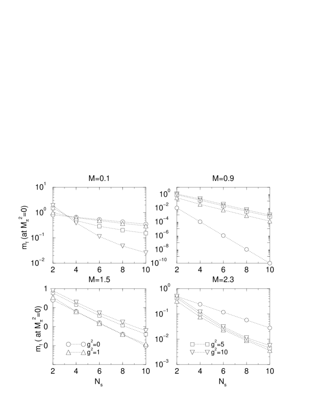
FIG. 11.: $m_{f}(M_{\pi}=0)$ as a function of $N_{s}$ for fixed $M,g^{2}$.

  

FIG. 12.: $N_{s}$ dependence of the phase boundary for $M=-0.1,0.9$. The horizontal axis represents $m_{f}$ while the vertical axis is $g^{2}$.

FIG. 13.: $\widetilde{M}_{\pi}^{2}$ and $\langle\bar{q}q\rangle=m_{f}-\sigma$ as a function of $m_{f}$. $N_{s}=4,g^{2}=1.0$.

FIG. 14.: $\langle\bar{q}q\rangle=m_{f}-\sigma$ as a function of $M$. $N_{s}=20,g^{2}=1.0$.

  

FIG. 15.: $\widetilde{M}_{\pi}^{2}f_{M}^{2}$ as a function of $M$. $g^{2}=1.0$ and $g^{2}=5.0$ for $N_{s}=2,4,6,8,12$.

FIG. 16.: $\sigma/\Lambda$ and $\widetilde{M}_{\pi}^{2}$ as a function of $a\Lambda$ for fixed $M$. The continuum limit is taken using the (Wilson like) scaling relations in (73-75).

FIG. 17.: $\sigma/\Lambda$ and $\widetilde{M}_{\pi}^{2}$ as a function of $a\Lambda$ at $Ns=20$.

FIG. 18.: $\sigma/\Lambda$ and $\widetilde{M}_{\pi}^{2}$ as a function of $a\Lambda$ at $M=0.9$. The DWF scaling relations in (90-92) are employed.

FIG. 19.: $N_{s}$ dependence of $\widetilde{M}_{\pi}^{2}$ as a function of $m_{f}$.

REFERENCES

- [1] H. B. Nielsen and M. Ninomiya, Nucl. Phys. B185, 20 (1981); erratum: ibid. B195, 541 (1982); Nucl. Phys. B193, 173 (1981); Phys. Lett. B105, 219 (1981).
- [2] L. H. Karsten, Phys. Lett. B104, 315 (1981).
- [3] K. Wilson; in New Phenomena in Subnuclear Physics, ed. Zichichi (Erice, 1975) (Plenum, New York, 1977).
- [4] L. Karsten and J. Smit, Nucl. Phys. B 183, 103 (1981).
- [5] D. B. Kaplan, Phys. Lett. B 288, 342 (1992); Nucl. Phys. B(Proc. Suppl.) 30, 597 (1993).
- [6] Y. Shamir, Nucl. Phys. B 406, 90 (1993).
- [7] Furman and Shamir, Nucl. Phys. B 439, 54 (1995).
- [8] S. Aoki and Y. Taniguchi, Phys. Rev. D58, 074505 (1998); Nucl. Phys. B (Proc. Suppl.) 63, 20 (1998).
-
[9]
T. Blum and A. Soni,
Phys. Rev. D56, 174 (1997);
Phys. rev. Lett. 79, 3595 (1997).
T. Blum, “Domain wall fermions in vector gauge theories”, hep-lat/9810017. -
[10]
P. Chen et al (Columbia lattice group),
“Toward the Chiral Limit of QCD:
Quenched and Dynamical Domain Wall Fermions”,
hep-lat/9812011.
P.Vranas and Columbia lattice group, “Dynamical lattice QCD thermodynamics and the symmetry with domain wall fermions”, hep-lat/9903024. - [11] S. Aoki, Phys. Rev. D30, 2653 (1984) .
- [12] S. Aoki, A. Ukawa and T. Umemura, Phys. Rev. Lett. 76, 873 (1996) .
- [13] S. Aoki, T. Kaneda and A. Ukawa, Phys. Rev. D56, 1808, (1997) .
- [14] Sinya Aoki and Kiyoshi Higashijima, Prog. of Theor. Phys. 76, 521 (1986) .
- [15] P. Vranas, I. Tziligakis and J. Kogut, “Fermion-scalar interactions with domain wall fermions”, hep-lat/9905018 .
- [16] Ikuo Ichinose and Keiichi Nagao, “Pion Mass and the PCAC Relation in the Overlap Fermion Formalism: Gauged Gross-Neveu Model on a Lattice”, hep-lat/9905001 .
- [17] T. Izubuchi, J. Noaki and A. Ukawa, Phys. Rev. D58, 114507 (1998).
- [18] P. Vranas, Phys. Rev. D57, 1415 (1998); Nucl. Phys. B (Proc. Suppl.) 63, 605 (1998).
- [19] H. Neuberger, Phys. Rev. D57, 5417 (1998).
- [20] Yoshio Kikukawa and Atsushi Yamada, Phys. Lett. B448, 265 (1999).
- [21] Stephan Sharpe and Robert Singleton, Jr., Phys. Rev. D58, 74501 (1998).