MAGNETIC FIELD ON LATTICE U(1)-HIGGS AND SU(2)$\times$U(1)-HIGGS THEORIES

Abstract

External (hyper)magnetic field can modify the phase structure in U(1) gauge+Higgs (Landau-Ginzburg) and SU(2)$\times$U(1) gauge+Higgs (Standard Model) theories. In this talk I discuss how the magnetic field can be implemented on the lattice, and summarize the effects on symmetry breaking phase transitions.

1 Introduction

Theories with a U(1) gauge field allow gauge invariant (global) magnetic fields. In this talk I discuss the Higgs field driven phase transitions in 3-dimensional U(1) gauge+Higgs[1] and SU(2)$\times$U(1) gauge+Higgs[2] theories, and especially what happens to the transitions when an external magnetic field is applied. As is appropriate for the topic of this workshop, I shall point out some similar features to lattice QCD simulations with a fixed baryon number.

Several reasons make U(1) gauge+Higgs theory with external magnetic field interesting: first of all, it is the dimensionally reduced version of 3+1-dim. scalar QED at high temperatures.[1] It also is equivalent to the Ginzburg-Landau theory of superconductivity, and it is very useful as a “toy model” for studying the behaviour of string-like defects in cosmology (Nielsen-Olesen strings). On the other hand, 3d SU(2)$\times$U(1) gauge+Higgs theory is precisely the high-temperature effective theory of the Standard Model (and of many of its extensions). The physical consequences of the electroweak phase transition in the early Universe can be substantially modified in the presence of a hypermagnetic field (homogeneous in microscopic scales).

2 U(1)+Higgs Theory with Magnetic Field

The action of the U(1)+Higgs theory in the continuum is

$$S=\int d^{3}x\big{[}\mbox{${\frac{1}{4}}$}F_{ij}F_{ij}+(D_{i}\phi)^{*}D_{i}\phi+m_{3}^{2}|\phi|^{2}+\lambda_{3}|\phi|^{4}\big{]}\,,$$ (1)

where the couplings $e_{3}^{2}$, $m^{2}_{3}$ and $\lambda_{3}$ are dimensionful. The lattice action (with non-compact U(1)) can be written as

$$S_{L}=\sum_{x}\bigg{[}\beta_{G}\sum_{ij}{\frac{1}{2}}\alpha_{ij}^{2}-\beta_{H}\sum_{i}\mbox{Re\,}(\phi^{*}_{x}U_{x,i}\phi_{x+i})+\beta_{2}|\phi|^{2}+\beta_{4}|\phi|^{4}\bigg{]}\,,$$ (2)

where the plaquette $\alpha_{x,ij}=\alpha_{x,i}+\alpha_{x+i,j}-\alpha_{x+j,i}-\alpha_{x,j}$ and $U_{x,i}=\exp i\alpha_{x,i}$. The gauge coupling is $\beta_{G}=1/(e_{3}^{2}a)$, and the relations of $\beta_{H}$, $\beta_{2}$ and $\beta_{4}$ to the continuum parameters are given in[1]. Note that the 3d theory is superrenormalizable, and it has a well-defined continuum limit.

How should one proceed in order to introduce an external magnetic field in the system? For definiteness, let us fix ${\bf H}\parallel{\bf B}\parallel\hat{e}_{3}$. The customary way of introducing the field is to add a source term to the action:

$$Z(H)=\int[dUd\phi]\exp\big{[}\mbox{$-S+\int dxB(x)H$}\big{]}\,.$$ (3)

Here $B(x)=F_{12}(x)=\beta_{G}^{2}{e_{3}^{3}}\alpha_{12}(x)$ is the (local) magnetic field. However, this approach does not work on a finite lattice with periodic boundary conditions: if we consider any plane with a fixed $x_{3}$-coordinate, then $\sum_{x_{1},x_{2}}\alpha_{12}(x)=\sum_{\partial A}{\bf\alpha}\cdot\hat{e}_{\partial A}=0$, where $\partial A$ is the boundary of the (1,2)-plane. Thus, external field $H$ has no effect on $Z$!

One method to solve this problem is to use modified boundary conditions.[1, 2] For example, let us choose link $\alpha_{1}(1,1,x_{3})$ on each (1,2)-plane, and use a non-periodic boundary condition for this link alone:

$$\alpha_{1}(1,1,x_{3})=\alpha_{1}(1,N,x_{3})+\Delta\,,\mbox{~{}~{}~{}otherwise $\alpha_{i}$ periodic.}$$ (4)

Here $L^{3}=(aN)^{3}$ is the size of the lattice. If, for the time being, we neglect the Higgs field, this extra ‘twist’ can distribute itself evenly on all (1,2)-plaquettes: $\langle\alpha_{12}\rangle=\Delta/N^{2}$, corresponding to a homogeneous magnetic field $B_{3}=\Delta/(e_{3}L^{2})$. It should be noted that the particular choice of the link in Eq. (4) does not give that link a special status: the action — and physics — remains translationally invariant. If we now make $\Delta$ a dynamical variable, the source term in Eq. (3) simply becomes $\Delta H/e_{3}$, and canonical simulations become possible.

However, when the Higgs field is taken into account, a new condition arises: the hopping term in Eq. (2) is translation invariant only if the condition $\Delta=2\pi n$, $n$ integer, is satisfied. If this is not the case, there will be a localized ‘defect’ on the link $\alpha_{1}(1,1,z)$, and these configurations are unphysical. In principle, one may still attempt to update $n$ dynamically in integer units, but these updates are extremely strongly suppressed. In practice the total flux $\Phi_{B}$ remains fixed, and we have an ensemble

$$Z(\Phi_{B})=\int[dUd\phi]e^{-S}\delta(\Phi_{B}(U)-\Phi_{B})\,,\hskip 11.38109pt\Phi_{B}=2\pi n/e_{3}\,.$$ (5)

In what follows I call this a microcanonical ensemble. When one scans the phase space of the system, this ensemble causes several problems. For example, let us now consider the case $\lambda_{3}/e_{3}^{2}\ll 1$, which (in terms of Ginzburg-Landau theory) describes a type I superconductor. When $m_{3}^{2}$ (which is now a function of temperature $T$) is decreased from positive values to negative ones, the system has a strong 1st order phase transition from the symmetric to the broken (Higgs) phase. In the canonical constant $H$ ensemble Eq. (3), the magnetic field cannot penetrate the broken phase, forcing $B=0$ due to Meissner effect, as shown schematically in Fig. 1. However, in the microcanonical ensemble (5) the flux is fixed and cannot vanish. The system can accommodate this only by forming a mixed phase: the magnetic field penetrates the volume through a cylinder with a small cross-sectional area, so that the field strength inside the cylinder is large enough to support unbroken phase at this temperature.

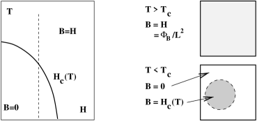
Figure 1: Left: the phase diagram of type I superconductor in $H,T\sim m_{3}^{2}$ plane. Right: (1,2)-plane cross sections of the system in the microcanonical ensemble Eq. (5). System goes in a mixed phase when $T<T_{c}$, where $H_{c}(T_{c})=\Phi_{B}L^{2}$. In the mixed phase the flux is concentrated in a subvolume with a cross-sectional area $A$ so that $AB=AH_{c}(T)=\Phi_{B}$.

An immediate consequence of the existence of the mixed phase is the ‘rounding off’ of the phase transition: if we are in the mixed phase and increase $T$, the symmetric phase domain grows smoothly, until at $T=T_{c}$ it takes over the whole volume. There are no discontinuities in thermodynamical densities when the external parameters ($\Delta$, couplings) are varied. This is in strong contrast to the canonical ensemble, which typically displays strong discontinuities in 1st order phase transitions. This property is a generic feature of almost any ‘microcanonical-like’ ensembles. For example, a very analogous situation occurs in QCD simulations with a fixed baryon number,[5] where the transition from hadronic phase to quark-gluon plasma becomes continuous.

One way to work around the quantization condition in Eq. (5) is to use multicanonical  (or related) methods to interpolate $\Delta=2\pi n$ from $n$ to $n+1$, for example. Even when the non-integer values of $n$ do not correspond to physical configurations, the free energy difference obtained from the integral

$$\delta F(n\rightarrow n+1)=\int_{2\pi n}^{2\pi(n+1)}d\Delta\,{\frac{\partial F}{\partial\Delta}}$$ (6)

is a fully physical quantity. In type II domain $\lambda_{3}/e_{3}^{2}>1$, where the magnetic field in the Higgs phase forms unit flux vortices, the integration method was succesfully used to measure the vortex tension = free energy/length.[1] This, in turn, can be used as an order parameter between the symmetric/broken phases.

3 SU(2)$\times$U(1)-Higgs Theory

3d SU(2)$\times$U(1) gauge+Higgs theory is an effective theory of high $T$ Standard Model.[2, 3] The Lagrangian of the theory is

$$\mbox{${\frac{1}{4}}$}F^{a}_{ij}F^{a}_{ij}+\mbox{${\frac{1}{4}}$}B_{ij}B_{ij}+(D_{i}\phi)^{\dagger}D_{i}\phi+m_{3}^{2}\phi^{\dagger}\phi+\lambda_{3}(\phi^{\dagger}\phi)^{2}\,,$$ (7)

where $F_{ij}^{a}$ and $B_{ij}$ are SU(2) and U(1) field strength tensors with gauge fields $A_{i}^{a}$ and $B_{i}$, the covariant derivative $D_{i}=\partial_{i}+ig_{3}A_{i}+ig^{\prime}_{3}B_{i}/2$, and the Higgs field $\phi$ is a complex doublet. Here the 3d gauge couplings $g_{3}^{2}\approx g^{2}T$, $g^{\prime}_{3}{}^{2}\approx g^{\prime}{}^{2}T$, and we fix $z=g^{\prime}{}^{2}_{3}/g^{2}_{3}=0.3$. The results are conveniently expressed in terms of dimensionless variables $x=\lambda_{3}/g_{3}^{2}$ and $y=m_{3}^{2}/g_{3}^{4}$.

Since Eq. (7) contains the hypercharge U(1) field, we can study the phase transition in the presence of an external hypermagnetic field with similar methods as for the U(1)-Higgs theory above. As before, the flux is quantized, and we are restricted to the microcanonical ensemble as in Eq. (5). However, in the present case the hypermagnetic field can penetrate the broken (Higgs) phase as an ordinary magnetic field, albeit with a cost in free energy. Again, at small $x$ the transition is of 1st order, and in the microcanonical ensemble we expect the single transition line to be split into a band of mixed phase. Using tree-level analysis, this is shown in Fig. 2. At large $x$ there is a region where neither symmetric nor broken Higgs phases are stable (again, at tree level!), and it is possible that one finds here a new vortex-like Ambjørn-Olesen[6] phase, which breaks translational invariance.

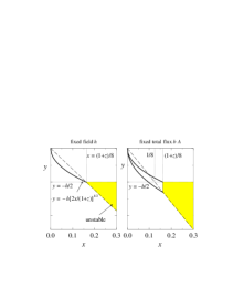
Figure 2: The tree-level phase diagram in SU(2)$\times$U(1) gauge+Higgs theory with fixed external field $H$ (canonical ensemble, left) and fixed total flux $B\times$ area (microcanonical ensemble, right). The single first order transition line at small $x$ splits into a band where a symmetric/broken mixed phase can be found. The shaded region at large $x$ shows where the Ambjørn-Olesen phase can be expected to appear.[6]

Figure 3: The measured mixed phase band when the flux density is $B_{Y}\approx 8g^{4}T^{2}/3g^{\prime}$.

Indeed, in extensive lattice simulations we do observe a mixed phase, as shown in Figs. 3 and 4. Not surprisingly, though, the quantitative differences from tree-level results are large. On the other hand, at larger $x$ we do not observe the Ambjørn-Olesen phase. Instead the broken and symmetric phases appear to be smoothly connected in this region, compatible with the observed behaviour in the absence of magnetic field. For all of the details, see refs.[2, 7].

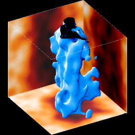
Figure 4: A mixed phase configuration in SU(2)$\times$U(1)+Higgs theory. The hypermagnetic flux preferentially goes through a cylinder of the symmetric phase embedded in the bulk broken phase.

References

References

- [1] K. Kajantie et al, Nucl. Phys. B 546, 351 (1999) [hep-ph/9809334]; Nucl. Phys. B 520, 345 (1998) [hep-lat/9711048]; Phys. Lett. B 423, 137 (1998) [hep-ph/9710538]; in preparation.
- [2] K. Kajantie et al, Nucl. Phys. B 544, 357 (1999) [hep-lat/9809004]; Nucl. Phys. B 493, 413 (1997) [hep-lat/9612006].
- [3] K. Farakos et al, Nucl. Phys. B 425, 67 (1994) [hep-ph/9404201]; K. Kajantie et al, Nucl. Phys. B 458, 90 (1996) [hep-ph/9508379].
- [4] P.H. Damgaard, U.M. Heller, Phys. Rev. Lett. 60, 1246 (1988); Nucl. Phys. B 309, 625 (1988).
- [5] O. Kaczmarek, these proceedings; J. Engels et al, BI-TP-99-04, [hep-lat/9903030].
- [6] J. Ambjørn and P. Olesen, Nucl. Phys. B 315, 606 (1989); Nucl. Phys. B 330, 193 (1990); Int. J. Mod. Phys. A 5, 4525 (1990).
- [7] K. Kajantie et al, in preparation.