Abstract

The fermion determinant and the chiral anomaly of lattice Dirac operator $D$ on a finite lattice are investigated. The condition for $D$ to reproduce correct chiral anomaly at each site of a finite lattice for smooth background gauge fields is that $D$ possesses exact zero modes satisfying the Atiyah-Singer index theorem. This is also the necessary condition for $D$ to have correct fermion determinant ( ratio ) which plays the important role of incorporating dynamical fermions in the functional integral. We outline a scheme for dynamical fermion simulation of lattice QCD with topologically proper $D$.

PACS numbers: 11.15.Ha, 11.30.Fs, 11.30.Rd

1 Introduction

The fermion determinant, $\mbox{det}(D)$, of a Dirac operator $D$, is proportional to the exponentiation of the one-loop effective action which is the summation of any number of external sources interacting with one internal fermion loop. It is one of the most crucial quantities to be examined in any lattice fermion formulations. In numerical simulations of lattice QCD, its ratio between two successive gauge configurations determines whether the effects of dynamical quarks are properly incorporated, which are believed to be cruical to bring the ab initio predictions of lattice QCD to agree with the experimental data. Another important quantity in QCD is the chiral anomaly which breaks the global chiral symmetry of massless QCD through the internal quark loop. In the case of the axial current coupling to two external photons, the axial anomaly [1] provides a proper account of the decay rate of $\pi^{0}\to\gamma\gamma$. For the flavor singlet axial current coupling to two gluons, the presence of chiral anomaly but no associated Goldstone boson posed the $U_{A}(1)$ problem which was resolved by ’t Hooft [2], after taking into account of the topologically nontrivial gauge configurations, the instantons. This may also provide an explanation why the $\eta$ ( $\eta^{\prime}$ ) particle is much heavier than the $\pi$’s ( $K$’s ). Lattice QCD should be designed to provide nonperturbative and quantitive answers to all these and related problems. However, these goals could not be attained if the lattice Dirac fermion operator does not reproduce correct chiral anomaly or the fermion determinant ( ratio ) on a finite lattice without fine-tuning any parameters. Furthermore, lattice QCD should realize the spontaneous breaking of chiral symmetry in massless QCD, which gives massless Goldstone bosons and thus leads to a correct and detailed description of the properties of the strong interactions at low energy [3].

A basic requirement for lattice Dirac operator $D$ is that, on a finite lattice with any prescribed smooth background gauge field which has a well-defined topological charge, $D$ possesses exact zero modes satisfying the Atiyah-Singer index theorem ( i.e., $D$ is topologically proper ) without fine tuning any parameters. Here we would like to emphasize the importance of having exact zero modes on a finite lattice without fine tuning any parameters. If the zero modes can only be obtained by fine tuning parameters, then it is impossible to tune the parameters for every gauge configuration generated during a Monte Carlo simulation.

For any $D$ satisfying this requirement, the sum of the anomaly function over all sites must be correct, and is equal to two times of the topological charge of the background gauge field. If it turns out that the anomaly function of $D$ at some of the sites do not agree with the Chern-Pontryagin density, we can perform the following topologically invariant transformation

$${\cal T}(R):\hskip 11.38109ptD^{\prime}={\cal T}(R)[D]\equiv D(\mbox{1I}+RD)^{-1}$$ (1)

with some operator $R$ such that $D^{\prime}$ is local, then the anomaly function of $D^{\prime}$ would be in good agreement with the Chern-Pontryagin density at each site. It suffices to choose $R$ to be a hermitian operator which is local in the position space and trivial in the Dirac space. The terminology, topologically invariant, refers to the property that the zero modes and the index of $D$ are invariant under the transformation (1). Note that it is not necessary to perform any fine tunings of $R$ since any local $D^{\prime}$ would give the correct chiral anomaly. Evidently, the set of transformations, $\{{\cal T}(R)\}$, with the group multiplication defined by

$$({\cal T}(R_{1})\circ{\cal T}(R_{2}))[D]={\cal T}(R_{1})[{\cal T}(R_{2})[D]],$$ (2)

form an abelian group with the group parameter space $\{R\}$, due to the following basic property,

$${\cal T}(R_{1})\circ{\cal T}(R_{2})={\cal T}(R_{1}+R_{2}).$$ (3)

In the topologically trivial sector, $D^{-1}$ exists and (1) becomes

$$D^{\prime-1}=D^{-1}+R.$$ (4)

Then there exists a unique

$$R_{c}=-{1\over 2}\{D^{-1},\gamma_{5}\}\gamma_{5}$$ (5)

such that

$$D_{c}^{-1}=D^{-1}+R_{c}$$ (6)

is chirally symmetric, i.e.,

$$\gamma_{5}D_{c}^{-1}+D_{c}^{-1}\gamma_{5}=0.$$ (7)

From the physical point of view, we must require the existence of a chirally symmetric $D_{c}={\cal T}(R_{c})[D]$ such that in the free fermion limit $D_{c}(p)\to i\gamma_{\mu}p_{\mu}$ as $p\to 0$, otherwise, $D$ is irrelevant to massless QCD. In general, we assume that there exists

$$D_{c}=D(\mbox{1I}+R_{c}D)^{-1}$$ (8)

such that

$$D_{c}\gamma_{5}+\gamma_{5}D_{c}=0.$$ (9)

If $D(D_{c})$ is topologically proper, then $D(D_{c})$ must be free of species doubling, thus $D_{c}$ is non-local, according to the Nielson-Ninomiya no-go theorem [6]. Furthermore, $D_{c}$ has singularities in topologically nontrivial background gauge fields [7]. Substituting (8) into (9), we obtain

$$D\gamma_{5}+\gamma_{5}D=-2DR_{c}\gamma_{5}D.$$ (10)

This is the rejuvenated Ginsparg-Wilson relation [8]. In general, for any lattice Dirac operator $D$, if the chirally symmetric $D_{c}={\cal T}(R_{c})[D]$ exists, then $D$ must satisfy the Ginsparg-Wilson relation. From this viewpoint, the Ginsparg-Wilson relation really does not specify the important attribute of a Dirac operator, namely its topological characteristics [7]. Only for $D$ is topologically proper ( e.g., the overlap-Dirac operator [9] ), $D$ ( or its transform $D^{\prime}=D(\mbox{1I}+RD)^{-1}$ ) can be used for lattice QCD, then the attractive features pointed out in refs. [10, 11] can be realized on a finite lattice. If $D$ is topologically proper but nonlocal, the transformation (1) can be used to obtain a local $D^{\prime}$ such that the anomaly function at each site of a finite lattice could agree with the corresponding Chern-Pontryagin density for smooth background gauge fields. Moreover, the locality of $D^{\prime}$ also implies that its fermion determinant ratio ( with the zero modes omitted ) would agree with the corresponding value in continuum.

2 The Anomaly Function

In general, we consider lattice Dirac operator $D$ which breaks the continuum chiral symmetry according to

$$D\gamma_{5}+\gamma_{5}D=B$$ (11)

where $B$ is a generic operator which is usually taken to be irrelevant ( i.e., vanish in the limit $a\to 0$ ). However, we can construct the chirally symmetric action

$${\cal A}_{s}=\bar{\psi}D_{s}\psi$$ (12)

using the chirally symmetric part of $D$,

$$D_{s}={1\over 2}(D-\gamma^{5}D\gamma^{5}).$$ (13)

Here the Dirac, flavor and internal symmetry indices are all suppressed. Then ${\cal A}_{s}$ has the usual chiral symmetry, and the divergence of the associated Noether current is

$$\partial^{\mu}J^{5}_{\mu}(x)=\bar{\psi}_{x}\gamma^{5}(D\psi)_{x}+(\bar{\psi}D)_{x}\gamma^{5}\psi_{x}-{1\over 2}(\bar{\psi}B)_{x}\psi_{x}-{1\over 2}\bar{\psi}_{x}(B\psi)_{x}$$ (14)

which satisfies the conservation law,

$$\sum_{x}\partial^{\mu}J^{5}_{\mu}(x)=0.$$ (15)

As usual, the lattice is taken to be finite with periodic boundary conditions, and $\partial_{\mu}J_{\mu}^{5}(x)$ is defined by the backward difference of the axial current

$$\partial_{\mu}J_{\mu}^{5}(x)=\sum_{\mu}\ [J_{\mu}^{5}(x)-J_{\mu}^{5}(x-\hat{\mu})\ ]$$ (16)

such that it is parity even under the parity transformation, and the conservation law Eq. (15) is also satisfied.

If $D$ does not possess exact zero modes in the background gauge field , then the fermionic average of $\partial^{\mu}J^{5}_{\mu}(x)$ can be evaluated as

$$\left<\partial^{\mu}J^{5}_{\mu}(x)\right> = {1\over Z}\int[d\psi][d\bar{\psi}]\partial^{\mu}J^{5}_{\mu}(x)\exp(-\bar{\psi}D\psi)$$ (17)

$$Z = \int[d\psi][d\bar{\psi}]\exp(-\bar{\psi}D\psi)$$ (18)

Using (14), we obtain

$$\left<\partial^{\mu}J^{5}_{\mu}(x)\right>={1\over 2}\ \mbox{tr}\left[(BD^{-1})(x,x)+(D^{-1}B)(x,x)\right]\equiv{\cal A}_{n}(x)$$ (19)

where the trace runs over the Dirac, flavor and internal symmetry indices. The RHS of Eq. (19) is identified to be the anomaly function of $D$. If the chirally symmetric limit of (1), i.e., $D_{c}={\cal T}(R_{c})[D]$ exists, then $D$ satisfies the Ginsparg-Wilson relation (10) and the anomaly function becomes

$${\cal A}_{n}(x)=-\mbox{tr}\left[\gamma_{5}(R_{c}D)(x,x)+\gamma_{5}(DR_{c})(x,x)\right]$$ (20)

However, for any $D$ which does not possess exact zero modes in the background gauge field, the sum of the anomaly function (19) over all sites must vanish due to the conservation law, Eq. (15),

$$\sum_{x}{\cal A}_{n}(x)=0\ .$$ (21)

This implies that if ${\cal A}_{n}(x)$ is not zero identically for all $x$, then it must fluctuate from positive to negative values with respect to $x$. The latter case is exactly what happens to the anomaly function of the standard Wilson-Dirac fermion operator.

On the other hand, if $D$ possesses exact zero modes in topologically nontrivial background gauge fields, then $D^{-1}$ is not well defined. In this case, one needs to introduce an infinitesimal mass $m$ and evaluate (17) with $D$ replaced by $\hat{D}=D+mf[D]$ ( where $f[D]$ is any functional of $D$, which has eigenvalue one for the exact zero modes of $D$ ), and finally take the limit ( $m\to 0$ ), i.e.,

$$\left<\partial^{\mu}J^{5}_{\mu}(x)\right> = \lim_{m\to 0}{1\over Z}\int[d\psi][d\bar{\psi}]\partial^{\mu}J^{5}_{\mu}(x)\exp(-\bar{\psi}\hat{D}\psi)$$ (22)

$$Z = \int[d\psi][d\bar{\psi}]\exp(-\bar{\psi}\hat{D}\psi)$$ (23)

Inserting (14) into (22), we obtain

$$\left<\partial^{\mu}J^{5}_{\mu}(x)\right> = \lim_{m\to 0}{1\over 2}\ \mbox{tr}\left[(B\hat{D}^{-1})(x,x)+(\hat{D}^{-1}B)(x,x)\right]$$ (24)

$$+2\sum_{s=1}^{N_{+}}[\phi_{s}^{+}(x)]^{\dagger}\phi_{s}^{+}(x)-2\sum_{t=1}^{N_{-}}[\phi_{t}^{-}(x)]^{\dagger}\phi_{t}^{-}(x)$$

where $\phi_{s}^{+}$ and $\phi_{t}^{-}$ are normalized eigenfunctions of $D$ with eigenvalues $\lambda_{s}=\lambda_{t}=0$ and chiralities $+1$ and $-1$ respectively. The first term on the RHS of Eq. (24) is identified to be the anomaly function of $D$,

$${\cal A}_{n}(x)=\lim_{m\to 0}{1\over 2}\ \mbox{tr}\left[(B\hat{D}^{-1})(x,x)+(\hat{D}^{-1}B)(x,x)\right]$$ (25)

Then summing Eq. (24) over all sites and using Eq. (15), we obtain

$$N_{-}-N_{+}={1\over 2}\sum_{x}{\cal A}_{n}(x)$$ (26)

This is the index theorem for any lattice Dirac operator on a finite lattice, in any background gauge field. In the case $D$ does not possess any exact zero modes, Eq. (26) reduces to Eq. (21). Equation (26) implies that the sum of the anomaly function over all sites must be a well defined even integer for any background gauge field, however, it does not necessarily imply the Atiyah-Singer index theorem for smooth background gauge fields. This can be seen as follows. Since $D$ does not have exact zero modes in a trivial gauge background, the index of $D$ must be proportional to the topological charge $Q$ of the smooth background gauge field. Now, if $Q$ is an integer, then the proportional constant must be an integer, otherwise their product in general cannot be an integer. Denoting this integer multiplier by $c[D]$, we have

$$N_{-}-N_{+}=c[D]\ Q\ n_{f}$$ (27)

where $n_{f}$ is number of fermion flavors. In particular, for $n_{f}=Q=1$, $c[D]=N_{-}-N_{+}$. Here we have assumed that $c[D]$ is constant for smooth background gauge fields. This is a reasonable assumption since $c[D]$ is an intrinsic characteristics of $D$. However, when the gauge field becomes rough, we expect that Eq. (27) would break down. If one insists that Eq. (27) holds even for rough gauge configurations, then $c[D]$ cannot be an integer constant due to the highly nonlinear effects of the gauge field. It is easy to deduce that, in general, $c[D]$ is a rational number functional of $D$, which in turn depends on the gauge configuration, but it becomes an integer constant only for smooth gauge configurations. The topological characteristics of $D$, $c[D]$, was first discussed in ref. [7], and was investigated in ref. [12] for the Neuberger-Dirac operator. Equation (27) constitutes the index theorem for any lattice Dirac operator on a finite lattice, in any background gauge field with integer topological charge. We can classify $D$ according to its response in a smooth nontrivial background gauge field. If $D$ does not possess any zero modes, then $c[D]=0$, $D$ is called topologically trivial. If $c[D]=1$, (27) becomes Atiyah-Singer index theorem, then $D$ is called topologically proper. If $c[D]$ is not equal to zero or one, then $D$ is called topologically improper.

Now we try to obtain a general expression for the anomaly function satisfying (26) and (27). Consider the gauge configuration with constant field tensors, e.g., $F^{a}_{12}(x)={2\pi q_{1}\over L_{1}L_{2}}$, $F^{a}_{34}(x)={2\pi q_{2}\over L_{3}L_{4}}$ and other $F$’s are zero, where $q_{1}$ and $q_{2}$ are integers. Then the topological charge of this configuration is

$$Q={1\over 32\pi^{2}}\ \sum_{x}\epsilon_{\mu\nu\lambda\sigma}\ F_{\mu\nu}^{a}(x)F_{\lambda\sigma}^{b}(x+\hat{\mu}+\hat{\nu})\ \mbox{tr}\{t_{a}t_{b}\}=n\ q_{1}\ q_{2}$$ (28)

which is an integer. Here $t_{a}$ and $t_{b}$ are generators of the internal symmetry group with the normalization $\mbox{tr}\{t_{a}t_{b}\}=n\ \delta_{ab}$. If $D$ is local, then it is reasonable to assume that ${\cal A}_{n}(x)$ is constant for all $x$. From Eqs. (26)-(28), we obtain

$${\cal A}_{n}(x)={n_{f}\over 16\pi^{2}}\ c[D]\ \epsilon_{\mu\nu\lambda\sigma}\ F_{\mu\nu}^{a}(x)F_{\lambda\sigma}^{b}(x+\hat{\mu}+\hat{\nu})\ \mbox{tr}\{t^{a}t^{b}\}\ .$$ (29)

However, this implies that any local $D$ would yield the correct anomaly function on a finite lattice, up to the integer factor $c[D]$. In reality, this cannot be true in general. The crux of the problem is due to the fact that when $D$ is topological trivial, i.e. $c[D]=0$ in the index theorem (27), the anomaly function ${\cal A}_{n}(x)$ does not necessarily vanish identically at each site, but it can fluctuate from positive to negative values provided that its sum over all sites is zero. This is the complementary solution to the homogeneous equation $\sum_{x}{\cal A}_{n}(x)=0$. Using Eq. (19), we can write the general form of the complementary solution as

$${\cal A}^{(h)}(x)=\sum_{\mu}\ [G_{\mu}(x)-G_{\mu}(x-\hat{\mu})]\equiv\partial_{\mu}G_{\mu}(x)$$ (30)

where $G_{\mu}(x)$ is any local and gauge invariant function. Then the general solution of the anomaly function is the sum of the complementary solution (30) and the particular solution (29),

$${\cal A}_{n}(x) = {n_{f}\over 16\pi^{2}}\ c[D]\ \epsilon_{\mu\nu\lambda\sigma}\ F_{\mu\nu}^{a}(x)F_{\lambda\sigma}^{b}(x+\hat{\mu}+\hat{\nu})\ \mbox{tr}\{t^{a}t^{b}\}$$ (31)

$$+\sum_{\mu}\ [G_{\mu}(x)-G_{\mu}(x-\hat{\mu})]$$

In general, $G_{\mu}(x)$ depends on the background gauge field as well as the lattice Dirac operator $D$. If ${\cal A}^{(h)}(x)$ does not vanish in the presence of a constant gauge background, then ${\cal A}_{n}(x)$ must be different from the continuum chiral anomaly, hence this $D$ should be abandoned. Only when ${\cal A}^{(h)}(x)$ vanishes identically for any smooth gauge background, $D$ can reproduce the correct chiral anomaly for $c[D]=1$ ( e.g., the Neuberger-Dirac operator ). On the other hand, the pathologies of the standard Wilson-Dirac operator are : $c[D]=0$ and ${\cal A}^{(h)}(x)\neq 0$.

Now we consider $D$ with anomaly function ${\cal A}_{n}(x)$ satisfying (29) in a constant gauge background. Then we introduce local fluctuations [ e.g., the sinusoidal terms in Eqs. (63)-(66) ] to the background gauge field and/or increase its topological charge $Q$. Then $c[D]$ in Eqs. (29) and (27) may remain constant provided that the local fluctuations of the gauge fields are not too violent and/or $Q$ is not too large. When the gauge background becomes so rough that $D$ is non-local, then Eq. (29) is no longer valid, but the index theorem, Eq. (27) may still hold with the same $c[D]$. In this case, the anomaly function ${\cal A}_{n}(x)$ can be expressed in terms of the general formula (31) with the same $c[D]$ but nonvanishing $\partial_{\mu}G_{\mu}(x)$. If we keep on increasing the roughness of the gauge background, then $D$ will undergo a topological phase transition, and $c[D]$ in Eqs. (27) and (31) will become another integer or even a fraction ( Explicit examples of topological phase transition will be demonstrated in Section 4 ). In general, Eq. (31) constitutes the anomaly function for any lattice Dirac operator $D$ on a finite lattice, in any background gauge field. However, only when ${\cal A}^{(h)}(x)=0$ and $c[D]=1$, the anomaly function can agree with the Chern-Pontryagin density.

If the chirally symmetric limit of $D$, i.e., $D_{c}={\cal T}(R_{c})[D]$, exists, then $D$ satisfies the Ginsparg-Wilson relation (10), and its anomaly function (25) becomes exactly in the same form of Eq. (20). Substituting Eq. (20) into the LHS of Eq. (31), we obtain

$${\cal A}_{n}(x) = -\mbox{tr}\left[\gamma_{5}(R_{c}D)(x,x)+\gamma_{5}(DR_{c})(x,x)\right]$$ (33)

$$= {n_{f}\over 16\pi^{2}}\ c[D]\ \epsilon_{\mu\nu\lambda\sigma}\ F_{\mu\nu}^{a}(x)F_{\lambda\sigma}^{b}(x+\hat{\mu}+\hat{\nu})\ \mbox{tr}\{t^{a}t^{b}\}$$

$$+\sum_{\mu}\ [G_{\mu}(x)-G_{\mu}(x-\hat{\mu})]$$

which agrees with the results obtained in ref. [7, 13]. For $U(1)$ lattice gauge theory with ”admissible” background gauge configurations, Eq. (33) agrees with the result derived by Lüscher [14]. For the Overlap-Dirac operator, in the weak coupling limit or the classical continuum limit, we have $\partial_{\mu}G_{\mu}(x)=0$, then Eq. (33) agrees with the results derived by Kikukawa and Yamada [15], Fujikawa [16], Adams [17] and Suzuki [18] respectively.

Inserting Eq. (25) [ Eq. (20) ] into Eq. (26), we obtain

$$N_{-}-N_{+}=-{1\over 2}\sum_{x}\mbox{tr}\left[\gamma_{5}(R_{c}D)(x,x)+\gamma_{5}(DR_{c})(x,x)\right]\$$ (34)

which agrees with the index theorem for Ginsparg-Wilson fermion [19, 20]. Note that (34) does not necessarily imply the Atiyah-Singer index theorem for smooth background gauge fields with integer topological charge.

If the lattice Dirac operator $D$ does not have exact zero modes in the presence of topologically non-trivial background gauge fields, however, it manages to possess exact zero modes in a certain limit, say, for example, the Wilson-Dirac fermion operator [5] in the classical continuum limit ( i.e., zero lattice spacing with infinite number of sites in each direction ). Then on any finite lattice, this lattice Dirac operator cannot reproduce the correct anomaly function for topologically non-trivial background gauge fields, since the sum of the anomaly function (19) over the entire lattice must be zero due to the conservation law (15),

$${1\over 2}\sum_{x}\ \mbox{tr}\left[(BD^{-1})(x,x)+(D^{-1}B)(x,x)\right]=\sum_{x}\left<\partial^{\mu}J^{5}_{\mu}(x)\right>=0$$ (35)

while the sum of Chern-Pontryagin density over all sites is proportional to the topological charge,

$$\sum_{x}{1\over 16\pi^{2}}\epsilon_{\mu\nu\lambda\sigma}\ F_{\mu\nu}^{a}(x)F_{\lambda\sigma}^{b}(x+\hat{\mu}+\hat{\nu})\ \mbox{tr}\{t^{a}t^{b}\}=2\ Q$$ (36)

which is nonzero for topologically nontrivial background gauge fields. As we increase the number of sites or decrease the lattice spacing, the anomaly function does not approach the Chern-Pontryagin density since it must satisfy the constraint Eq. (35). It is evident that the limit where $D$ might possess exact zero modes and correct anomaly function cannot be obtained by smoothly extrapolating measurements at finite lattice spacings towards $a=0$ since the total anomaly (35) must undergo a discontinuous jump from zero to a nonzero integer at the point $a=0$, if the background gauge field is topologically nontrivial. Only for the trivial background gauge field, $D$ might have the chance to reproduce the correct anomaly by extrapolations towards the limit $a=0$. If one attempts to bypass this difficulty by adding a mass term to $D$ with the hope of obtaining the correct anomaly by tuning the mass and/or other parameters, then one must encounter the unsurmountable problem of fine-tuning, since it is almost impossible to tune the parameters to some fixed values such that the Chern-Pontryagin density is reproduced at each site, and for all different gauge configurations. Therefore the chiral limit of these lattice Dirac operators ( e.g., the standard Wilson-Dirac fermion operator ) not only is difficult to be realized in practice, but also in principle a goal impossibly to be attained. On the other hand, if the lattice Dirac operator ( e.g., the overlap-Dirac operator [9] ) can reproduce exact zero modes satisfying the Atiyah-Singer index theorem on a finite lattice, then the total anomaly is bound to be correct, thus the anomaly function could agree with the Chern-Pontryagin density even at finite lattice spacings.

3 Fermion Determinant

Now let us turn to the fermion determinant which plays the important role of incorporating dynamical fermions in the functional integral. Formally, the fermion determinant can be represented as the product of all eigenvalues of $D$. In continuum, the fermion determinant must be regularized, and only the ratio of fermion determinants can be well defined and independent of regularization. In the topologically trivial sector, it is ususally normalized to one in the free fermion limit, i.e., $\mbox{det}[D(A)]\leftarrow\mbox{det}[D(A)]/\mbox{det}[D(0)]$. However, in the non-trivial sectors, $D$ has exact zero modes, then the fermion determinant ratio is well-defined only for gauge configurations within the same topological sector or with the zero modes omitted.

On a lattice, if $D$ is topologically proper, then the fermion determinant in the functional integral also serves another important role to ”decompose” configurations of link variables into distinct topological sectors. This can be seen as follows. On a lattice, any two gauge configurations are smoothly connected. In Monte Carlo simulations, the transition probability between any two gauge configurations in the quenched approximation is proportional to the exponentiation of the difference of their actions, which is finite. This is in contrast to the situation in the continuum, where the gauge configurations are decomposed into disconnected topological sectors, and the functional integral is performed in each topological sector individually. However, if $D$ is topologically proper and its fermion determinant is incorporated in the functional integral, then the transition probability between any two gauge configurations in two different topological sectors is either zero or infinite, in the limit $m\to 0$ ( Here $m$ is an infinitesimal mass introduced to $D$ ). So, if one cutoffs all transitions having a transition probability less than a certain lower bound, say, $p_{1}(m)$, or larger than a upper bound, say, $p_{2}(m)$, then only gauge configurations within the same topological sector can be accepted in the Monte Carlo updatings, thus the functional integral can be evaluated exactly in the same manner as in the continuum with disconnected topological sectors. Therefore Monte Carlo simulations and measurements of observables are performed separately for each relevant topological sector, and the final result is averaged over all relevant topological sectors with weight $e^{i\nu\theta}$, where $\theta$ denotes the vacuum angle and $\nu$ the winding number. From this viewpoint, the deficiency of link variables being smoothly deformable to the identity element can be circumvented by incorporating dynamical fermions in the functional integral, provided that $D$ is topologically proper.

To be specific, consider lattice QCD with $n_{f}$ flavors of ”massless” quarks, where the lattice Dirac operator $D$ is topologically proper. Then the expectation value of a general observable ${\cal O}(U,\psi,\bar{\psi})$ of the field varibales can be written as

$$\left<{\cal O}\right>={1\over Z}\int[dU][d\psi][d\bar{\psi}]{\cal O}(U,\psi,\bar{\psi})\exp(-{\cal A}_{g}-\bar{\psi}D(U)\psi)$$ (37)

where ${\cal A}_{g}$ is Wilson’s pure gauge action, and $Z$ is the partition function

$$Z=\int[dU]\mbox{det}[D(U)]\exp(-{\cal A}_{g})$$ (38)

Here the functional integral of gauge fields must include the contributions of instantons. In four dimensions, for any gauge group $G$ which is a simple Lie group ( e.g., $G=SU(3)$ ), the instantons are characterized by the elements of the homotopy group $\pi_{3}(G)=\pi_{3}(SU(2))={\cal Z}$, i.e., the winding number,

$$\nu={1\over 64\pi^{2}}\sum_{x}\epsilon_{\mu\nu\lambda\sigma}F^{a}_{\mu\nu}(x)F^{a}_{\lambda\sigma}(x+\hat{\mu}+\hat{\nu})$$ (39)

which satisfies

$$n_{f}\ \nu=N_{-}-N_{+}$$ (40)

where $N_{+}(N_{-})$ denotes the number of zero modes of $D$ of positive (negative) chirality. Suppose that the weight factor for each topological sector is $w(\nu)$, then Eqs. (37) and (38) are replaced by

$$\left<{\cal O}\right> = {1\over Z}\sum_{\nu}w(\nu)\int[dU][d\psi][d\bar{\psi}]{\cal O}(U,\psi,\bar{\psi})\exp(-{\cal A}_{g}-\bar{\psi}D(U)\psi)$$ (41)

$$Z = \sum_{\nu}w(\nu)\int[dU]\mbox{det}[D(U)]\exp(-{\cal A}_{g})\ .$$ (42)

If we require $\left<{\cal O}\right>$ to satisfy the cluster decomposition principle [3], then it is straightforward to deduce that

$$w(\nu)=\exp(i\nu\theta)$$ (43)

where $\theta$ is a free parameter, the so called vacuum angle [21]. Due to the presence of fermion determinant, the partition function (42) only receives the contribution from the trivial sector,

$$Z=\int[dU]^{(0)}\mbox{det}[D(U)]\exp(-{\cal A}_{g})$$ (44)

where the superscript $(0)$ stands for the trivial sector. Without loss of generality, we write the observable ${\cal O}$ as

$${\cal O}(U,\psi,\bar{\psi})={\cal O}(U)\psi_{x_{1}}\bar{\psi}_{y_{1}}\cdots\psi_{x_{n}}\bar{\psi}_{y_{n}}\ .$$ (45)

Then, for the trivial sector, (41) can be evaluated as

$$\left<{\cal O}\right>={1\over Z}\int[dU]^{(0)}\exp(-{\cal A}_{g})\ {\cal O}(U)\ \mbox{det}(D)\sum_{z_{1},\cdots,z_{n}}\epsilon^{z_{1}\cdots z_{n}}_{x_{1}\cdots x_{n}}D^{-1}_{z_{1}y_{1}}\cdots D^{-1}_{z_{n}y_{n}}$$ (46)

where $\epsilon^{z_{1}\cdots z_{n}}_{x_{1}\cdots x_{n}}$ is the completely antisymmetric tensor which is equal to $+1(-1)$ if $\{z_{1}\cdots z_{n}\}$ is even ( odd ) permutation of $\{x_{1}\cdots x_{n}\}$, and is zero otherwise. For topologically non-trivial sectors, (41) can be evaluated by expanding the fermion fields in terms of the complete set of eigenfunctions of $D$ with Grassman coefficients, then the functional integral over the fermion fields can be expressed in terms of that over the Grassman coefficients. It is evident that for ${\cal O}$ given in (45), non-trivial sectors with winding number $|\nu|>n$ do not contribute to (41). In general, (41) can be written as

$$\left<{\cal O}\right>={1\over Z}\sum_{\nu}\exp(i\nu\theta)\int[dU]^{(\nu)}\exp(-{\cal A}_{g})\ \mbox{det}_{1}[D(U)]\ {\cal O}(U)\ {\cal F}(U)$$ (47)

where $\mbox{det}_{1}[D(U)]$ denotes the fermion determinant with the zero modes omitted, and ${\cal F}(U)$ the remnants of the observable involving fermion fields after incorporating the zero modes from the fermion determinant, which in general can be expressed in terms of the eigenfunctions of $D$. It is evident that the relevant topological sectors which have nonzero contributions to (47) must come in $\pm\nu$ pairs ( $\nu\neq 0$ ).

Now consider Monte Carlo simulations of lattice QCD with dynamical quarks. Suppose the initial gauge configuration is $\{U\}$ in the topological sector of winding number $\nu$. A trial configuration $\{U^{\prime}\}$ with winding number $\nu^{\prime}$ is generated. We intend to reject $\{U^{\prime}\}$ if $\nu^{\prime}\neq\nu$. Then, for $\nu^{\prime}=\nu$, $\{U^{\prime}\}$ is accepted according to the Metropolis algorithm. That is, we compute the ratio

$$P(\{U\}\rightarrow\{U^{\prime}\}) \equiv {\mbox{det}[D(U^{\prime})]\over\mbox{det}[D(U)]}\exp(-{\cal A}_{g}(U^{\prime})+{\cal A}_{g}(U))$$ (48)

and compare $P$ with a random number $x$ drawn from the uniform distribution in $(0,1)$. If $x<P$, then $\{U^{\prime}\}$ is accepted, otherwise $\{U^{\prime}\}$ is rejected. Now our problem is how to reject $\{U^{\prime}\}$ with $\nu^{\prime}\neq\nu$, before the Metropolis sampling.

In general, for any two configurations $\{U\}$ and $\{U^{\prime}\}$, (48) can be written as

$$P(\{U\}\rightarrow\{U^{\prime}\})=0^{n_{f}(|\nu^{\prime}|-|\nu|)}{\mbox{det}_{1}[D(U^{\prime})]\over\mbox{det}_{1}[D(U)]}\exp(-{\cal A}_{g}(U^{\prime})+{\cal A}_{g}(U))$$ (49)

where $\mbox{det}_{1}$ denotes the fermion determinant with zero modes omitted. It is evident that $P$ is zero if $|\nu^{\prime}|>|\nu|$, but $\infty$ if $|\nu^{\prime}|<|\nu|$. So, we can easily reject $\{U^{\prime}\}$ in these two cases. Next we determine whether $\nu^{\prime}=\nu$ or $\nu^{\prime}=-\nu$. This can be done in the following. In reality, the quarks may not be exactly massless. However, if there exists a very light quark ( e.g. $u$ or $d$ quark ) of almost zero mass which enters the action in the form $m\bar{\psi}_{R}\psi_{L}+m^{*}\bar{\psi}_{L}\psi_{R}$ ( $m^{*}$ is complex conjugate of $m$ ), then the factor $0^{n_{f}(|\nu^{\prime}|-|\nu|)}$ in Eq. (49) is replaced by

$$R(m)\equiv{m^{\nu^{\prime}}\theta(\nu^{\prime})+{m^{*}}^{-\nu^{\prime}}\theta(-\nu^{\prime})\over m^{\nu}\theta(\nu)+{m^{*}}^{-\nu}\theta(-\nu)}$$ (50)

where $\theta(x)$ is the step function. In order to reject the configurations $\{U^{\prime}\}$ with winding number $\nu^{\prime}\neq\pm\nu$, we first set $m^{*}=m\sim 0$, and compute $P$ according to its definition (48). Then we reject $\{U^{\prime}\}$ if $P<p_{1}(m)$ or $P>p_{2}(m)$, where $p_{1}(m)$ and $p_{2}(m)$ are easily determined since $P$ becomes either zero or infinity for $\nu^{\prime}\neq\pm\nu$, in the limit $m\to 0$. Now we have $\{U^{\prime}\}$ with $\nu^{\prime}=\pm\nu$. Next we restore $m^{*}\neq m$ and compute $P$ again using (48). If $P$ is real, then $\nu^{\prime}=\nu$, according to (50), so $\{U^{\prime}\}$ is further sampled by Metropolis algorithm. On the other hand, if $P$ is complex, then $\nu^{\prime}=-\nu$, but the configuration $\{U^{\prime}\}$ can be used for the sector of winding number $-\nu$ rather than being thrown away. As mentiond above, in general, the relevant topological sectors for observables in QCD must come in $\pm\nu$ pairs. So, our strategy is to perform Monte Carlo simulations for both $\pm\nu$ sectors simultaneously such that optimal efficiency can be attained. After enough statistics have been accumulated for $\pm\nu$ sectors, then we can move on to another pair of relevant topological sectors by starting with a prescribed gauge configuration. Finally the expectation value $\left<{\cal O}\right>$, (47), can be obtained by averaging measurements over all relevant topological sectors with weight factor $\exp(i\nu\theta)$.

On the other hand, if $D$ does not possess exact zero modes, then we cannot use the above prescription to decompose the link configuartions into distinct topological sectors. Furthermore, if $D$ is topologically improper ( or trivial ), then its fermion determinant must be very different from its counterpart in continuum. Even if we introduce a mass term, the fermion determinant of these Dirac operators ( e.g., the standard Wilson-Dirac fermion operator ) does not tend to the correct value in the chiral limit, thus the effects of dynamical fermion cannot be incorporated properly. Therefore the necessary condition for $D$ ( or $D^{\prime}=D(\mbox{1I}+RD)^{-1}$ ) to have the correct fermion determinant is that $D$ is topologically proper. Then the locality of $D^{\prime}$ would in general lead to the correct fermion determinant $\mbox{det}(D^{\prime})$ on a finite lattice. However, we still cannot formulate a criterion ( such as the locality of a topologically proper $D^{\prime}$ ) that can gaurantee the correct fermion determinant on a finite lattice. We are sure that, if such a criterion exists, it must be more stringent than that for the chiral anomaly, since the former involves all eigenvalues of $D$ while the latter only the zero modes.

A viable scheme to reproduce the continuum fermion determinant on the lattice is Narayanan and Neuberger’s Overlap formalism [22] which was inspired by Kaplan’s Domain-Wall fermion [23] and Frolov-Slavnov’s generalized Pauli-Villars regularization [24] with an infinite number of Pauli-Villars fields. The lattice Dirac operator proposed by Neuberger [9] fulfils the crucial requirements of reproducing correct chiral anomaly and fermion determinant on a finite lattice, as reported in ref. [25].

4 Some Examples

In this section, we illuminate above discussions by computing the axial anomaly and the fermion determinant of a topologically proper $D$ which is constructed for the purpose of demonstration, and compare with those of the standard Wilson-Dirac fermion operator which is topologically trivial. For simplicity, we perform these computations on two-dimensional lattices with $U(1)$ background gauge field, and compare the numerical results with the exact solution on the torus. It is straightforward to extend these numerical computations to four dimensional lattices with non-abelian background gauge fields.

First, we set up the notations for the Wilson-Dirac fermion operator $D_{w}$ with Wilson parameter $r_{w}>0$,

$$D_{w}=m_{f}+{1\over 2}\left[\gamma_{\mu}(\nabla\kern-0.5pt\smash{\raise 4.5pt\hbox{$\ast$}}\kern-4.5pt_{\mu}+{\nabla_{\mu}})-r_{w}\nabla\kern-0.5pt\smash{\raise 4.5pt\hbox{$\ast$}}\kern-4.5pt_{\mu}{\nabla_{\mu}}\right]$$ (51)

where $m_{f}$ is the fermion mass, ${\nabla_{\mu}}$ and $\nabla\kern-0.5pt\smash{\raise 4.5pt\hbox{$\ast$}}\kern-4.5pt_{\mu}$ are the forward and backward difference operators defined as follows.

$${\nabla_{\mu}}\psi(x) = \ U_{\mu}(x)\psi(x+\hat{\mu})-\psi(x)$$

$$\nabla\kern-0.5pt\smash{\raise 4.5pt\hbox{$\ast$}}\kern-4.5pt_{\mu}\psi(x) = \ \psi(x)-U_{\mu}^{\dagger}(x-\hat{\mu})\psi(x-\hat{\mu})$$

From Eq. (19), the divergence of axial current for the Wilson-Dirac fermion operator is

$$\left<\partial^{\mu}J^{5}_{\mu}(x)\right> = 2m_{f}\ \mbox{tr}\left[\gamma^{5}D_{w}^{-1}(x,x)\right]$$ (52)

$$-{r_{w}\over 2}\ \mbox{tr}\left\{\gamma^{5}[(\nabla\kern-0.5pt\smash{\raise 4.5pt\hbox{$\ast$}}\kern-4.5pt_{\mu}{\nabla_{\mu}})D_{w}^{-1}+D_{w}^{-1}(\nabla\kern-0.5pt\smash{\raise 4.5pt\hbox{$\ast$}}\kern-4.5pt_{\mu}{\nabla_{\mu}})](x,x)\right\}$$

The last term in (52) is the axial anomaly which can be written as

$${\cal A}_{n}(x) = {r_{w}\over 2}\sum_{\mu}\Bigl{\{}4\ \mbox{tr}[D_{w}^{-1}(x,x)\gamma^{5}]-\ \mbox{tr}[D_{w}^{-1}(x,x+\hat{\mu})\gamma^{5}U_{\mu}(x)]$$ (53)

$$-\ \mbox{tr}[D_{w}^{-1}(x+\hat{\mu},x)\gamma^{5}U_{\mu}^{\dagger}(x)]-\ \mbox{tr}[D_{w}^{-1}(x-\hat{\mu},x)\gamma^{5}U_{\mu}(x-\hat{\mu})]$$

$$-\ \mbox{tr}[D_{w}^{-1}(x,x-\hat{\mu})\gamma^{5}U_{\mu}^{\dagger}(x-\hat{\mu})]\ \Bigr{\}}.$$

In the classical continuum limit ( $a\to 0$ ), (53) was shown [26]-[29] to agree with the Chern-Pontryagin density. On the other hand, the sum of (53) over all sites on a finite lattice must be zero in the massless limit, as shown in Eq. (35), since $D_{w}$ does not have exact zero modes. So, in general, the axial anomaly (53) of the Wilson-Dirac fermion operator on a finite lattice must be different from the Chern-Pontryagin density. Only in the classical continuum limit when the lattice spacing is equal to zero and the number of sites is infinite, then the exact zero modes could possibly emerge and the correct axial anomaly might be recovered. If this does happen, then we would expect that in the massless limit, the sum of (53) over all sites must undergo a discontinuous transition around the point $a=0$, for topologically nontrivial gauge background.

Next, we consider a topologically proper Dirac operator which has exact zero modes satisfying the Atiyah-Singer index theorem. Suppose that one has constructed a lattice Dirac operator as the following

$$D=5\left(\sqrt{D_{w}^{\dagger}D_{w}}+D_{w}\right)\left(3\sqrt{D_{w}^{\dagger}D_{w}}-2D_{w}\right)^{-1}$$ (54)

where $D_{w}$ is the Wilson-Dirac operator with a negative mass parameter $m_{0}$ and Wilson parameter $r_{w}$,

$$D_{w}=-m_{0}+{1\over 2}[\gamma_{\mu}(\nabla\kern-0.5pt\smash{\raise 4.5pt\hbox{$\ast$}}\kern-4.5pt_{\mu}+{\nabla_{\mu}})-r_{w}\nabla\kern-0.5pt\smash{\raise 4.5pt\hbox{$\ast$}}\kern-4.5pt_{\mu}{\nabla_{\mu}}]$$ (55)

For the moment, we fix $m_{0}=1$ and $r_{w}=1$. Since $D$ satisfies the Ginsparg-Wilson relation (10), the anomaly function of $D$ can be easily obtained from Eq. (25). First, we investigate the properties of $D$ [ Eq. (54) ] in background gauge fields with constant field tensor. As we expect, $D$ possesses exact zero modes satisfying the Atiyah-Singer index theorem. However, the anomaly function is not constant, though the fluctuations are not very large. The deviation of the anomaly function of $D$ from the Chern-Pontryagin density is defined as

$$\delta_{D}\equiv{1\over N_{s}}\sum_{x}{|{\cal A}_{n}(x)-{\cal A}_{c}(x)|\over|{\cal A}_{c}(x)|}$$ (56)

where the summation runs over all sites, and $N_{s}$ is the total number of sites, and ${\cal A}_{c}(x)$ is the Chern-Pontryagin density which is equal to

$${\cal A}_{c}(x)={1\over 2\pi}\epsilon_{\mu\nu}F_{\mu\nu}(x)$$ (57)

on a torus. For constant field tensor with topological charge $Q$, it becomes a constant

$${\cal A}_{c}(x)={2Q\over L_{1}L_{2}}$$ (58)

In Table 1, we list the deviation of the anomaly function of $D$, $\delta_{D}$, for topological charge $Q=1$ to $Q=8$ on a $12\times 12$ lattice. Although the deviation $\delta_{D}$ in the third columm seems to be tiny in each case, it should be regarded as large when comparing with the deviation $\delta_{D^{\prime}}$ of a local $D^{\prime}$ [ Eq. (60) ] listed in the fourth coluum. In fact, the fluctuations of the axial anomaly of $D$ can be seen clearly by plotting ${\cal A}_{n}(x)$ versus each site of the lattice, as shown in Fig. 1. The horizontal line at height $1/72$ denotes the constant Chern-Pontryagin density, ${\cal A}_{c}(x)$ for $Q=1$ on a $12\times 12$ torus. The triangles denote the axial anomaly of $D$, and its fluctuations are due to the non-locality of $D$. The average of the axial anomaly of $D$, of course, must agree with the Chern-Pontryagin density, since its index is equal to $Q$. On the other hand, the axial anomaly [ Eq. (53) ] of the standard Wilson-Dirac fermion operator $D_{w}$ [ Eq. (51) ] with $m_{f}=0$ and $r_{w}=1$, which is plotted as squares in Fig. 1, is very different from the Chern-Pontryagin density at each site. This is due to the fact that $D_{w}$ does not have exact zero modes, thus the sum of its axial anomaly over all sites is zero on any finite lattice. So, the deviation of the axial anomaly of massless Wilson-Dirac operator, $\delta_{D_{w}}$, is equal to one for any $Q$, as listed in the last coluum of Table 1.

Q	${\cal A}_{c}(x)=2Q/(L_{1}L_{2})$	$\delta_{D}$	$\delta_{D^{\prime}}$	$\delta_{D_{w}}$
1	$1.389\times 10^{-2}$	$6.232\times 10^{-2}$	$2.687\times 10^{-4}$	1.0
2	$2.778\times 10^{-2}$	$2.434\times 10^{-2}$	$2.413\times 10^{-4}$	1.0
3	$4.167\times 10^{-2}$	$8.026\times 10^{-3}$	$2.036\times 10^{-4}$	1.0
4	$5.556\times 10^{-2}$	$3.192\times 10^{-3}$	$1.982\times 10^{-4}$	1.0
5	$6.944\times 10^{-2}$	$1.026\times 10^{-3}$	$1.363\times 10^{-4}$	1.0
6	$8.333\times 10^{-2}$	$5.149\times 10^{-4}$	$1.184\times 10^{-4}$	1.0
7	$9.722\times 10^{-2}$	$1.910\times 10^{-4}$	$5.873\times 10^{-5}$	1.0
8	$1.111\times 10^{-1}$	$1.061\times 10^{-4}$	$3.446\times 10^{-5}$	1.0

Table 1: The chiral anomaly versus the topological charge $Q$. The exact solution is listed in the second coluum. The deviations of the chiral anomaly for $D$ [ Eq. (54) ] and $D^{\prime}$ [ Eq. (60) ] are listed in the third and fourth coluums respectively. The last column lists the deviations for the Wilson-Dirac fermion.

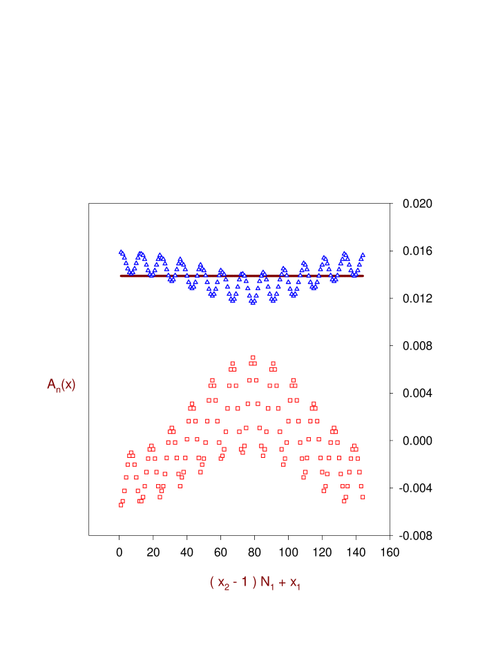
Figure 1: The anomaly function on a $12\times 12$ lattice. The background gauge field has constant field tensor with topological charge $Q=1$. The horizontal line at height $1/72$ is the Chern-Pontryagin density on the torus. The axial anomaly of $D$ [ Eq. (54) ] is denoted by triangles which fluctuate around the exact solution, while that of the Wilson-Dirac operator [ Eq. (51) with $m_{f}=0$ and $r_{w}=1$ ] by squares which are far away from the exact solution. The axial anomaly of $D^{\prime}$ [ Eq. (60) ] coincides with the exact solution ( the horizontal line at height $1/72$ ).

The non-locality of $D$ can be easily seen by plotting $D(x,y)$ as a function of $|x-y|$. In Fig. 2, one of the Dirac components of $|D(x,0)|$, say, $|D_{11}(x,0)|$ is plotted versus the distance $|x|$, on a $12\times 12$ lattice with periodic boundary conditions, in a constant background gauge field with topological charge $Q=1$. It is obvious that $D(x,y)$ is nonlocal.

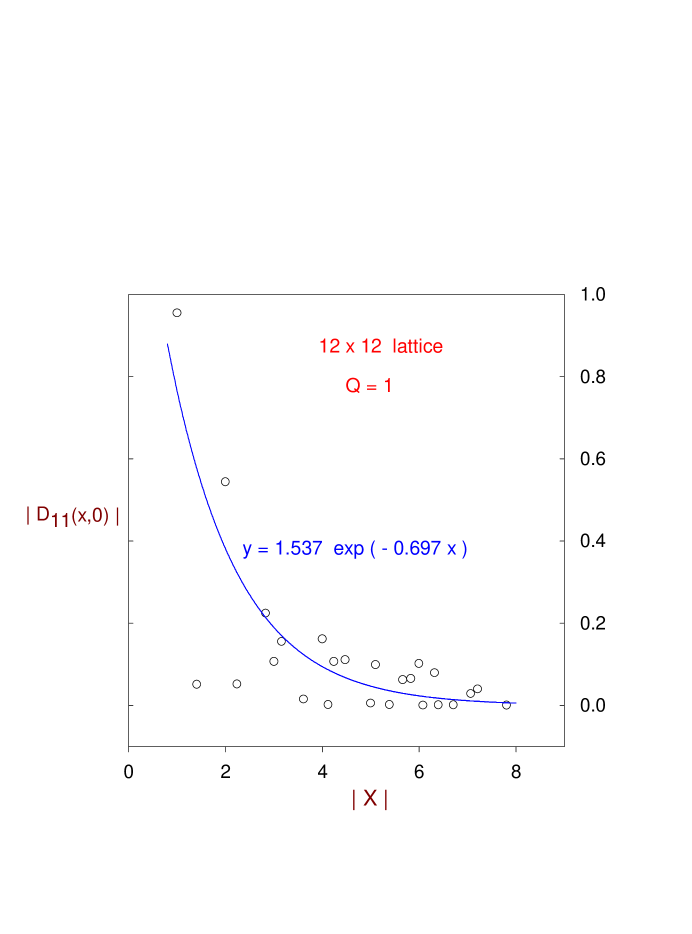
Figure 2: One of the Dirac components of $D(x,0)$, $|D_{11}(x,0)|$, is plotted as a function of $|x|$. The lattice is $12\times 12$ with periodic boundary conditions. The background gauge field has constant field tensor with topological charge $Q=1$. All data points with the same distance $|x|$ from the origin have been averaged. The solid line is an exponential fit to the data points.

Although $D$ is topologically proper, the non-locality of $D$ must yield incorrect chiral anomaly and fermion determinant. In Table 2, we compute the fermion determinant of $D$ for different topological sectors of constant field tensor, and compare them with the exact solution on a torus [30],

$$\mbox{det}_{1}[D(Q)]_{exact}=N\sqrt{\left({L_{1}L_{2}\over 2|Q|}\right)^{|Q|}}$$ (59)

where the zero modes have been omitted and the normalization constant is fixed by $N=\sqrt{{2\over L_{1}L2}}$ such that $\mbox{det}_{1}[D(1)]_{exact}=1$. It is evident that the fermion determinant of $D$ ( in the third coluum ) disagrees with the exact solution ( in the second coluum ), while those of a local $D^{\prime}$ [ Eq. (60) ] ( in the fourth coluum ) agree fairly well with the exact solutions. The fermion determinants for the Wilson-Dirac operator are listed in the fifth coluum, where all eigenvalues of $D_{w}$ are taken into account. Thus its fermion determinant must become smaller for larger $Q$ due to the emergence of small real eigenvalues. If we discard these small real eigenvalues of $D_{w}$, which correspond to the exact zero modes of $D$, then the resulting fermion determinant of $D_{w}$ is listed in the last coluum of Table 2, but still in disagreement with the exact solution. In general, the fermion determinant ratio of $D_{w}$ between any two gauge configurations ( no matter within the same topological sector, or in two different sectors ) disagrees with the exact solution, except for the trivial sector with $Q=0$.

Q	$\mbox{det}_{1}[D(Q)]_{exact}$	$\mbox{det}_{1}[D(Q)]$	$\mbox{det}_{1}[D^{\prime}(Q)]$	$\mbox{det}[D_{w}(Q)]$	$\mbox{det}^{\prime}[D_{w}(Q)]$
1	1.00000	1.00000	1.00000	1.00000	1.00000
2	4.24264	5.21339	4.22458	0.34182	3.98005
3	13.8564	23.5281	13.7284	0.14620	11.8619
4	38.1838	98.6168	37.2195	0.07092	28.8108
5	92.7342	394.114	90.3215	0.03841	61.1240
6	203.647	1535.83	198.435	0.02185	112.466
7	411.296	5759.04	391.581	0.01337	190.058
8	773.221	21275.2	726.985	0.00854	293.285

Table 2: The fermion determinant versus the topological charge $Q$. The exact solution for a torus of size $12\times 12$ is listed in the second coluum, which is computed according to Eq. (59). The normalization constants are fixed by the first row in each case. The lattice Dirac operators $D$, $D^{\prime}$ and $D_{w}$ are defined in Eqs. (54), (60) and (51) respectively.

As long as we have a topologically proper $D$, we can use the topologically invariant transformation (1) to obtain a local $D^{\prime}$ such that the anomaly function and the fermion determinant both agree with the exact solutions for smooth gauge configurations. For simplicity, we fix $R=r\mbox{1I}$ in (1). Note that there is a large range of $r$ values to render $D^{\prime}$ local for constant background gauge fields. For instance, we can pick $r=0.5$, then (1) gives

$$D^{\prime}=10\left(\sqrt{D_{w}^{\dagger}D_{w}}+D_{w}\right)\left(11\sqrt{D_{w}^{\dagger}D_{w}}+D_{w}\right)^{-1}$$ (60)

It is easy to check that $D^{\prime}$ is local by plotting $|D^{\prime}(x,y)|$ versus $|x-y|$, as shown in Fig. 3. The chiral anomaly and fermion determinant of $D^{\prime}$ agree very well with the exact solutions, as listed in Table 1 and Table 2.

Now we can introduce local fluctuations to the field tensor through the sinusoidal terms in Eqs. (72) and (73). For $Q=1$, $h_{1}=0.1$, $h_{2}=0.2$, $A_{1}^{(0)}=0.3$, $A_{2}^{(0)}=0.4$ and $n_{1}=n_{2}=1$ on a $12\times 12$ lattice, the anomaly function of $D^{\prime}$ is computed and compared with the Chern-Pontryagin density on the torus, as shown in Fig. 4. It is evident that $A_{n}(x)$ agress with $A_{c}(x)$ very well at each site.

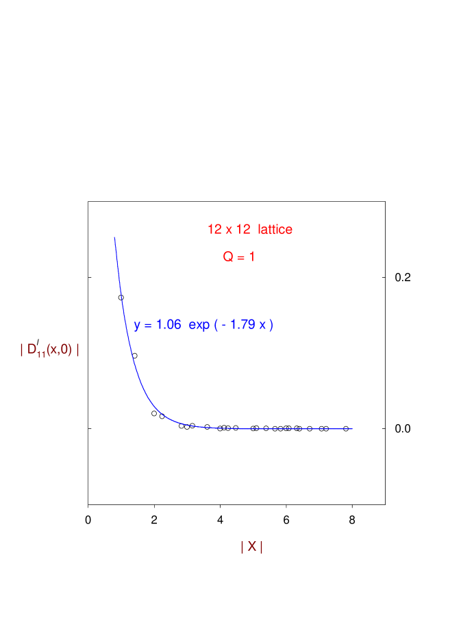
Figure 3: $|D^{{}^{\prime}}_{11}(x,0)|$ is plotted as a function of $|x|$. The lattice is $12\times 12$ with periodic boundary conditions. The constant background gauge field has topological charge $Q=1$. All data points at the same distance $|x|$ from the origin have been averaged. The solid line is an exponential fit to the data points. The same decay constant also fits very well for all other Dirac components of $D(x,y)$ and for any reference point $y$.

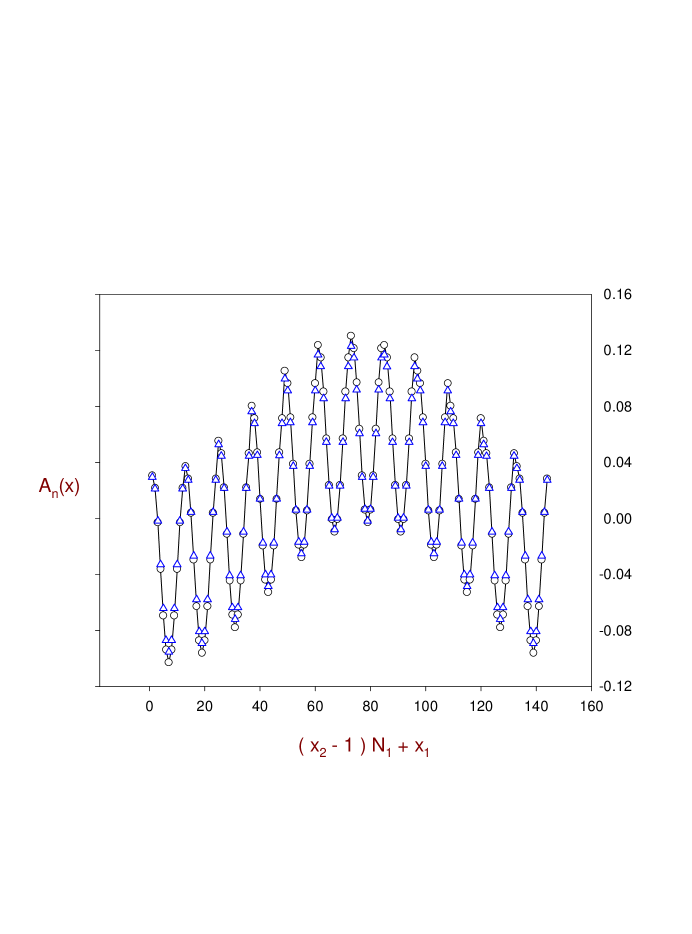
Figure 4: The anomaly function of $D^{\prime}$ [ Eq. (60) ] on a $12\times 12$ lattice versus the Chern-Pontryagin density ${\cal A}_{c}(x)$ [ Eq. (57) ] on the torus. The parameters of the background gauge field are $Q=1$, $h_{1}=0.1$, $h_{2}=0.2$, $A_{1}^{(0)}=0.3$, $A_{2}^{(0)}=0.4$ and $n_{1}=n_{2}=1$. The Chern-Pontryagin density is denoted by circles which are connected by line segments for the visual purpose. The anomaly function of $D^{\prime}$ is denoted by triangles.

Next we consider another lattice Dirac operator $D^{\prime\prime}$ which has the same form of $D^{\prime}$ (60) except $m_{0}=0.1$ in the $D_{w}$,

$$D^{\prime\prime}=10\left(\sqrt{D_{w}^{\dagger}D_{w}}+D_{w}\right)\left(11\sqrt{D_{w}^{\dagger}D_{w}}+D_{w}\right)^{-1}$$ (61)

where

$$D_{w}=-0.1+{1\over 2}[\gamma_{\mu}(\nabla\kern-0.5pt\smash{\raise 4.5pt\hbox{$\ast$}}\kern-4.5pt_{\mu}+{\nabla_{\mu}})-\nabla\kern-0.5pt\smash{\raise 4.5pt\hbox{$\ast$}}\kern-4.5pt_{\mu}{\nabla_{\mu}}]\ .$$

Again we investigate the properties of $D^{\prime\prime}$ in a background gauge field of constant field tensor. Then we find that $D^{\prime\prime}$ does not have any zero modes for $Q\geq 5$, in contrast to the behaviors of $D$ and $D^{\prime}$ having zero modes satisfying the Atiyah-Singer index theorem. In terms of the general index theorem, Eq. (27), we list the topological characteristics of $D$, $D^{\prime}$ and $D^{\prime\prime}$ in Table 3. It shows clearly that $c[D^{\prime\prime}]$ depends on the gauge configuration through $D^{\prime\prime}$. Note that $D$ is nonlocal for $Q=1$ to $Q=8$, but the Atiyah-Singer index theorem is still satisfied. We recall that the nonlocal $D$ and the local $D^{\prime}$ are related by the topological invariant transformation (1) which preserves the zero modes as well as the index.

Q	$c[D]$	$c[D^{\prime}]$	$c[D^{\prime\prime}]$
1	1	1	1
2	1	1	1
3	1	1	1
4	1	1	1
5	1	1	0
6	1	1	0
7	1	1	0
8	1	1	0

Table 3: The topological characteristics of $D$, $D^{\prime}$ and $D^{\prime\prime}$ versus the topological charge $Q$ on a $12\times 12$ lattice.

Now we introduce local fluctuations to the field tensor through the sinusoidal term in Eq. (72). Starting with constant field tensor at $Q=4$, we gradually increase the amplitude of the sinusoidal term, $A_{1}^{(0)}$ with $n_{2}=1$. The results are shown in Table 4. For $A_{1}^{(0)}\leq 0.0802$, the index of $D^{\prime\prime}$ is 4, satisfying the Atiyah-Singer index theorem. However, around $A_{1}^{(0)}=0.0803$, the index of $D^{\prime\prime}$ becomes $3$, thus the index theorem (27) is violated for any integer $c[D^{\prime\prime}]$. Therefore, we deduce that, in general, if $c[D]$ is not a constant for any integer topological charge $Q$, we can generalize $c[D]$ to a rational number, then the index theorem (27) also holds for any rough gauge fields. It is remarkable that the index of $D^{\prime\prime}$ changes so abruptly around $A_{1}^{(0)}=0.0802\sim 0.0803$, a singular behavior characterizes the topological phase transition. It is very unimaginable for us to see odd number of zero modes ( $N_{-}=3$ ) in a background gauge field of even number of topological charges ( $Q=4$ ). The underlying nonperturbative mechanism is very intriguing, and might have many unexpected consequences.

We note in passing that if we substitute $D^{\prime}$ [ Eq. (60) ] and $D^{\prime\prime}$ [ Eq. (61) ] by the Neuberger-Dirac operator $D_{h}=\mbox{1I}+D_{w}(D_{w}^{\dagger}D_{w})^{-1/2}$ with $m_{0}=1$ and $m_{0}=0.1$ respectively. The essential features of above numerical results are almost the same. In particular, the good agreement between the anomaly function and the Chern-Pontryagin density at each site, as shown in Fig. 4. We also note that the geometrical aspects of chiral anomalies in the overlap was investigated by Neuberger [31].

Q	$A_{1}^{(0)}$	$N_{-}-N_{+}$	$c[D^{\prime\prime}]$
4	0.0100	4	1
4	0.0200	4	1
4	0.0400	4	1
4	0.0600	4	1
4	0.0800	4	1
4	0.0801	4	1
4	0.0802	4	1
4	0.0803	3	3/4
4	0.0804	3	3/4
4	0.0810	3	3/4
4	0.0820	3	3/4
4	0.0900	3	3/4

Table 4: The topological characteristics of $D^{\prime\prime}$ versus the amplitude of the local sinusoidal fluctuation on a $12\times 12$ lattice, where $c[D^{\prime\prime}]$ is obtained in accordance with the general index theorem (27).

5 Summary and Discussions

In summary, we have shown that the condition for lattice Dirac operator $D$ ( or $D^{\prime}=D(\mbox{1I}+RD)^{-1}$ ) to reproduce the continuum anomaly function at each site of a finite lattice for smooth background gauge fields is that $D$ possesses exact zero modes satisfying the Atiyah-Singer index theorem ( i.e., $D$ is topologically proper ). This is the basic requirement for any Dirac operator to be used for lattice QCD if one wishes to reproduce correct chiral anomaly and fermion determinant ( ratio ) on a finite lattice. It is evident that the standard Wilson-Dirac fermion operator does not meet this basic requirement. If $D$ is topologically proper but nonlocal, then one can try to use (1) to transform $D$ into a local $D^{\prime}=D(\mbox{1I}+RD)^{-1}$ such that the anomaly function of $D^{\prime}$ agrees with the Chern-Pontryagin density in continuum. Note that there is no need for fine-tunings of $R$. The set of transformations $\{{\cal T}(R)\}$ defined in (1) form an abelian group with the group parameter space $\{R\}$. It is evident that (1) is one of the simplest topologically invariant transformations which preserve the zero modes and the index of $D$.

The chiral anomaly on the lattice can be understood from two seemingly different viewpoints. In general, if we have lattice Dirac operator $D$ which breaks the usual chiral symmetry according to Eq. (11), then the chiral anomaly can be obtained through the chiral symmetry breaking term [ Eq. (25 ], while the fermion measure is invariant under the usual chiral transformation, in contrast to the continuum theory in which the non-invariance of the fermion measure under the chiral transformation leads to the emergence of chiral anomaly after regularization [32]. Another viewpoint to understand the chiral anomaly on a finite lattice is only for those $D$ having chirally symmetric limit $D_{c}$ under the transformation (1). Then $D$ satisfies the Ginsparg-Wilson relation (10) which is the lattice chiral symmtry, thus the lattice action is invariant under the lattice chiral transformation. However, the fermionic measure is not invariant under the lattice chiral transformation, and thus leads to the chiral anomaly [20], reminiscent of the situation in continuum. Therefore, for Ginsparg-Wilson Dirac operator, one must obtain the same anomaly function (33) no matter which viewpoint one prefers. However, Eqs. (25) and (31) are the general formulas of the anomaly function for any lattice Dirac operator.

There is a vital difference between the continuum Dirac operator and the lattice ones. In continuum, the Dirac operator in a smooth non-trivial gauge background must have exact zero modes satisfying the Atiyah-Singer index theorem. On the other hand, lattice Dirac operator does not necessarily possess exact zero modes in a smooth non-trivial gauge background, not to mention satisfying the Atiyah-Singer index theorem. This naturally leads to the concept of topological characteristics, $c[D]$, which is an intrinsic attribute of $D$, in general, is not entirely due to the non-locality of $D$ and/or the occurrence of species doubling. Even if one starts with a lattice Dirac operator $D$ which is local and free of species doubling in a constant background gauge field, and the zero modes of $D$ also satisfies the Atiyah-Singer index theorem. However, as we increase the topological charge or the local fluctuations of the background gauge field, $D$ may undergo a topological phase transition and its zero modes may violate the Atiyah-Singer index theorem. In fact $D$ has become nonlocal long before it reaches the topological phase transition point. So, the non-locality of $D$ cannot be the crucial factor for violations of the Atiyah-Singer index theorem, though it explains the breakdown of the anomaly function (29) unambiguously. If one tries to explain the violations of Atiyah-Singer index theorem in terms of species doubling, then one has great difficulties to explain the occurrence of odd number of zero modes in a gauge background of even number of topological charges, as shown in Table 4. Therefore we conclude that the topological characteristics of lattice Dirac operator $D$ is a basic attribute of $D$, which in general is a rational number appearing in the general index theorem (27) for integer topological charge $Q$.

Given a lattice Dirac operator $D$, we cannot gaurantee that for any gauge configuration, there exists an operator $R$ such that the topologically invariant transformation (1) gives a local and smooth $D^{\prime}$. The notion of locality is usually defined as follows : $|D(x,y)|\sim\exp(-M|x-y|/a)$ with $M=O(1)$, or $|D(x,y)|=0$ for $|x-y|>d$ with $d=O(a)$. Although $|D(x,y)|$ can be fitted by $\exp(-M|x-y|/a)$ with $M=O(1)$, it may turn out that $|D(x,y)|$ is still highly fluctuating and/or anisotropic. So, it is necessary to introduce the notion of ”smoothness” which measures the fluctuations of $|D(x,y)|$ with respect to $\exp(-M|x-y|/a)$. To determine the criterion for the gauge configuration such that $D^{\prime}$ is local and smooth is beyond the scope of the present paper. It is apparent that such criterion should take into account of the fluctuations between the plaquettes as well as the deviations of each plaquette from the identity. Otherwise the criterion is only useful in the weak field limit. For example, the Neuberger-Dirac operator $D_{h}$ with $m_{0}=r_{w}=1$ and $D^{\prime}$ [ Eq. (60) ] are both local and smooth for gauge configurations with constant field tensors up to very large $Q$ values ( see Table 3 ), though each plaquette is very different from the identity. If one takes into account of the degree of freedom provided by the transformation (1), then the criterion for a smooth gauge configuration could be less stringent than without it.

A scheme for dynamical fermion simulation of lattice QCD is outlined in Section 3. Since the direct computation of fermion determinant is prohibitively expensive for lattice QCD, a practical implementation of the scheme must be worked out before we can proceed to any realistic calculations. Nevertheless, the prescription of decomposing link configurations into distinct topological sectors and performing Monte Carlo simulations for each relevant topological sector individually may open new avenues to tackle the longstanding problems in QCD.

Appendix A

In this appendix, we give an example of prescribed background gauge field which has been used in ref. [25, 12] for two dimensional and four dimensional lattices respectively. On a 4-dimensional torus ( $x_{\mu}\in[0,L_{\mu}],\mu=1,\cdots,4$ ), the simplest nontrivial gauge fields can be represented as

$$A_{1}(x) = t^{a}\left[{2\pi h_{1}\over L_{1}}-{2\pi q_{1}x_{2}\over L_{1}L_{2}}+A_{1}^{(0)}\sin\left({2\pi n_{2}\over L_{2}}x_{2}\right)\right]$$ (63)

$$A_{2}(x) = t^{a}\left[{2\pi h_{2}\over L_{2}}+A_{2}^{(0)}\sin\left({2\pi n_{1}\over L_{1}}x_{1}\right)\right]$$ (64)

$$A_{3}(x) = t^{a}\left[{2\pi h_{3}\over L_{3}}-{2\pi q_{2}x_{4}\over L_{3}L_{4}}+A_{3}^{(0)}\sin\left({2\pi n_{4}\over L_{4}}x_{4}\right)\right]$$ (65)

$$A_{4}(x) = t^{a}\left[{2\pi h_{4}\over L_{4}}+A_{4}^{(0)}\sin\left({2\pi n_{3}\over L_{3}}x_{3}\right)\right]$$ (66)

where $t^{a}$ is any one of the generators of the gauge group with the normalization $\mbox{tr}(t^{a}t^{b})=n\ \delta^{ab}$, and $q_{1}$ and $q_{2}$ are integers. The global part is characterized by the topological charge

$$Q={1\over 32\pi^{2}}\int d^{4}x\ \epsilon_{\mu\nu\lambda\sigma}\ \mbox{tr}(F_{\mu\nu}F_{\lambda\sigma})=n\ q_{1}\ q_{2}$$ (67)

which is an integer. The harmonic parts are parameterized by four real constants $h_{1}$, $h_{2}$, $h_{3}$ and $h_{4}$. The local parts are chosen to be sinusoidal fluctuations with amplitudes $A_{1}^{(0)}$, $A_{2}^{(0)}$, $A_{3}^{(0)}$ and $A_{4}^{(0)}$, and frequencies ${2\pi n_{2}\over L_{2}}$, ${2\pi n_{1}\over L_{1}}$, ${2\pi n_{4}\over L_{4}}$ and ${2\pi n_{3}\over L_{3}}$ where $n_{1}$, $n_{2}$, $n_{3}$ and $n_{4}$ are integers. The discontinuity of $A_{1}(x)$ ( $A_{3}(x)$ ) at $x_{2}=L_{2}$ ( $x_{4}=L_{4}$ ) due to the global part only amounts to a gauge transformation. The field tensors $F_{12}$ and $F_{34}$ are continuous on the torus, while other $F^{\prime}s$ are zero.

To transcribe the continuum gauge fields to the lattice, we take the lattice sites at $x_{\mu}=0,a,...,(N_{\mu}-1)a$, where $a$ is the lattice spacing and $L_{\mu}=N_{\mu}a$ is the lattice size. Then the link variables are

$$U_{1}(x) = \exp\left[{\hbox{\rm i}}A_{1}(x)a\right]$$ (68)

$$U_{2}(x) = \exp\left[{\hbox{\rm i}}A_{2}(x)a+{\hbox{\rm i}}\delta_{x_{2},(N_{2}-1)a}{2\pi q_{1}x_{1}\over L_{1}}\ t^{a}\right]$$ (69)

$$U_{3}(x) = \exp\left[{\hbox{\rm i}}A_{3}(x)a\right]$$ (70)

$$U_{4}(x) = \exp\left[{\hbox{\rm i}}A_{4}(x)a+{\hbox{\rm i}}\delta_{x_{4},(N_{4}-1)a}{2\pi q_{2}x_{3}\over L_{3}}\ t^{a}\right]$$ (71)

The last term in the exponent of $U_{2}(x)$ ( $U_{4}(x)$ ) is included to ensure that the field tensor $F_{12}$ ( $F_{34}$ ) which is defined by the ordered product of link variables around a plaquette is continuous on the torus. For $U(1)$ gauge field on a two-dimensional lattice, the link variabes are reduced to Eqs. (68) and (69) with

$$A_{1}(x) = {2\pi h_{1}\over L_{1}}-{2\pi Qx_{2}\over L_{1}L_{2}}+A_{1}^{(0)}\sin\left({2\pi n_{2}\over L_{2}}x_{2}\right)$$ (72)

$$A_{2}(x) = {2\pi h_{2}\over L_{2}}+A_{2}^{(0)}\sin\left({2\pi n_{1}\over L_{1}}x_{1}\right)$$ (73)

where the topological charge is

$$Q={1\over 2\pi}\int d^{2}x\ F_{12}$$ (74)

Acknowledgement

This work was supported by the National Science Council, R.O.C. under the grant number NSC88-2112-M002-016.

References

- [1] S. Adler, Phys. Rev. 177 (1969) 2426; J.S. Bell and R. Jackiw, Nuovo Cimento 60 (1969) 47.
- [2] G ’t Hooft, Phys. Rev. Lett. 37 (1976) 8; Phys. Rev. D17 (1976) 3432; Phys. Rep. 142 (1986) 357.
- [3] For a detailed account and references, see, e.g., S. Weinberg, The Quantum Theory of Fields, vol. II, ( Cambridge University Press, 1996).
- [4] T.W. Chiu and S.V. Zenkin, Phys. Rev. D59, 074501 (1999).
- [5] K. G. Wilson, in New Phenomena in Subnuclear Physics, proceedings of the 14th course of the International School of Subnuclear Physics, Erice, 1975, edited by A. Zichichi ( Plenum, New York, 1977 ); K. G. Wilson, Phys. Rev. D 10 (1974) 2445.
- [6] H.B. Nielsen and N. Ninomiya, Nucl. Phys. B185, 20 (1981); B193, 173 (1981).
- [7] T.W. Chiu, Phys. Lett. B445 (1999) 371.
- [8] P. Ginsparg and K. Wilson, Phys. Rev. D 25 (1982) 2649.
- [9] H. Neuberger, Phys. Lett. B417 (1998) 141; Phys. Lett. B427 (1998) 353.
- [10] P. Hasenfratz, Nucl. Phys. B525 (1998) 401.
- [11] S. Chandrasekharan, ”Lattice QCD with Ginsparg-Wilson fermion”, hep-lat/9805015.
- [12] T.W. Chiu, ”Topological phases in Neuberger-Dirac operator”, hep-lat/9810002.
- [13] T.W. Chiu and T.H. Hsieh, ”Perturbation calculation of the axial anomaly of Ginsparg-Wilson fermion”, hep-lat/9901011.
- [14] M. Lüscher, Nucl. Phys. B538 (1999) 515.
- [15] Y. Kikukawa and A. Yamada, Phys. Lett. B 448, 265 (1999).
- [16] K. Fujikawa, Nucl. Phys. B546, 480 (1999).
- [17] D. Adams, ”Axial anomaly and topological charge in lattice gauge theory with overlap-Dirac operator”, hep-lat/9812003.
- [18] H. Suzuki, ”Simple evaluation of chiral Jacobian with overlap-Dirac operator”, hep-th/9812019.
- [19] P. Hasenfratz, V. Laliena and F. Niedermayer, Phys. Lett. B427 (1998) 125.
- [20] M. Lüscher, Phys. Lett B 428 (1998) 342.
- [21] C. Callan, R. Dashen and D. Gross, Phys. Lett. 63B, 334 (1976); R. Jackiw and C. Rebbi, Phys. Rev. Lett. 37, 172 (1976).
- [22] R. Narayanan and H. Neuberger, Nucl. Phys. B443, 305 (1995).
- [23] D.B. Kaplan, Phys. Lett. B288, 342 (1992).
- [24] S.A. Frolov and A.A. Slavnov, Phys. Lett. B309, 344 (1993).
- [25] T.W. Chiu, Phys. Rev. D58 (1998) 074511.
- [26] L.H. Karsten and J. Smit, Nucl. Phys. B183, 103 (1981).
- [27] W. Kerler, Phys. Rev. D 23, 2384 (1981).
- [28] E. Seiler and I.O. Stamatescu, Phys. Rev. D25, 2177 (1982); erratum: D26, 534 (1982).
- [29] K. Fujikawa, Z. Phys. C25, 179 (1984).
- [30] I. Sachs and A. Wipf, Helv. Phys. Acta 65, 652 (1992).
- [31] H. Neuberger, Phys. Rev. D 59, 085006 (1999).
- [32] K. Fujikawa, Phys. Rev. Lett. 42, 1195 (1979).