We study the dual Higgs theory for the confinement mechanism based on Quantum Chromodynamics (QCD) in the ’t Hooft abelian gauge. In the abelian gauge, QCD is reduced into an abelian gauge theory including color-magnetic monopoles, which appear corresponding to the nontrivial homotopy group $\Pi_{2}($SU$(N_{c})/$U$(1)^{N_{c}-1})$ $={\bf Z}^{N_{c}-1}$. With the two conjectures of abelian dominance and monopole condensation, QCD in the abelian gauge becomes the dual Higgs theory, and then color confinement can be understood as one-dimensional squeezing of the color-electric flux due to the dual Meissner effect. In the basis of the dual superconductor picture, confinement phenomena are systematically studied using the lattice QCD Monte-Carlo simulation, the monopole-current dynamics and the dual Ginzburg-Landau (DGL) theory, an infrared effective theory of QCD.

First, we study the origin of abelian dominance for the confinement force in the maximally abelian (MA) gauge in terms of the gluon-field properties using the lattice QCD. In the MA gauge, the gluon-field fluctuation is maximally concentrated in the abelian sector. As the remarkable feature in the MA gauge, the amplitude of the off-diagonal gluon is strongly suppressed, and therefore the phase variable of the off-diagonal (charged) gluon tends to be random, according to the weakness of the constraint from the QCD action. Using the random-variable approximation for the charged-gluon phase variable, we find the perimeter law of the charged-gluon contribution to the Wilson loop and show abelian dominance for the string tension in the semi-analytical manner. These theoretical results are also numerically confirmed using the lattice QCD simulation.

Second, we study the QCD-monopole appearing in the abelian sector in the abelian gauge. The appearance of monopoles is transparently formulated in terms of the gauge connection, and is originated from the singular nonabelian gauge transformation to realize the abelian gauge. We investigate the gluon field around the monopole in the lattice QCD. The QCD-monopole carries a large fluctuation of the gluon field and provides a large abelian action of QCD. Nevertheless, QCD-monopoles can appear in QCD without large cost of the QCD action, due the large cancellation between the abelian and off-diagonal parts of the QCD action density around the monopole. We derive a simple relation between the confinement force and the monopole density by idealizing the monopole contribution to the Wilson loop.

Third, we study the monopole-current dynamics using the infrared monopole-current action defined on a lattice. We adopt the local current action, considering the infrared screening of the inter-monopole interaction due to the dual Higgs mechanism. When the monopole self-energy $\alpha$ is smaller then $\alpha_{c}=$ ln$(2D-1)$, monopole condensation can be analytically shown, and we find this system being in the confinement phase from the Wilson loop analysis. By comparing the lattice QCD with the monopole-current system, the QCD vacuum is found to correspond to the monopole-condensed phase in the infrared scale. We consider the derivation of the DGL theory from the monopole ensemble, which would be essence of the QCD vacuum in the MA gauge because of abelian dominance and monopole dominance.

Finally, we study the QCD phase transition at finite temperatures in the DGL theory. We formulate the effective potential at various temperatures in the imaginary-time formalism. Thermal effects reduce the QCD-monopole condensate and bring a first-order deconfinement phase transition. We find a large reduction of the self-interaction among QCD-monopoles and the glueball mass near the critical temperature by considering the temperature dependence of the self-interaction. The string tension is also calculated at finite temperatures. We apply also the DGL theory for the bubble formation process in early Universe and quark-gluon-plasma (QGP) formation process in the ultra-relativistic heavy-ion collision.

Chapter 1 Introduction

Quantum Chromodynamics (QCD) is the fundamental theory of the strong interaction, and describes the properties and the underlying structure of hadrons in terms of quarks and gluons. The QCD Lagrangian has the local SU($N_{c}$) symmetry and is written by the quark $q$ and the gluon field $A_{\mu}$ as

$${\cal L}_{\rm QCD}=-\frac{1}{2}{\rm tr}\left(G_{\mu\nu}G^{\mu\nu}\right)+\bar{q}\left(i\gamma_{\mu}D^{\mu}-m\right)q,$$ (1.1)

where $G_{\mu\nu}$ is the SU($N_{c}$) field strength $G_{\mu\nu}\equiv\frac{1}{ie}[{\hat{D}_{\mu}},{\hat{D}_{\nu}}]$ and $\hat{D}_{\mu}$ is covariant-derivative $\hat{D}_{\mu}=\hat{\partial}_{\mu}+ieA_{\mu}$ [1, 2, 3]. In the chiral limit $m\to 0$ with $N_{f}$ flavor, this Lagrangian has also global chiral symmetry U($N_{f}$)_L $\times$ U($N_{f}$)_R, although U(1)_A is explicitly broken by the U(1)_A anomaly at the quantum level [1].

Due to the asymptotic freedom, the gauge-coupling constant of QCD becomes small in the high-energy region and the perturbative QCD provides a direct and systematic description of the QCD system in terms of quarks and gluons. On the other hand, in the low-energy region, the strong gauge-coupling nature of QCD leads to nonperturbative features like color confinement, dynamical chiral-symmetry breaking [4, 5, 6] and nontrivial topological effect by instantons [7, 8, 9], and it is hard to understand them directly from quarks and gluons in a perturbative manner. Instead of quarks and gluons, some collective or composite modes may be relevant degrees of freedom for the nonperturbative description in the infrared region of QCD. As for chiral dynamics, the pion and the sigma meson play the important role for the low-energy QCD, and they are included in the effective theory like the (non-) linear sigma model [1, 10], the chiral bag model [11, 12] and the Nambu-Jona-Lasinio model [13, 14], where these mesons are described as composite modes of quarks. Here, the pion is considered to be the Nambu-Goldstone boson relating to spontaneous chiral-symmetry breaking and obeys the low-energy theorem and the current algebra [1]. On the other hand, confinement is essentially described by dynamics of gluons rather than quarks. Hence, it is quite desired to extract the relevant collective mode from gluon for confinement phenomena.

In 1970’s, Nambu, ’t Hooft and Mandelstam proposed an interesting idea that quark confinement can be interpreted using the dual version of the superconductivity [15, 16, 17] (see Fig.1.1). In the ordinary superconductor, Cooper-pair condensation leads to the Meissner effect, and the magnetic flux is excluded or squeezed like a quasi-one-dimensional tube as the Abrikosov vortex, where the magnetic flux is quantized topologically. On the other hand, from the Regge trajectory of hadrons and the lattice QCD, the confinement force between the color-electric charge is characterized by the universal physical quantity of the string tension, and is brought by one-dimensional squeezing of the color-electric flux [18] in the QCD vacuum. Hence, the QCD vacuum can be regarded as the dual version of the superconductor based on above similarities on the low-dimensionalization of the quantized flux between charges. In this dual-superconductor picture for the QCD vacuum, as the result of condensation of color-magnetic monopoles, which is the dual version of the electric charge, the squeezing of the color-electric flux between quarks is realized by the dual Meissner effect. However, there are two following large gaps between QCD and the dual superconductor picture.

1. This picture is based on the abelian gauge theory subject to the Maxwell-type equations, where electro-magnetic duality is manifest, while QCD is a nonabelian gauge theory.

2. The dual-superconductor scenario requires condensation of (color-) magnetic
   monopoles as key concept, while QCD does not have such a monopole as the elementary degrees of freedom.

As the connection between QCD and the dual superconductor scenario, ’t Hooft proposed concept of the abelian gauge fixing [19], the partial gauge fixing which only remains abelian gauge degrees of freedom in QCD. By definition, the abelian gauge fixing reduces QCD into an abelian gauge theory, where the off-diagonal element of the gluon field behaves as a charged matter field and provides a color-electric current in terms of the residual abelian gauge symmetry. As a remarkable fact in the abelian gauge, color-magnetic monopole appears as topological object corresponding to nontrivial homotopy group $\Pi_{2}({\rm SU}(N_{c})/$U$(1)^{N_{c}-1})={\bf Z}^{N_{c}-1}_{\infty}$. Thus, by the abelian gauge fixing, QCD is reduced into an abelian gauge theory including both the electric current $j_{\mu}$ and the magnetic current $k_{\mu}$, which is expected to provide a theoretical basis of the monopole-condensation scheme for the confinement mechanism.

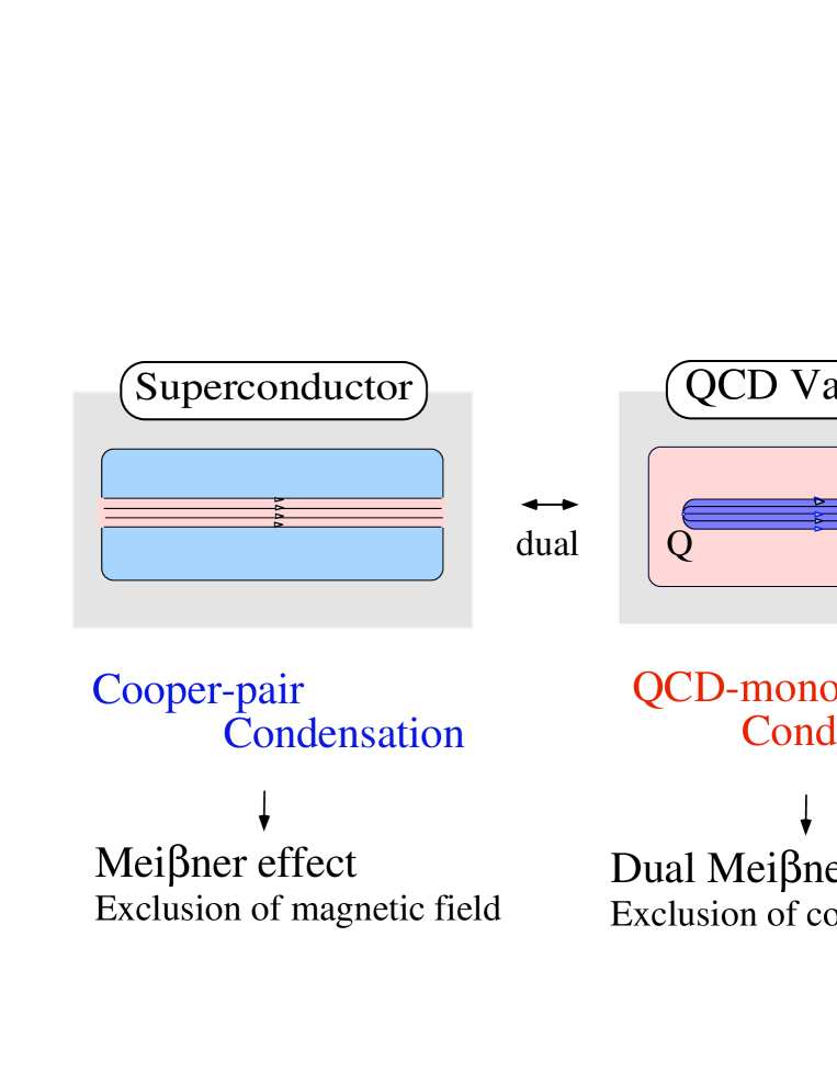
Figure 1.1: Correspondence of the QCD vacuum to the superconductor. In the QCD vacuum, the color confinement is realized by monopole condensation. In the superconductor, the Meissner effect occurs by Cooper-pair condensation.

For irrelevance of the off-diagonal gluons, Ezawa and Iwazaki assumed abelian dominance that the only abelian gauge fields with monopoles would be essential for the description of nonperturbative phenomena in the low-energy region of QCD, and showed a possibility of monopole condensation in an infrared scale by investigating “energy-entropy balance” on the monopole current [20] in a similar way to the Kosterlitz-Thouless transition in the 1+2 dimensional superconductivity [21]. Ezawa and Iwazaki formulated the dual London theory as an infrared effective theory of QCD, and later Maedan and Suzuki reformulated it as the dual Ginzburg-Landau (DGL) theory in 1988 [22].

Furthermore, such abelian dominance and monopole condensation have been investigated using the lattice QCD simulation in the maximally abelian (MA) gauge [23, 24, 25, 26]. The MA gauge is the abelian gauge where the diagonal component of gluon is maximized by the gauge transformation. In the MA gauge, physical information of the gauge configuration is concentrated into the diagonal components as much as possible. The lattice QCD studies indicate abelian dominance that the string tension [25, 26, 27] and chiral condensate [28, 29] are almost described only by abelian variables in the MA gauge. In the lattice QCD, monopole dominance is also observed such that only the monopole part in the abelian variable contributes to the nonperturbative QCD in the MA gauge [28, 30]. Thus, the lattice QCD simulations show strong evidence on the dual Higgs theory for the nonperturbative QCD in the MA gauge [31, 32].

As the result, DGL theory is expected as a reliable infrared effective theory of QCD. Recently, RCNP group studied the DGL theory [22, 33], and derived the simple formula for the string tension and also pointed out the relevant role of monopole condensation to chiral symmetry breaking by solving the Schwinger-Dyson equation with the nonperturbative gluon propagator [33, 34, 35]. This abelian dominance for chiral-symmetry breaking is confirmed by Miyamura and Woloshyn in more rigid framework of the lattice QCD [28, 29]. Considering the fact that instanton needs the nonabelian component for existence, RCNP group pointed out the correlation between instantons and monopoles in the abelian dominant system in terms of the remaining large off-diagonal component around the monopole, which is the topological defect. The evidence on the strong correlation between instantons and monopoles have been observed also in the lattice QCD calculation [36] and in the analytical demonstration using the Polyakov-like gauge [37, 38] and the MA gauge [39, 40]. Thus, the monopole seems to play the essential role for the nonperturbative QCD like confinement and chiral symmetry breaking and topology [31, 32, 41].

A question arises if the color is confined in the QCD vacuum by monopole condensation all the time? As the superconducting state at low temperature is changed into the normal phase at high temperature, the QCD vacuum would also change from the confinement phase to the quark-gluon-plasma (QGP) phase, where the quark and gluon can move freely. This phase transition is called QCD phase transition, and becomes one of the most important subject related to various fields such as the early Universe and relativistic heavy-ion collision. According to the big bang scenario, which is a successful model for cosmology, the quark gluon plasma phase at high temperature is changed into the hadron phase 10^-6 second after the big bang. At the Brookhaven National Laboratory in the United States, some physicists are trying to form the quark gluon plasma as a new matter by colliding high energy heavy-ions using RHIC. RCNP group also has studied the QCD vacuum at finite temperature in terms of confinement-deconfinement phase transition and chiral phase transition using the DGL theory.

In this way, the study of color confinement phenomena based on the dual Higgs picture is divided into two categories in terms of the method of approach.

1. Study with the lattice QCD, which is an useful method for the direct calculation of the QCD partition functional $Z_{\rm QCD}$ [42, 43].

2. Study with the infrared effective theory, the DGL theory [22, 33], which consists of the essential degrees of the freedom for infrared phenomena.

In the lattice formalism, space-time coordinate is discretized with the lattice spacing $a$, and the theory is described by the link variable $U_{\mu}(s)=e^{iaeA_{\mu}(s)}$, which corresponds to the line integral $P\exp\{i\int_{s}^{s+\hat{\mu}}dx_{\mu}eA_{\mu}(x)\}$ along the link. The lattice QCD partition functional $Z$ in the Euclidean metric is given as

$$Z=\int dU_{\mu}e^{-\beta\hat{S}[U_{\mu}]},$$ (1.2)

where $\beta\equiv\frac{2N_{c}}{e^{2}(a)}$ is the control parameter related to the lattice spacing $a$ [42] (Appendix A.1). Here, $e(a)$ is the QCD running coupling constant. The standard lattice action is given as

$$\hat{S}=\sum_{s,\mu>\nu}[1-\frac{1}{2N_{c}}{\rm tr}\{\Box_{\mu\nu}(s)+\Box^{\dagger}_{\mu\nu}(s)\}],$$ (1.3)

where $\Box_{\mu\nu}(s)$ is plaquette defined as

$$\Box_{\mu\nu}(s)\equiv U_{\mu}(s)U_{\nu}(s+\hat{\mu})U^{\dagger}_{\mu}(s+\hat{\nu})U_{\nu}^{\dagger}(s).$$ (1.4)

In the limit $a\rightarrow 0$, i.e. $\beta\rightarrow\infty$, and the lattice action $\beta\hat{S}$ becomes the QCD action $S_{\rm QCD}$ in the continuum theory. The gauge configuration of QCD is generated on the lattice using the Monte Carlo method (Appendix A.2). In the lattice QCD, the abelian gauge fixing can be performed after the generation of gauge configurations, and the abelian link variable is extracted by neglecting the off-diagonal part, which is called as the abelian projection. In the lattice formalism, the abelian link variable can be separated numerically into the photon part and the monopole part corresponding to the separation of the electric current and the monopole current as will be shown in Chapter 6. The dual-superconductor scenario for confinement has been examined in the lattice QCD by measurements of the abelian variable, monopole and so on in the abelian gauge.

On the other hand, the DGL theory is derived from the gluon sector of QCD, and is composed of the dual gauge field ${\cal B}_{\mu}$ and the monopole field $\chi$ in the pure gauge case. The Lagrangian is expressed as

$${\cal L}_{DGL}={\rm tr}{\hat{\cal L}}$$

$$\hat{\cal L}=-{1\over 2}(\partial_{\mu}{\cal B}_{\nu}-\partial_{\nu}{\cal B}_{\mu})^{2}+[\hat{D}_{\mu},\chi]^{{\dagger}}[\hat{D}_{\mu},\chi]-\lambda(\chi^{{\dagger}}\chi-v^{2})^{2},$$ (1.5)

where $\hat{D}_{\mu}=\hat{\partial}_{\mu}+ig{\cal B}_{\mu}$ is the dual covariant derivative. Imposing the abelian gauge fixing on QCD, the monopole appears as the line-like object in 4-dimensional space. The monopole field is derived by summing all the paths of the monopole trajectories and monopole-field interaction is introduced taking the lattice result “monopole condensation” into the consideration. Here, the off-diagonal component is neglected due to the lattice QCD result “abelian dominance”, and the dual gauge field ${\cal B}_{\mu}$ is used instead of the abelian gauge field $A_{\mu}$ adopting the Zwanziger formalism in order to describe gluon dynamics without the singularity in the gauge field.

The DGL theory provides an useful method of studying the various confinement phenomena such as inter-quark potential, hadron flux-tube system and the phase transition, since it gives not only just the numerical results on the various quantities but also their reasons. This is largely different from the lattice simulation. The quark-antiquark potential arises from the strong correlation between two quarks in the infrared region, which is revealed by the DGL gluon propagator with double pole. The hadron flux is constructed by a massive dual gauge field, whose mass is obtained by the dual Higgs mechanism of monopole condensation. However, in the process of the construction of DGL theory, abelian dominance and monopole condensation is assumed, and its origin is not clear. Namely, we can not answer the question what feature of the monopole degrees of freedom is important for such confinement phenomena or where the effect of nonabelian feature appears.

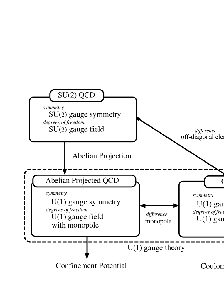
Figure 1.2: Comparison among QCD, abelian projected QCD (AP-QCD) and QED in terms of the gauge symmetry and fundamental degrees of freedom. ($N_{c}$ = 2)

In this paper, we try to understand the confinement mechanism based on the dual Higgs mechanism using both methods, the lattice QCD simulation and the DGL theory. In the first half of this paper, we study the origin of abelian dominance and monopole condensation in terms of the gluon configuration using the lattice QCD, and in the second half we apply the DGL theory to the confinement phenomena such as QCD phase transition and multi-hadron flux tube system.

The point at issue in the first half is the following three subjects.

1. What is the origin of abelian dominance for infrared quantities like the string tension in the MA gauge?

2. Why does monopole appear in abelian projected QCD(AP-QCD), although AP-QCD is an abelian gauge theory like QED?

3. What is the role of monopoles for the confinement phenomena? What is the role of the off-diagonal component of gluon in QCD in the MA gauge?

In the MA gauge, AP-QCD neglecting the off-diagonal gluon component almost reproduces essence of the nonperturbative QCD, although AP-QCD is an abelian gauge theory like QED. One may speculate that the strong-coupling nature leads to the similarity between AP-QCD and QCD, because the gauge coupling $e$ in AP-QCD [44] is the same as that in QCD in the lattice simulation. However, the strong-coupling nature would not be enough to explain the nonperturbative feature, because, if monopoles are eliminated from AP-QCD, nonperturbative features are lost in the remaining system called as photon part, although the gauge coupling $e$ is same as that in QCD. For further understanding, let us compare the theoretical structure of QCD, AP-QCD and QED in terms of the gauge symmetry and the fundamental degrees of freedom as shown in Fig.1.2. As for the interaction, the linear confinement potential arises both in QCD and in AP-QCD, while only the Coulomb potential appears in QED. On the symmetry, QCD has a nonabelian gauge symmetry, while both AP-QCD and QED have abelian gauge symmetry. The obvious difference between QCD and QED is existence of off-diagonal gluons in QCD. On the other hand, the difference between AP-QCD and QED is existence of the monopole, since the magnetic monopole does not exist in QED because of the Bianchi identity. This indicates the close relation between monopoles and off-diagonal gluons. In particular, off-diagonal gluon components play a crucial role for existence of the monopole [45], and the monopole itself is expected to play an alternative role of off-diagonal gluons for confinement.

In Chapter 2, we review the abelian gauge fixing in line with ’t Hooft to discuss the confinement phenomena in terms of the monopoles based on the dual superconductor picture. We show the gauge invariance condition in the abelian gauge. As the abelian gauge fixing, we introduce the maximally abelian gauge, which is considered to be the best abelian gauge for the infrared physics according to recent lattice QCD studies. In addition, we generalize the maximally abelian gauge fixing.

In Chapter 3, we investigate the origin of abelian dominance in the MA gauge in the SU(2) gauge theory. We introduce the abelian projection rate, which is defined as the overlapping factor between SU(2) link variable and abelian link variable, and investigate abelian dominance for the abelian link variable. We study abelian dominance for the Wilson loops in terms of by approximating the off-diagonal angle variable as a random variable. Using the U(1)₃ Landau gauge, we study the abelian gauge field and abelian field strength directly in the MA gauge. Then, we compare the abelian gauge field in the SU(2) Landau gauge, where the gauge field is fixed most continuously and study the feature of the MA gauge in terms of the gluon field fluctuation.

In Chapter 4, we investigate the mechanism of the appearance of monopole in AP-QCD both in the continuum theory and in the lattice QCD formalism. We show the appearance of monopole using the covariant derivative in the abelian sector of QCD, clarifying the role of the off-diagonal components of QCD.

In Chapter 5, we investigate the relations between monopoles and gauge-field fluctuations in the MA gauge, measuring the probability distribution of gluons around the monopole. We show the distribution of the action density on the SU(2), U(1)₃ and off-diagonal part around the monopoles and consider the appearance of the monopole in terms of the action density.

In Chapter 6, we study extraction of the monopole degrees of freedom from U(1)₃ gauge theory. The abelian gauge field is decomposed into the monopole and photon parts. We investigate the properties on the magnetic and electric currents, action density, field variable itself in both parts. We show the scaling properties on the monopole current and the Dirac sheet and obtain the good scaling on variables related to the Dirac sheet. Furthermore, we obtain the simple relation between the string tension and monopole current density.

In Chapter 7, we study monopole condensation in the QCD vacuum by comparing to the monopole-current system. We first generate the monopole-current system on the lattice using a simple monopole current action, and study the role of monopole current to confinement.

In the second part of this paper, making the best use of the DGL theory, we investigate the QCD phase transition using effective potential formalism, and multi-flux-tube system, which cannot be studied by the lattice QCD simulation.

In Chapter 8, we first review the derivation of the DGL theory starting from the QCD Lagrangian. We derive the monopole field by summing all of the monopole trajectories, and the dual gauge field is introduced using the Zwanziger formalism in order to describe the gluon dynamics without the singularities originated from the monopole. Then, using the DGL theory, we show the dual Meissner effect by monopole condensation and the structure of the flux tube as the dual version of the Abrikosov vortex in the superconductor. We also demonstrate the quark confinement potential using the DGL gluon propagator including nonperturbative effect. Finally, we discuss the asymptotic behavior in terms of the DGL theory.

In Chapter 9, we consider the QCD vacuum at finite temperature in the DGL theory. We formulate the effective potential at various temperatures by introducing the quadratic source term, which is a new useful method to obtain the effective potential in the negative-curvature region. We find the thermal effects reduce the monopole condensate and bring a first-order phase transition.

In Chapter 10, we apply the DGL theory to the multi-flux tube system. We formulate this system by regarding it as the system of two flux tubes penetrating through a two-dimensional sphere surface. We find the multi-flux-tube configuration becomes uniform above some critical flux-tube density.

Chapter 2 Abelian Gauge Fixing

In infrared QCD, there appear interesting nonperturbative phenomena such as color confinement and chiral symmetry breaking due to the strong coupling nature. At the same time, however, the large gauge-coupling constant leads to breaking down of the perturbative technique. As the result, it becomes difficult to treat the infrared phenomena analytically. We have to use an effective model, which includes essence. Otherwise, we can perform the partition functional of QCD directly using the huge supercomputer. Historically, the dual superconductor picture was proposed by Nambu and ’t Hooft more than 20 years ago to understand the confinement mechanism. The QCD vacuum is regarded as a dual version of the superconductor and color confinement is understood as the exclusion of the color-electric field by monopole condensation. Later, ’t Hooft and Ezawa-Iwazaki showed that QCD is reduced into the U(1) gauge theory with monopoles by the abelian gauge fixing. If “abelian dominance” and “monopole condensation” occurs in the QCD vacuum, color confinement would be realized through the dual Higgs mechanism. Recently, these assumptions are supposed by the Monte Carlo simulation of the lattice QCD.

In this chapter, we study the abelian gauge fixing in QCD in terms of the residual gauge symmetry. In the abelian gauge, the SU($N_{c}$) gauge theory is reduced into the U(1)${}^{N_{c}-1}$ gauge theory [19, 37], and confinement phenomena can be studied by the dual abelian Higgs theory. In this gauge, the diagonal gluon component remains to be a U(1)${}^{N_{c}-1}$ gauge field, and the off-diagonal gluon component behaves as a charged matter field and provides the color electric current $j_{\mu}$ in terms of the residual U(1)${}^{N_{c}-1}$ gauge symmetry. In the abelian gauge, color-magnetic monopoles also appear as topological defects provided by the singular gauge transformation. Thus, QCD in the abelian gauge is reduced into an abelian gauge theory including both the electric and monopole currents, which is described by the extended Maxwell equation with the magnetic current. For simplicity, we concentrate ourselves on the $N_{c}=2$ case hereafter.

2.1 Residual Symmetry and Gauge Invariance Condition in the Abelian Gauge

The abelian gauge fixing, the partial gauge fixing which remains the abelian gauge symmetry, is realized by the diagonalization of a suitable SU($N_{c}$)-gauge dependent variable as $\Phi[A_{\mu}(x)]\in su(N_{c})$ by the SU($N_{c}$) gauge transformation. In the abelian gauge, $\Phi[A_{\mu}(x)]$ plays the similar role of the Higgs field on the determination of the gauge fixing.

For an hermite operator $\Phi[A_{\mu}(x)]$ which obeys the adjoint transformation, $\Phi(x)$ is transformed as

$$\Phi(x)=\Phi^{a}T^{a}\rightarrow\Phi^{\Omega}(x) = \Omega(x)\Phi(x)\Omega^{\dagger}(x)\equiv\vec{H}\cdot\vec{\Phi}_{diag}(x)$$ (2.1)

$$= {\rm diag}(\lambda^{1}(x),\cdots,\lambda^{N_{c}}(x)),$$

using a suitable gauge function $\Omega(x)={\rm exp}\{i\xi^{a}(x)T^{a}\}\in$ SU($N_{c}$). Here, each diagonal component $\lambda^{i}$ ($i$=1,$\cdots$,$N_{c}$) is to be real for the hermite operator $\Phi[A_{\mu}(x)]$. In the abelian gauge, the SU($N_{c}$) gauge symmetry is reduced into the U(1)${}^{N_{c}-1}$ gauge symmetry corresponding to the gauge-fixing ambiguity. The operator $\Phi(x)$ is diagonalized to $\vec{H}\cdot\vec{\Phi}_{diag}(x)$ also by the gauge function $\Omega^{\omega}(x)\equiv\omega(x)\Omega(x)$ with $\omega(x)={\rm exp}(-i\,\vec{H}\cdot\vec{\varphi}(x))\in$ U(1)${}^{N_{c}-1}$,

$$\Phi(x)\rightarrow\Omega^{\omega}(x)\Phi(x)\Omega^{\omega\dagger}(x)=\omega(x)\vec{H}\cdot\vec{\Phi}_{diag}(x)\omega^{\dagger}(x)=\vec{H}\cdot\vec{\Phi}_{diag}(x),$$ (2.2)

and therefore U(1)${}^{N_{c}-1}$ abelian gauge symmetry remains in the abelian gauge.

In the abelian gauge, there also remains the global Weyl symmetry as a “relic” of the nonabelian theory [37, 46]. Here, the Weyl symmetry corresponds to the subgroup of SU($N_{\rm c}$) relating to the permutation of the basis in the fundamental representation. Then, the Weyl group is expressed as the permutation group P${}_{N_{c}}$ including $N_{c}!$ elements. For simplicity, let us consider the $N_{c}=2$ case. For SU(2) QCD, the Weyl symmetry corresponds to the interchange of the SU(2)-quark color, $|+\rangle\equiv$ $({}^{1}_{0})$ and $|-\rangle\equiv$ $({}^{0}_{1})$, in the fundamental representation. The global Weyl transformation is expressed by the global gauge function,

$$W = e^{i\{\frac{\tau_{1}}{2}\cos\alpha+\frac{\tau_{2}}{2}\sin\alpha\}\pi}=i\{\tau_{1}\cos\alpha+\tau_{2}\sin\alpha\}$$ (2.3)

$$= i\left({\matrix{0&e^{-i\alpha}\cr e^{i\alpha}&0\cr}}\right)\hskip 5.69046pt\in{\bf P}_{2}\subset\mbox{SU}(2)$$

with an arbitrary constant $\alpha\in{\bf R}$. By the global Weyl transformation $W$, the SU(2)-quark color is interchanged as $W|+\rangle=ie^{i\alpha}|-\rangle$ and $W|-\rangle=ie^{-i\alpha}|+\rangle$ except for the global phase factor. This global Weyl symmetry remains in the abelian gauge, because the operator $\Phi(x)$ is also diagonalized by using $\Omega^{W}(x)\equiv W\Omega(x)$,

$$\Phi(x)\rightarrow\Omega^{W}(x)\Phi(x)\Omega^{W{\dagger}}(x)=W\Phi_{diag}(x)\frac{\tau_{3}}{2}W^{\dagger}=-\Phi_{diag}(x)\frac{\tau_{3}}{2}.$$ (2.4)

Here, the sign of $\Phi_{diag}(x)$, or the order of the diagonal component $\lambda^{i}(x)$, is globally changed by the Weyl transformation. It is noted that the sign of the U(1)₃ gauge field ${\cal A}_{\mu}\equiv A^{3}_{\mu}\frac{\tau_{3}}{2}$ is globally changed under the Weyl transformation,

$${\cal A}_{\mu}\rightarrow{\cal A}_{\mu}^{W}=WA^{3}_{\mu}\frac{\tau_{3}}{2}W^{\dagger}=-A^{3}_{\mu}\frac{\tau_{3}}{2}=-{\cal A}_{\mu}.$$ (2.5)

Therefore, all the sign of the abelian field strength, electric and magnetic charges are also globally changed:

$${\cal F}_{\mu\nu} \equiv F_{\mu\nu}\frac{\tau_{3}}{2}\rightarrow{\cal F}_{\mu\nu}^{W}=W{\cal F}_{\mu\nu}W^{\dagger}=-{\cal F}_{\mu\nu},$$

$$j_{\mu} \equiv \partial^{\alpha}{\cal F}_{\alpha\mu}\rightarrow j_{\mu}^{W}=-j_{\mu},$$

$$k_{\mu} \equiv \partial^{\alpha}{}^{*}{\cal F}_{\alpha\mu}\rightarrow k_{\mu}^{W}=-k_{\mu}.$$ (2.6)

In the abelian gauge, the absolute signs of the electric and the magnetic charges are settled, only when the Weyl symmetry is fixed by the additional condition. When $\Phi[A_{\mu}(x)]$ obeys the adjoint-type gauge transformation like the nonabelian Higgs field, the global Weyl symmetry can be easily fixed by imposing the additional gauge-fixing condition as $\Phi_{\it diag}(x)\geq 0$ for SU(2), or the ordering condition of the diagonal components $\lambda^{i}$ in $\vec{H}\cdot\vec{\Phi}_{\it diag}$ as $\lambda^{1}\geq..\geq\lambda^{N_{c}}$ for the SU($N_{c}$) case. As for the appearance of monopoles in the abelian gauge, the global Weyl symmetry ${\bf P}_{N_{c}}$ is not relevant, because the nontriviality of the homotopy group is not affected by the global Weyl symmetry. However, the definition of the magnetic monopole charge, which is expressed by the nontrivial dual root of ${\rm SU}(N_{c})_{\rm dual}$ [20], is globally changed by the Weyl transformation.

Now, we consider the abelian gauge fixing in terms of the coset space of the fixed gauge symmetry. The abelian gauge fixing is a sort of the partial gauge fixing which reduces the gauge group $G\equiv$SU($N_{c})_{\rm local}$ of the system into its subgroup $H\equiv$U(1) ${}^{N_{c}-1}_{\rm local}(\times{\rm P}_{N_{c}}^{\rm global})$ including the maximally torus subgroup of $G$. In other words, the abelian gauge fixing freezes the gauge symmetry relating to the coset space $G/H$, and hence the representative gauge function $\Omega$ which brings the abelian gauge belongs to the coset space $G/H$: $\Omega\in G/H$. In fact, $\Omega\in G/H$ is uniquely determined without the ambiguity on the residual symmetry $H$, if the additional condition on $H$ is imposed for $\Omega$.

However, such a partial gauge fixing makes the total gauge invariance unclear. Here, let us consider the SU($N_{c}$) gauge-invariance condition on the operator defined in the abelian gauge [46]. To begin with, we investigate the gauge-transformation property of the gauge function $\Omega\in G/H$ which brings the abelian gauge (see Fig.2.1). For simplicity, the operator $\Phi$ to be diagonalized is assumed to obey the adjoint gauge transformation as $\Phi\to\Phi^{g}=g\Phi g^{\dagger}$ with ${}^{\forall}g\in G$. After the gauge transformation by ${}^{\forall}g\in G$, $\Omega^{g}\in{G/H}$ is defined so as to diagonalize $\Phi^{g}$ as $\Omega^{g}\Phi^{g}(\Omega^{g})^{\dagger}=\Phi_{diag}$, and hence the gauge function $\Omega^{g}\in{G/H}$ which realizes the abelian gauge is transformed as

$$\Omega\rightarrow\Omega^{g}=h[g]\Omega g^{\dagger}$$ (2.7)

under arbitrary SU($N_{c}$) gauge transformation by $g\in G$. Here, $h[g]\in H$ is chosen so as to make $\Omega^{g}$ belong to G/H, i.e., $\Omega^{g}\in G/H$. (If the additional condition on $H$ is imposed to specify $\Omega\in G/H$, $\Omega g^{\dagger}$ does not satisfy it in general.) This is similar to the argument on the hidden local symmetry [10] in the nonlinear representation. In general, the gauge function $\Omega\in G/H$ is transformed nonlinearly by the gauge function $g$ due to $h[g]\in H$. Thus, the gauge-transformation property on the gauge function $\Omega\in G/H$ becomes nontrivial in the partial gauge fixing.

Owing to the nontrivial transformation (2.7) of $\Omega\in$$G/H$, any operator $O^{\Omega}$ defined in the abelian gauge is found to be transformed as $O^{\Omega}\to(O^{\Omega})^{h[g]}$ by the SU($N_{c}$) gauge transformation of ${}^{\forall}g\in G$. We demonstrate this for the gluon field $A_{\mu}^{\Omega}\equiv\Omega(A_{\mu}+{i\over e}\partial_{\mu})\Omega^{\dagger}$ in the abelian gauge. By the gauge transformation of ${}^{\forall}g\in G$, $A_{\mu}^{\Omega}$ is transformed as

$$A_{\mu}^{\Omega}\to(A_{\mu}^{g})^{\Omega^{g}}=A_{\mu}^{\Omega^{g}g}=A_{\mu}^{h[g]\Omega}=(A_{\mu}^{\Omega})^{h[g]}=h[g](A_{\mu}^{\Omega}+{i\over e}\partial_{\mu})h^{\dagger}[g].$$ (2.8)

Here, we have used

$$(A_{\mu}^{g_{1}})^{g_{2}} = g_{2}(A_{\mu}^{g_{1}}+{i\over e}\partial_{\mu})g_{2}^{\dagger}=(g_{2}g_{1})(A_{\mu}+{i\over e}\partial_{\mu})(g_{2}g_{1})^{\dagger}=(A_{\mu})^{g_{2}g_{1}}$$ (2.9)

for the successive gauge transformation by $g_{1}$, $g_{2}\in{\rm SU}(N_{c})$. Similarly, the operator $O^{\Omega}$ defined in the abelian gauge is transformed by ${}^{\forall}g\in G$ as

$$O^{\Omega}\to(O^{g})^{\Omega^{g}} = \Omega^{g}O^{g}\Omega^{g\dagger}=h[g]\Omega g^{\dagger}\cdot gOg^{\dagger}\cdot g\Omega^{\dagger}h^{\dagger}[g]$$ (2.10)

$$= h[g]\Omega O\Omega^{\dagger}h^{\dagger}[g]=h[g]O^{\Omega}h^{\dagger}[g]=(O^{\Omega})^{h[g]},$$

as shown in Fig.2.1. Here, $O$ is assumed to obey the adjoint transformation as $O^{g}=gOg^{\dagger}$ for simplicity.

Figure 2.1: The gauge transformation property of $\Phi$ and gauge function $\Omega\in$ $G/H$. (a) After the gauge transformation by ${}^{\forall}g\in G$, the operator $\Phi^{g}$ is diagonalized by the gauge function $\Omega^{g}=h[g]\Omega g^{\dagger}$ $\in$ $G/H$. (b) The gauge transformation property of the operator $O^{\Omega}$ defined in the abelian gauge. If $O^{\Omega}$ is $H$-invariant, $O^{\Omega}$ is found to be invariant under the whole gauge transformation of $G$.

Thus, arbitrary SU($N_{c}$) gauge transformation by $g\in G$ is mapped into the partial gauge transformation by $h[g]\in H$ for the operator $O^{\Omega}$ defined in the abelian gauge, and $O^{\Omega}$ transforms nonlinearly as $O^{\Omega}\to(O^{\Omega})^{h[g]}$ by the SU($N_{c}$) gauge transformation $g$. If the operator $O^{\Omega}$ is $H$-invariant, one gets $(O^{\Omega})^{h[g]}=O^{\Omega}$ for any $h[g]\in H$, and hence $O^{\Omega}$ is also $G$-invariant or total SU($N_{c}$) gauge invariant, because $O^{\Omega}$ is transformed into $(O^{\Omega})^{h[g]}=O^{\Omega}$ by ${}^{\forall}g\in G$. Thus, we find a useful criterion on the SU($N_{c}$) gauge invariance of the operator defined in the abelian gauge [46]: If the operator $O^{\Omega}$ defined in the abelian gauge is $H$-invariant, $O^{\Omega}$ is also invariant under the whole gauge transformation of $G$.

Here, let us consider the application of this criterion to the effective theory of QCD in the abelian gauge, the dual Ginzburg-Landau (DGL) theory [22, 33] (see Chapter 8). In the DGL theory, the local U(1)${}^{N_{c}-1}$ and the global Weyl symmetries remain, and the dual gauge field ${\cal B}_{\mu}$ and the monopole field $\chi_{\alpha}$ [$\alpha$=1, $\cdots$, $\frac{1}{2}N_{c}(N_{c}-1)$] are the relevant modes for infrared physics. Although ${\cal B}_{\mu}$ is invariant under the local transformation of ${\rm U(1)}^{N_{c}-1}\subset{\rm SU}(N_{c})$, ${\cal B}_{\mu}\equiv\vec{B}_{\mu}\cdot\vec{H}$ is variant under the global Weyl transformation, and therefore $B_{\mu}$ is SU($N_{c}$)-gauge dependent object and does not appear in the real world alone. As for the monopole field, there exists one Weyl-invariant combination of the monopole field fluctuation, $\tilde{\chi}\equiv\sum_{\alpha}\tilde{\chi}_{\alpha}$ [47], which is also U(1)${}^{N_{c}-1}$-invariant. Therefore, the monopole fluctuation $\tilde{\chi}$ is completely residual-gauge invariant in the abelian gauge, so that $\tilde{\chi}$ is SU($N_{c}$)-gauge invariant and is expected to appear as a scalar glueball with $J^{PC}=0^{++}$, like the Higgs particle in the standard model.

2.2 Maximally Abelian Gauge

The abelian gauge has some arbitrariness corresponding to the choice of the operator $\Phi$ to be diagonalized. As the typical abelian gauge, the maximally abelian (MA) gauge, the Polyakov gauge and the F12 gauge have been tested on the dual superconductor scenario for the nonperturbative QCD. Recent lattice QCD studies show that infrared phenomena such as confinement properties and chiral symmetry breaking are almost reproduced in the MA gauge [23, 24, 25, 26, 28, 29, 30]. In the SU(2) lattice formalism, the MA gauge is defined so as to maximize

$$R_{\rm MA}[U_{\mu}] \equiv \sum_{s,\mu}{\rm tr}\{U_{\mu}(s)\tau_{3}U^{\dagger}_{\mu}(s)\tau_{3}\}$$ (2.11)

$$= 2\sum_{s,\mu}\{U^{0}_{\mu}(s)^{2}+U^{3}_{\mu}(s)^{2}-U^{1}_{\mu}(s)^{2}-U^{2}_{\mu}(s)^{2}\}$$

$$= 2\sum_{s,\mu}\left[1-2\{U^{1}_{\mu}(s)^{2}+U^{2}_{\mu}(s)^{2}\}\right]$$

by the SU(2) gauge transformation (Appendix B). Here, the link variable $U_{\mu}(s)\equiv U_{\mu}^{0}(s)+i\tau^{a}U_{\mu}^{a}(s)\in$ SU(2) with $U_{\mu}^{0}(s)$, $U_{\mu}^{a}(s)\in$ R relates to the (continuum) gluon field $A_{\mu}\equiv A_{\mu}^{a}T^{a}\in$ $su$(2) as $U_{\mu}(s)=e^{iaeA_{\mu}(s)}$, where $e$ denotes the QCD gauge coupling and $a$ the lattice spacing. In the MA gauge, the absolute value of off-diagonal components, $U_{\mu}^{1}(s)$ and $U_{\mu}^{2}(s)$, are forced to be small. In the continuum limit $a\rightarrow 0$, the link variable reads $U_{\mu}(s)=e^{iaeA_{\mu}(s)}=1+iaeA_{\mu}(s)+O(a^{2})$, and hence the MA gauge is found to minimize the functional,

$$R_{ch}[A_{\mu}]\equiv\frac{1}{2}e^{2}\int d^{4}x\{A_{\mu}^{1}(x)^{2}+A_{\mu}^{2}(x)^{2}\}=e^{2}\int d^{4}xA_{\mu}^{+}(x)A_{\mu}^{-}(x),$$ (2.12)

with $A_{\mu}^{\pm}(x)\equiv{1\over{\sqrt{2}}}\{A_{\mu}^{1}(x)\pm iA_{\mu}^{2}(x)\}$. Thus, in the MA gauge, the off-diagonal gluon component is globally forced to be small by the gauge transformation, and hence the QCD system is expected to be describable only by its diagonal part approximately.

The MA gauge is a sort of the abelian gauge which diagonalizes the hermite operator

$$\Phi[U_{\mu}(s)]\equiv\sum_{\mu,\pm}U_{\pm\mu}(s)\tau_{3}U^{\dagger}_{\pm\mu}(s).$$ (2.13)

Here, we use the convenient notation $U_{-\mu}(s)\equiv U^{\dagger}_{\mu}(s-\hat{\mu})$ in this paper. In the continuum limit, the condition of the MA gauge becomes $\displaystyle\sum_{\mu}$$(i\partial_{\mu}\pm eA^{3}_{\mu})A^{\pm}_{\mu}=0$. This condition can be regarded as the maximal decoupling condition between the abelian gauge sector and the charged gluon sector.

In the MA gauge, $\Phi(s)$ is diagonalized as $\Phi_{\rm MA}(s)=\Phi_{diag}(s)\tau_{3}$ with $\Phi_{diag}(s)\in$ R, and there remain the local U(1)₃ symmetry and the global Weyl symmetry [46]. As a remarkable fact, $\Phi(s)$ does not obey the adjoint transformation in the MA gauge, and the sign of $\Phi_{diag}(s)$ is not changed by the Weyl transformation by $W$ in Eq.(2.3),

$$\Phi_{\rm MA}(s)=\Phi_{diag}(s)\tau_{3}$$ (2.14)

$$\rightarrow \Phi_{\rm MA}^{W}(s)=\sum_{\mu,\pm}WU_{\pm\mu}(s)W^{\dagger}\tau_{3}WU^{\dagger}_{\pm\mu}(s)W^{\dagger}$$

$$=-\sum_{\mu,\pm}WU_{\pm\mu}(s)\tau_{3}U^{\dagger}_{\pm\mu}(s)W^{\dagger}=-W\Phi_{diag}(s)\tau_{3}W^{\dagger}=\Phi_{diag}(s)\tau_{3}.$$

Thus, the Weyl symmetry is not fixed in the MA gauge by the simple ordering condition as $\Phi_{diag}\geq 0$, unlike the adjoint case. We find the gauge invariance condition on the operator $O^{\Omega}$ defined in the MA gauge: if $O^{\Omega}$ is invariant both under the local U$(1)^{N_{c}-1}$ gauge transformation and the global Weyl transformation, $O^{\Omega}$ is also invariant under the SU($N_{c}$) gauge transformation.

In the continuum SU($N_{c}$) QCD, it is more fundamental and convenient to define the MA gauge fixing by way of the SU($N_{c}$)-covariant derivative operator ${\hat{D}_{\mu}}\equiv{\hat{\partial}_{\mu}}+ieA_{\mu}$, where $\hat{\partial}_{\mu}$ is the derivative operator satisfying $[\hat{\partial}_{\mu},f(x)]=\partial_{\mu}f(x)$. The MA gauge is defined so as to make SU($N_{c}$)-gauge connection $\hat{D}_{\mu}=\hat{\partial}_{\mu}+ieA_{\mu}^{a}T^{a}$ close to U(1)${}^{N_{c}-1}$-gauge connection $\hat{D}_{\mu}^{\rm Abel}=\hat{\partial}_{\mu}+ie\vec{A}_{\mu}\cdot\vec{H}$ by minimizing

$$R_{\rm ch}\equiv\int d^{4}x\;{\rm tr}[{\hat{D}_{\mu}},\vec{H}]^{\dagger}[{\hat{D}_{\mu}},\vec{H}]=e^{2}\int d^{4}x\;{\rm tr}[A_{\mu},\vec{H}]^{\dagger}[A_{\mu},\vec{H}]$$

$$=e^{2}\int d^{4}x\;\sum_{\alpha,\beta}C_{\mu}^{\alpha*}C_{\mu}^{\beta}\vec{\alpha}\cdot\vec{\beta}{\rm tr}(E_{\alpha}^{\dagger}E_{\beta})=\frac{e^{2}}{2}\int d^{4}x\sum_{\alpha=1}^{N_{c}(N_{c}-1)}|C_{\mu}^{\alpha}|^{2},$$ (2.15)

which expresses the total amount of the off-diagonal gluon component. Here, we have used the Cartan decomposition, $\displaystyle A_{\mu}\equiv A_{\mu}^{a}T^{a}=\vec{A}_{\mu}\cdot\vec{H}+\sum_{\alpha=1}^{N_{c}(N_{c}-1)}C_{\mu}^{\alpha}E^{\alpha}$; $\vec{H}\equiv(T_{3},T_{8},\cdots,T_{N_{c}^{2}-1})$ is the Cartan subalgebra, and $E^{\alpha}(\alpha=1,2,\cdots,N_{c}^{2}-N_{c})$ denotes the raising or lowering operator. In this definition with $\hat{D}_{\mu}$, the gauge transformation property of $R_{\rm ch}$ becomes quite clear, because the SU($N_{c}$) covariant derivative ${\hat{D}_{\mu}}$ obeys the simple adjoint gauge transformation, ${\hat{D}_{\mu}}\rightarrow\Omega{\hat{D}_{\mu}}\Omega^{\dagger}$, with the SU($N_{c}$) gauge function $\Omega\in$ SU($N_{c}$). By the SU($N_{c}$) gauge transformation, $R_{\rm ch}$ is transformed as

$$R_{\rm ch}\rightarrow R_{\rm ch}^{\Omega}=\int d^{4}x\;{\rm tr}\left([\Omega\hat{D}_{\mu}\Omega^{\dagger},\vec{H}]^{\dagger}[\Omega\hat{D}_{\mu}\Omega^{\dagger},\vec{H}]\right)$$

$$=\int d^{4}x\;{\rm tr}\left([\hat{D}_{\mu},\Omega^{\dagger}\vec{H}\Omega]^{\dagger}[\hat{D}_{\mu},\Omega^{\dagger}\vec{H}\Omega]\right),$$ (2.16)

and hence the residual symmetry corresponding to the invariance of $R_{\rm ch}$ is found to be U(1)${}^{N_{c}-1}_{\rm local}\times P^{N_{c}}_{\rm global}\subset$SU($N_{c})_{\rm local}$, where $P^{N_{c}}_{\rm global}$ denotes the global Weyl group relating to the permutation of the $N_{c}$ basis in the fundamental representation. In fact, one finds $\omega^{\dagger}\vec{H}\omega=\vec{H}$ for $\omega=e^{-i\vec{\varphi}(x)\cdot\vec{H}}\in$ U(1)${}^{N_{c}-1}_{\rm local}$, and the global Weyl transformation by $W\in$ $P^{N_{c}}_{\rm global}$ only exchanges the permutation of the nontrivial root $\vec{\alpha}_{j}$ and never changes $R_{\rm ch}$. In the MA gauge, arbitrary gauge transformation by ${}^{\forall}\Omega\in G$ is to increase $R_{\rm ch}$ as $R_{\rm ch}^{\Omega}\geq R_{\rm ch}$. Considering arbitrary infinitesimal gauge transformation $\Omega=e^{i\varepsilon}\simeq 1+i\varepsilon$ with ${}^{\forall}\varepsilon\in$$su$($N_{c}$), one finds $\Omega^{\dagger}\vec{H}\Omega\simeq\vec{H}+i[\vec{H},\varepsilon]$ and

$$R^{\Omega}_{\rm ch}\simeq R_{\rm ch}+2i\int d^{4}x{\rm tr}\left([\hat{D}_{\mu},[\vec{H},\varepsilon]][\hat{D}_{\mu},\vec{H}]\right)$$

$$=R_{\rm ch}+2i\int d^{4}x{\rm tr}\left(\varepsilon[\vec{H},[\hat{D}_{\mu},[\hat{D}_{\mu},\vec{H}]]]\right).$$ (2.17)

For the $N_{c}$=2 case, the MA gauge extremum-condition of $R^{\Omega}_{\rm ch}$ on ${}^{\forall}\varepsilon\in$$su$(2) provides

$$[\tau_{3},[\hat{D}_{\mu},[\hat{D}_{\mu},\tau_{3}]]]=0,$$ (2.18)

which leads to $\sum_{\mu}(i\partial_{\mu}\pm eA^{3}_{\mu})A_{\mu}^{\pm}=0$. Thus, the operator $\Phi$ to be diagonalized in the MA gauge is found to be

$$\Phi[A_{\mu}]=[\hat{D}_{\mu},[\hat{D}_{\mu},\tau_{3}]]$$ (2.19)

in the continuum theory. Here, $\Phi[A_{\mu}]$ is hermite as $\Phi^{\dagger}[A_{\mu}]=\Phi[A_{\mu}]$ because of $\hat{D}_{\mu}^{\dagger}=-\hat{D}_{\mu}$, and hence the diagonal elements of $\Phi[A_{\mu}]$ should be real.

In the commutator form, the diagonal part of the variable $\hat{O}[A_{\mu}(x)]$ is expressed as [45]

$$\hat{O}^{\vec{H}}=\hat{O}-[\vec{H},[\vec{H},\hat{O}]].$$ (2.20)

For the covariant derivative operator, one finds

$$\hat{D}_{\mu}^{\vec{H}}=\hat{D}_{\mu}-[\vec{H},[\vec{H},\hat{D}_{\mu}]]=\hat{\partial}_{\mu}+ie\vec{A}_{\mu}(x)\cdot\vec{H}$$ (2.21)

with $A_{\mu}(x)=\vec{A}_{\mu}(x)\cdot\vec{H}+C_{\mu}^{\alpha}(x)E^{\alpha}$. Then, the abelian projection, $\hat{D}_{\mu}\rightarrow\hat{D}_{\mu}^{\vec{H}}$, is expressed by the simple replacement as $A_{\mu}(x)\in su(N_{c})\rightarrow{\cal A}_{\mu}(x)\equiv\vec{A}_{\mu}(x)\cdot\vec{H}$ $\in$ $u(1)^{N_{c}-1}$.

2.3 Generalization of the Maximally Abelian Gauge

In the MA gauge, $R_{\rm ch}[A_{\mu}]$ in Eq.(2.15) is forced to be reduced by the MA gauge transformation $\Omega_{\rm MA}(x)\in G/H$ [27], and therefore the gluon field $A_{\mu}(x)$ is maximally arranged in the diagonal direction $\vec{H}$ in the internal SU$(N_{c})$ color space. In the definition of the MA gauge, $\vec{H}$ is the specific color-direction, since $\vec{H}$ explicitly appears in the MA gauge-fixing condition with $R_{\rm ch}[A_{\mu}]$. On this point of view, the MA gauge can be called as the “maximally diagonal gauge”. However, for the extraction of the abelian gauge theory from the nonabelian theory, we need not take the specific direction as $\vec{H}$ in the internal color-space, although the system becomes transparent when the specific color-direction as $\vec{H}$ is introduced on the maximal arrangement of the gluon field $A_{\mu}(x)$.

In this section, we consider the generalization of the framework of the MA gauge and the abelian projection, without explicit use of the specific direction $\vec{H}$ in the internal color-space on the gauge fixing [45]. Instead of the special color-direction $\vec{H}$, we introduce the “Cartan frame field” $\vec{\phi}(x)\equiv(\phi_{1}(x),\phi_{2}(x),\cdots,\phi_{N_{c}-1}(x))$, where $\phi_{i}(x)\equiv\phi^{a}_{i}(x)T^{a}$ $(\phi_{i}^{a}(x)\in{\bf R})$ commutes each other as $[\phi_{i}(x),\phi_{j}(x)]=0$, and satisfy the orthonormality condition 2tr$(\phi_{i}(x)\phi_{j}(x))=\sum_{a=1}^{N_{c}-1}\phi^{a}_{i}(x)\phi^{a}_{j}(x)=\delta_{ij}$. At each point $x_{\mu}$, $\vec{\phi}(x)$ forms the Cartan sub-algebra, and can be expressed as

$$\vec{\phi}(x)=\Omega_{C}^{\dagger}(x)\vec{H}\Omega_{C}(x)$$ (2.22)

using $\Omega_{C}(x)$ $\in$ $G/H$. For the fixed Cartan frame field $\vec{\phi}(x)$, we define the generalized maximally abelian (GMA) gauge so as to minimize the functional

$$R_{\phi{\rm ch}}[A_{\mu}]\equiv\int d^{4}x{\rm tr}[{\hat{D}_{\mu}},\vec{\phi}(x)]^{\dagger}[{\hat{D}_{\mu}},\vec{\phi}(x)]$$ (2.23)

by the SU$(N_{c})$ gauge transformation. Here, the Cartan frame field $\vec{\phi}(x)$ is defined at each $x_{\mu}$ independent of the gluon field like $\vec{H}$, and never changes under the SU($N_{c}$) gauge transformation. For the special case of $\vec{\phi}(x)=\vec{H}$, the GMA gauge returns to the usual MA gauge. In the GMA gauge, the SU($N_{c}$) covariant derivative $\hat{D}_{\mu}$ is maximally arranged to be “parallel” to the $\vec{\phi}(x)$-direction in the internal color-space using the SU($N_{c}$) gauge transformation.

In the GMA gauge, the gauge symmetry is reduced from SU($N_{c}$) into ${\rm U}(1)_{\phi}^{N_{c}-1}$, and the generalized AP-QCD leads to the monopole in the similar manner to the MA gauge. In the GMA gauge, the remaining U(1)${}^{N_{c}-1}_{\phi}$ gauge symmetry corresponds to the invariance of $R_{\phi{\rm ch}}[A_{\mu}]$ under the U(1)${}^{N_{c}-1}_{\phi}$ gauge transformation by

$$\omega_{\phi}(x)\equiv e^{i\vec{\phi}(x)\cdot\vec{\chi}(x)}\in{\rm U}(1)_{\phi}^{N_{c}-1},\qquad\vec{\chi}(x)\in{\bf R}^{N_{c}-1}.$$ (2.24)

In fact, using $\omega_{\phi}^{\dagger}(x)\vec{\phi}(x)\omega_{\phi}(x)=\vec{\phi}(x)$, U(1)${}^{N_{c}-1}_{\phi}$ invariance of $R_{\phi{\rm ch}}[A_{\mu}]$ is easily confirmed as

$$(R_{\phi{\rm ch}}[A_{\mu}])^{\omega} = \int d^{4}x{\rm tr}[\omega(x)_{\phi}\hat{D}_{\mu}\omega^{\dagger}_{\phi}(x),\vec{\phi}(x)]^{\dagger}[\omega(x)_{\phi}\hat{D}_{\mu}\omega^{\dagger}_{\phi}(x),\vec{\phi}(x)]$$

$$= \int d^{4}x{\rm tr}[\hat{D}_{\mu},\omega_{\phi}^{\dagger}(x)\vec{\phi}(x)\omega_{\phi}(x)]^{\dagger}[\hat{D}_{\mu},\omega_{\phi}^{\dagger}(x)\vec{\phi}(x)\omega_{\phi}(x)]=R_{\phi{\rm ch}}[A_{\mu}].$$

There also remains the global Weyl symmetry ${\bf P}_{N_{c}}$ similarly in the usual MA gauge, although the gauge function takes a complicated from.

Here, we consider the generalized abelian projection to $\vec{\phi}(x)$-direction. Similar to the “diagonal part” in Eq.(2.20), we define the “$\vec{\phi}(x)$-projection” of the operator $\hat{O}(x)$ as

$$\hat{O}^{\phi}(x)=\hat{O}(x)-[\vec{\phi}(x),[\vec{\phi}(x),\hat{O}(x)]],$$ (2.26)

using the commutation relation. For the SU($N_{c}$) covariant derivative operator $\hat{D}_{\mu}\equiv\hat{\partial}_{\mu}+ieA_{\mu}$, its $\vec{\phi}(x)$-projection is defined as

$$\hat{D}_{\mu}^{\phi}\equiv\hat{D}_{\mu}-[\vec{\phi}(x),[\vec{\phi}(x),\hat{D}_{\mu}]]=\hat{\partial}_{\mu}+ie{\cal A}_{\mu}^{\phi}(x)+[\vec{\phi}(x),\partial_{\mu}\vec{\phi}(x)]$$ (2.27)

with ${\cal A}_{\mu}^{\phi}(x)\equiv\vec{A}_{\mu}^{\phi}(x)\cdot\vec{\phi}=2{\rm tr}(\vec{\phi}(x)A_{\mu}(x))\cdot\vec{\phi}(x)$. Here, the nontrivial term $[\vec{\phi}(s),\partial_{\mu}\vec{\phi}(x)]$ appears in $\hat{D}_{\mu}^{\phi}$ owing to the $x$-dependence of the Cartan-frame field $\vec{\phi}(x).$ The U(1)${}^{N_{c}-1}_{\phi}$ gauge field is defined as the difference between $\hat{D}^{\phi}_{\mu}$ and $\hat{\partial}_{\mu}$,

$$\tilde{\cal A}^{\phi}_{\mu}(x)\equiv\frac{1}{ie}(\hat{D}^{\phi}_{\mu}-\hat{\partial}_{\mu})={\cal A}_{\mu}^{\phi}(x)+\frac{1}{ie}[\vec{\phi}(x),\partial_{\mu}\vec{\phi}(x)]\hskip 14.22636pt\in\hskip 14.22636ptsu(N_{c}).$$ (2.28)

Here, $\tilde{\cal A}_{\mu}^{\phi}(x)$ includes both the $\vec{\phi}(x)$-component ${\cal A}_{\mu}^{\phi}(x)=2{\rm tr}(A_{\mu}(x)\vec{\phi}(x))\cdot\vec{\phi}(x)$ and the non-$\vec{\phi}(x)$-component $\frac{1}{ie}[\vec{\phi}(x),\partial_{\mu}\vec{\phi}(x)]$, because $[\vec{\phi}(x),\partial_{\mu}\vec{\phi}(x)]$ does not include $\vec{\phi}(x)$-component as ${\rm tr}\left(\phi_{i}(x)[\vec{\phi}(x),\partial_{\mu}\vec{\phi}(x)]\right)=0$. Here, $\vec{A}_{\mu}^{\phi}(x)$ is the image of $\tilde{\cal A}_{\mu}^{\phi}(x)$ mapped into the U(1)${}_{\phi}^{N_{c}-1}$-manifold. The generalized abelian projection for the variable $O[A_{\mu}(x)]$ is defined via the two successive mapping, $O[A_{\mu}(x)]\rightarrow O[\tilde{\cal A}_{\mu}^{\phi}(x)]\rightarrow\vec{O}_{AP}\equiv 2{\rm tr}(\vec{\phi}(x)O[\tilde{\cal A}_{\mu}^{\phi}(x)])$, after the GMA gauge fixing.

Under the U$(1)_{\phi}^{N_{c}-1}$ abelian gauge transformation by $\omega_{\phi}(x)=e^{i\vec{\phi}(x)\cdot\vec{\chi}(x)}\in{\rm U}(1)_{\phi}^{N_{c}-1}$, $\tilde{\cal A}_{\mu}^{\phi}(x)$ or $\vec{A}_{\mu}^{\phi}(x)$ behaves as the U(1)${}^{N_{c}-1}_{\phi}$ abelian gauge field,

$$\tilde{\cal A}^{\phi}_{\mu}(x)\rightarrow(\tilde{\cal A}^{\phi}_{\mu}(x))^{\omega}=\tilde{\cal A}_{\mu}^{\phi}(x)+\frac{1}{e}\partial_{\mu}\vec{\chi}_{\mu}(x)\cdot\vec{\phi}(x).$$ (2.29)

The abelian field-strength matrix is defined as

$$\tilde{\cal F}_{\mu\nu}^{\phi}(x) \equiv \frac{1}{ie}\left([\hat{D}_{\mu}^{\phi},\hat{D}_{\nu}^{\phi}]-[\hat{\partial}_{\mu},\hat{\partial}_{\nu}]\right)$$ (2.30)

$$= \partial_{\mu}\tilde{\cal A}^{\phi}_{\nu}(x)-\partial_{\nu}\tilde{\cal A}^{\phi}_{\mu}(x)+ie[\tilde{\cal A}_{\mu}^{\phi}(x),\tilde{\cal A}_{\nu}^{\phi}(x)],$$

which generally includes the non-$\vec{\phi}$-component as well as $\tilde{\cal A}_{\mu}^{\phi}(x)$. The $\vec{\phi}$-component of $\tilde{\cal F}_{\mu\nu}^{\phi}(x)$ is the image of $\tilde{\cal F}_{\mu\nu}^{\phi}(x)$ projected into the U(1)${}_{\phi}^{N_{c}-1}$ gauge manifold, and is observed as the “real abelian field-strength” in the abelian-projected gauge theory. The explicit form of $\vec{F}_{\mu\nu}^{\phi}(x)$ is derived as

$$\vec{F}_{\mu\nu}^{\phi}(x) \equiv 2{\rm tr}\left(\tilde{\cal F}_{\mu\nu}^{\phi}(x)\vec{\phi}(x)\right)$$ (2.31)

$$= \partial_{\mu}\vec{A}_{\nu}^{\phi}(x)-\partial_{\nu}\vec{A}_{\mu}^{\phi}(x)+\frac{4}{ie}{\rm tr}(\vec{\phi}(x)[\partial_{\mu}\phi_{i}(x),\partial_{\nu}\phi_{i}(x)])$$

$$= \partial_{\mu}\vec{A}_{\nu}^{\phi}(x)-\partial_{\nu}\vec{A}_{\mu}^{\phi}(x)+\frac{2}{e}f_{abc}\vec{\phi}^{a}\partial_{\mu}\phi_{i}^{b}\partial_{\nu}\phi_{i}^{c},$$ (2.32)

where the last term breaks the abelian Bianchi identity and provides the monopole current. The magnetic monopole current is derived as

$$\vec{k}_{\mu}^{\phi}(x)\equiv\partial^{\alpha*}\vec{F}_{\alpha\mu}^{\phi}(x)=-\frac{1}{e}\varepsilon_{\mu\alpha\beta\gamma}f_{abc}\partial^{\alpha}\vec{\phi}^{a}(x)\partial^{\beta}\phi_{i}^{b}(x)\partial^{\gamma}\phi_{i}^{c}(x),$$ (2.33)

which is the topological current induced by $\vec{\phi}$. Hence, the monopole appears from the center of the hedgehog configuration of $\vec{\phi}$ as shown in Fig.4.1 in the SU(2) case.

Next, we investigate the properties of the GMA gauge function $\Omega_{\rm GMA}(x)$, which brings the GMA gauge. Here, $\Omega_{\rm GMA}(x)$ is a complicated function of $A_{\mu}(x)$ and is expressed by an element of the coset space $G/H={\rm SU}(N_{c})/\{{\rm U}(1)^{N_{c}-1}_{\phi}\times{\rm Weyl}\}$ as the representative element because of the residual gauge symmetry. For instance, we impose here

$${\rm tr}(\Omega_{\rm GMA}(x)\vec{\phi}(x))=\vec{0}$$ (2.34)

for the selection of $\Omega_{\rm GMA}$ $\in$ $G/H$. Similarly to the MA gauge function [27], $\Omega_{\rm GMA}[A_{\mu}]$ obeys the nonlinear transformation as

$$\Omega_{\rm GMA}(x)\in G/H\rightarrow(\Omega_{\rm GMA}(x))^{V}=d^{V}(x)\Omega_{\rm GMA}(x)V^{\dagger}(x)\,\,\in\,\,G/H$$ (2.35)

by the SU($N_{c}$) gauge transformation with $V(x)$ $\in$ $G$. Here, $d^{V}(x)\in H\equiv$ U(1)${}^{N_{c}-1}_{\phi}$ $\times$ Weyl appears to keep $(\Omega_{\rm GMA})^{V}$ belonging to $G/H$. Therefore, the gluon field $A^{\rm GMA}_{\mu}=\Omega_{\rm GMA}(A_{\mu}+\frac{1}{ie}\partial_{\mu})\Omega^{\dagger}_{\rm GMA}$ $\in$ $g$ in the GMA gauge is transformed as

$$A_{\mu}^{\rm GMA}\rightarrow(A_{\mu}^{\rm GMA})^{V} = \Omega^{V}_{\rm GMA}(x)(A_{\mu}^{V}+\frac{1}{ie}\partial_{\mu})\Omega_{\rm GMA}^{V\dagger}(x)$$ (2.36)

$$= d^{V}(x)(A_{\mu}^{\rm GMA}+\frac{1}{ie}\partial_{\mu})d^{V\dagger}(x)=(A_{\mu}^{\rm GMA})^{d^{V}}$$

by the SU($N_{c}$) gauge transformation. As a remarkable feature, the SU$(N_{c})$ gauge transformation by $V(x)$ $\in$ $G$ is mapped as the abelian sub-gauge transformation by $d^{V}(x)$ $\in$ $H$ in the GMA gauge: $(A_{\mu}^{\rm GMA})^{V}=(A_{\mu}^{\rm GMA})^{d^{V}}$. In particular, for the residual gauge transformation by $\omega(x)=e^{i\vec{\phi}(x)\cdot\vec{\chi}(x)}$ $\in$ $H$, we find $d^{\omega}(x)=\omega(x)$ to keep the representative-element condition tr$(\Omega^{\omega}_{\rm GMA}(x)\vec{\phi}(x))=\vec{0}$ imposed above, and then $A_{\mu}^{\rm GMA}$ obeys the ordinary $H$-gauge transformation

$$A_{\mu}^{\rm GMA}(x)\rightarrow(A_{\mu}^{\rm GMA}(x))^{\omega}=\omega(x)(A_{\mu}^{\rm GMA}+\frac{1}{ie}\partial_{\mu})\omega^{\dagger}(x).$$ (2.37)

For the arbitrary variable $\hat{O}[A_{\mu}^{\rm GMA}]\equiv\hat{O}[A_{\mu}^{\Omega_{\rm GMA}}]$ defined in the GMA gauge, we find $\hat{O}[A_{\mu}^{\rm GMA}]^{V}=\hat{O}[A_{\mu}^{\rm GMA}]^{d^{V}}$ with $d^{V}$ $\in$ $H$ from Eq.(2.36), and hence we get a similar criterion on the SU($N_{c}$) gauge invariance: if $\hat{O}[A_{\mu}]$ is $H$-invariant as $\hat{O}[A_{\mu}^{\rm GMA}]^{\omega}=\hat{O}[A_{\mu}]$ for ${}^{\forall}\omega$ $\in$ $H$, $\hat{O}[A_{\mu}^{\rm GMA}]$ is also $G$-invariant, because of $\hat{O}[A_{\mu}^{\rm GMA}]^{V}=\hat{O}[A_{\mu}^{\rm GMA}]^{d^{V}}=\hat{O}[A_{\mu}^{\rm GMA}]$ for ${}^{\forall}V$ $\in$ $G$.

The correspondence between $\Omega_{\rm GMA}$ and $\Omega_{\rm MA}$ is straightforward. Using $\Omega_{C}(x)\in{\rm SU}(N_{c})$ satisfying $\vec{\phi}(x)=\Omega_{C}^{\dagger}(x)\vec{H}\Omega_{C}(x)$, $\Omega_{\rm GMA}$ is expressed as

$$\Omega^{\rm GMA}(x)=\Omega_{C}^{\dagger}(x)\Omega^{\rm MA}(x).$$ (2.38)

Then, for regular $\vec{\phi}(x)$, $\Omega_{C}(x)$ becomes regular, and the singularity of $\Omega_{\rm MA}$ is directly mapped to that of $\Omega_{\rm GMA}$. However, if singular $\vec{\phi}(x)$ is used, the singularity of $\Omega_{\rm MA}$ can be mapped in $\vec{\phi}(x)$ or $\Omega_{C}(x)$ instead of $\Omega_{\rm GMA}$. In this case, the gluon field $A_{\mu}^{\rm GMA}$ is kept to be regular, and the Cartan frame field $\vec{\phi}(x)$ includes the multi-valuedness or the singularity, which leads to the monopole.

Chapter 3 Origin of Abelian Dominance in the MA gauge

In the abelian gauge, the diagonal and the off-diagonal gluons play different roles in terms of the residual abelian gauge symmetry: the diagonal gluon behaves as the abelian gauge field, while off-diagonal gluons behave as charged matter fields [23]. Under the U(1)₃ gauge transformation by $\omega={\rm exp}(-i\varphi\frac{\tau_{3}}{2})\in$ U(1)₃, one finds

$$A_{\mu}^{3} \rightarrow (A_{\mu}^{\omega})^{3}=A_{\mu}^{3}+\frac{1}{e}\partial_{\mu}\varphi$$ (3.1)

$$A_{\mu}^{\pm} \rightarrow (A_{\mu}^{\omega})^{\pm}=A_{\mu}^{\pm}e^{\pm i\varphi}$$ (3.2)

with $A^{\pm}_{\mu}=\frac{1}{\sqrt{2}}(A^{1}_{\mu}\pm iA^{2}_{\mu})$. The abelian projection is simply defined as the replacement of the gluon field $A_{\mu}=A_{\mu}^{a}{\tau^{a}\over 2}\in$ $su(2)$ by the diagonal part ${\cal A}_{\mu}\equiv A_{\mu}^{3}{\tau^{3}\over 2}\in u(1)_{3}\subset su(2)$.

We call “abelian dominance for an operator $\hat{O}[A_{\mu}]$”, when the expectation value $\langle\hat{O}\rangle$ is almost unchanged by the abelian projection $A_{\mu}\to{\cal A}_{\mu}$ as $\langle\hat{O}[A_{\mu}]\rangle\simeq\langle\hat{O}[{\cal A}_{\mu}]\rangle_{\rm A.G.}$, when $\langle$ $\rangle_{\rm A.G.}$ denotes the expectation value in the abelian gauge. Ordinary abelian dominance is observed for the long-distance physics in the MA gauge, and this would be physically interpreted as the effective-mass generation of the off-diagonal gluon induced by the MA gauge fixing [48, 49].

In the lattice formalism, the SU(2) link-variable $U_{\mu}(s)$ can be factorized as

$$U_{\mu}(s) = M_{\mu}(s)u_{\mu}(s)\hskip 56.9055pt\in G$$

$$M_{\mu}(s) = {\rm exp}\left(i\{\tau_{1}\theta^{1}_{\mu}(s)+\tau_{2}\theta^{2}_{\mu}(s)\}\right)\hskip 28.45274pt\in G/H,$$

$$u_{\mu}(s) = {\rm exp}\left({i\tau^{3}\theta^{3}_{\mu}(s)}\right)\hskip 85.35826pt\in H$$ (3.3)

with respect to the Cartan decomposition of $G=G/H$ $\times$ $H$ into $G/H=$SU(2)/U(1)₃ and $H=$U(1)₃. Here, the abelian link variable,

$$u_{\mu}(s)=e^{i\tau^{3}\theta^{3}_{\mu}(s)}=\left({\matrix{e^{i\theta^{3}_{\mu}(s)}&0\cr 0&e^{-i\theta^{3}_{\mu}(s)}\cr}}\right)\hskip 28.45274pt\in{\rm U(1)}_{3}\subset{\rm SU(2)},$$ (3.4)

plays the similar role as the SU(2)-link variable $U_{\mu}(s)\in{\rm SU(2)}$ in terms of the residual U(1)₃ gauge symmetry in the abelian gauge, and $\theta^{3}_{\mu}(s)\in(-\pi,\pi]$ corresponds to the diagonal component of the gluon in the continuum limit. On the other hand, the off-diagonal factor $M_{\mu}(s)\in$SU(2)/U(1)₃ is expressed as

$$M_{\mu}(s) = {\rm exp}\left({i\{\tau_{1}\theta^{1}_{\mu}(s)+\tau_{2}\theta^{2}_{\mu}(s)\}}\right)$$

$$= \left({\matrix{{\rm cos}{\theta_{\mu}(s)}&-{\rm sin}{\theta_{\mu}(s)}e^{-i\chi_{\mu}(s)}\cr{\rm sin}{\theta_{\mu}(s)}e^{i\chi_{\mu}(s)}&{\rm cos}{\theta_{\mu}(s)}}}\right)$$

$$= \left({\matrix{\sqrt{1-|c_{\mu}(s)|^{2}}&-c_{\mu}^{*}(s)\cr c_{\mu}(s)&\sqrt{1-|c_{\mu}(s)|^{2}}}}\right)$$

with $\theta_{\mu}(s)\equiv{\rm mod}_{\frac{\pi}{2}}\sqrt{(\theta^{1}_{\mu})^{2}+(\theta^{2}_{\mu})^{2}}\in[0,\frac{\pi}{2}]$ and $\chi_{\mu}(s)\in(-\pi,\pi]$. Near the continuum limit, the off-diagonal elements of $M_{\mu}(s)$ correspond to the off-diagonal gluon components. Under the residual U(1)₃ gauge transformation by $\omega(s)=e^{-i\varphi(s)\frac{\tau_{3}}{2}}\in$ U(1)₃, $u_{\mu}(s)$ and $M_{\mu}(s)$ are transformed as

$$u_{\mu}(s) \rightarrow u^{\omega}_{\mu}(s)=\omega(s)u_{\mu}(s)\omega^{\dagger}(s+\hat{\mu})\hskip 28.45274pt\in H$$ (3.6)

$$M_{\mu}(s) \rightarrow M^{\omega}_{\mu}(s)=\omega(s)M_{\mu}(s)\omega^{\dagger}(s)\hskip 28.45274pt\in G/H$$ (3.7)

so as to keep $M_{\mu}^{\omega}(s)$ belonging to $G/H$. Accordingly, $\theta^{3}_{\mu}(s)$ and $c_{\mu}(s)\in{\bf C}$ are transformed as

$$\theta^{3}_{\mu}(s) \rightarrow \theta^{3\omega}_{\mu}(s)={\rm mod}_{2\pi}[\theta^{3}_{\mu}(s)+\{\varphi(s+\hat{\mu})-\varphi(s)\}/2]$$ (3.8)

$$c_{\mu}(s) \rightarrow c_{\mu}^{\omega}(s)=c_{\mu}(s)e^{i\varphi(s)}.$$ (3.9)

Thus, on the residual U(1)₃ gauge symmetry, $u_{\mu}(s)$ behaves as the U(1)₃ lattice gauge field, and $\theta^{3}_{\mu}(s)$ behaves as the U(1)₃ gauge field in the continuum limit. On the other hand, $M_{\mu}(s)$ and $c_{\mu}(s)$ behave as the charged matter field in terms of the residual U(1)₃ gauge symmetry, which is similar to the charged weak boson $W_{\mu}^{\pm}$ in the standard model.

In this parameterization (3.3), there are two U(1)-structures embedded in SU(2) corresponding to $e^{i\theta^{3}_{\mu}}$ and $e^{i\tilde{\chi}_{\mu}}$. To clarify this structure, we reparametrize the SU(2) link variable as

$$U_{\mu}(s) = \left({\matrix{{\rm cos}{\theta_{\mu}}e^{i\theta^{3}_{\mu}}&-{\rm sin}{\theta_{\mu}}e^{-i{\tilde{\chi}}_{\mu}}\cr{\rm sin}{\theta_{\mu}}e^{i{\tilde{\chi}}_{\mu}}&{\rm cos}{\theta_{\mu}}e^{-i\theta^{3}_{\mu}}}}\right),$$ (3.10)

or equivalently

$$U^{0}_{\mu} = \cos\theta_{\mu}\cos\theta^{3}_{\mu},\hskip 28.45274ptU^{1}_{\mu}=\sin\theta_{\mu}\sin\tilde{\chi}_{\mu},$$

$$U^{3}_{\mu} = \cos\theta_{\mu}\sin\theta^{3}_{\mu},\hskip 28.45274ptU^{2}_{\mu}=\sin\theta_{\mu}\cos\tilde{\chi}_{\mu},$$ (3.11)

with $\tilde{\chi}_{\mu}\equiv\chi_{\mu}+\theta^{3}_{\mu}$. The range of the angle variable can be redefined as $0\leq\theta_{\mu}\leq\frac{\pi}{2}$ and $-\pi<\theta^{3}_{\mu},\tilde{\chi}_{\mu}\leq\pi$. Here, $(U^{0}_{\mu},U^{1}_{\mu},U^{2}_{\mu},U^{3}_{\mu})$ forms an element of the 3-dimensional hyper-sphere $S^{3}\simeq$SU(2), because of $(U_{\mu}^{0})^{2}+(U_{\mu}^{1})^{2}+(U_{\mu}^{2})^{2}+(U_{\mu}^{3})^{2}=1$. For a fixed $\theta_{\mu}$, both $(U^{0}_{\mu},U^{3}_{\mu})$ and $(U^{1}_{\mu},U^{2}_{\mu})$ form the two $S^{1}\simeq$U(1) subgroups embedded in $S^{3}$ in a symmetric manner. From the parametrization in Eq.(3.10), the SU(2) measure can be easily found as

$$\int dU_{\mu} \equiv \int dU_{\mu}^{0}U_{\mu}^{1}U_{\mu}^{2}U_{\mu}^{3}\,\,\,\delta\,(\,\sum_{a=0}^{3}\,(\,U^{a}_{\mu})^{2}-1)$$ (3.12)

$$= \frac{1}{2\pi^{2}}\int_{0}^{\frac{\pi}{2}}d\theta_{\mu}\sin\theta_{\mu}\cos\theta_{\mu}\int_{-\pi}^{\pi}d\tilde{\chi}_{\mu}\int_{-\pi}^{\pi}d\theta^{3}_{\mu}.$$

In the lattice formalism, the abelian projection is defined by replacing the SU(2) link variable $U_{\mu}(s)\in$ SU(2) by the abelian link variable $u_{\mu}(s)\in$ U(1)₃.

3.1 Microscopic Abelian Dominance in the MA gauge

In the MA gauge, the off-diagonal gluon component is strongly suppressed, and the SU(2) link variable is expected to be U(1)₃-like as $U_{\mu}(s)\simeq u_{\mu}(s)$ in the relevant gauge configuration. In the quantitative argument, this can be expected as $\langle U_{\mu}(s)u_{\mu}^{\dagger}(s)\rangle_{\rm{MA}}\simeq 1$, where $\langle\>\rangle_{\rm{MA}}$ denotes the expectation value in the MA gauge. In order to estimate the difference between $U_{\mu}(s)$ and $u_{\mu}(s)$, we introduce the “abelian projection rate” $R_{\rm{Abel}}$ [27, 50, 51], which is defined as the overlapping factor as

$$R_{\rm Abel}(s,\mu)\equiv\frac{1}{2}{\rm Re}\;{\rm tr}\{U_{\mu}(s)u_{\mu}^{\dagger}(s)\}=\frac{1}{2}{\rm Re}\;{\rm tr}M_{\mu}(s)=\cos\theta_{\mu}(s).$$ (3.13)

This definition of $R_{\rm{Abel}}$ is inspired by the ordinary “distance” between two matrices $A,B\in{\rm GL}(N,{\bf C})$ defined as $d^{2}(A,B)\equiv\frac{1}{2}{\rm tr}\{(A-B)^{\dagger}(A-B)\}$ [52], which leads to $d^{2}(A,B)=2-{\rm Re}\;{\rm tr}(AB^{\dagger})$ for $A,B\in$SU(2). The similarity between $U_{\mu}(s)$ and $u_{\mu}(s)$ can be quantitatively measured in terms of the “distance” between them. For instance, if $\cos\theta_{\mu}(s)=1$, the SU(2) link variable becomes completely abelian as

$$U_{\mu}(s)=\left({\matrix{e^{i\theta^{3}_{\mu}}&0\cr 0&e^{-i\theta^{3}_{\mu}}\cr}}\right),$$

while, if $\cos\theta_{\mu}(s)=0$, it becomes completely off-diagonal as

$$U_{\mu}(s)=\left({\matrix{0&-e^{-i\tilde{\chi}_{\mu}}\cr e^{i\tilde{\chi}_{\mu}}&0\cr}}\right).$$

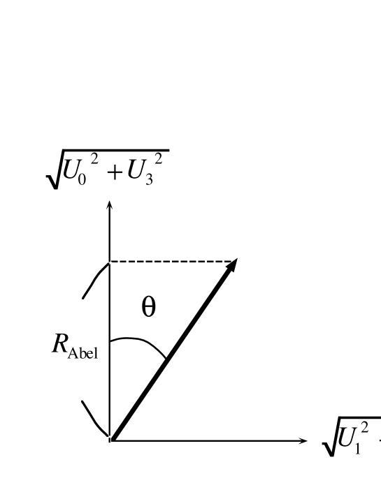
Figure 3.1: Geometrical explanation of the abelian projection rate $R_{\rm Abel}$ in terms of $U\equiv U_{0}+iU_{a}\tau_{a}$. The deviation from the vertical axis indicates the magnitude of the off-diagonal component. This description will be used in Figs 3.3 and 3.3.

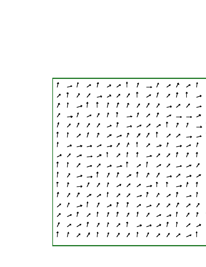
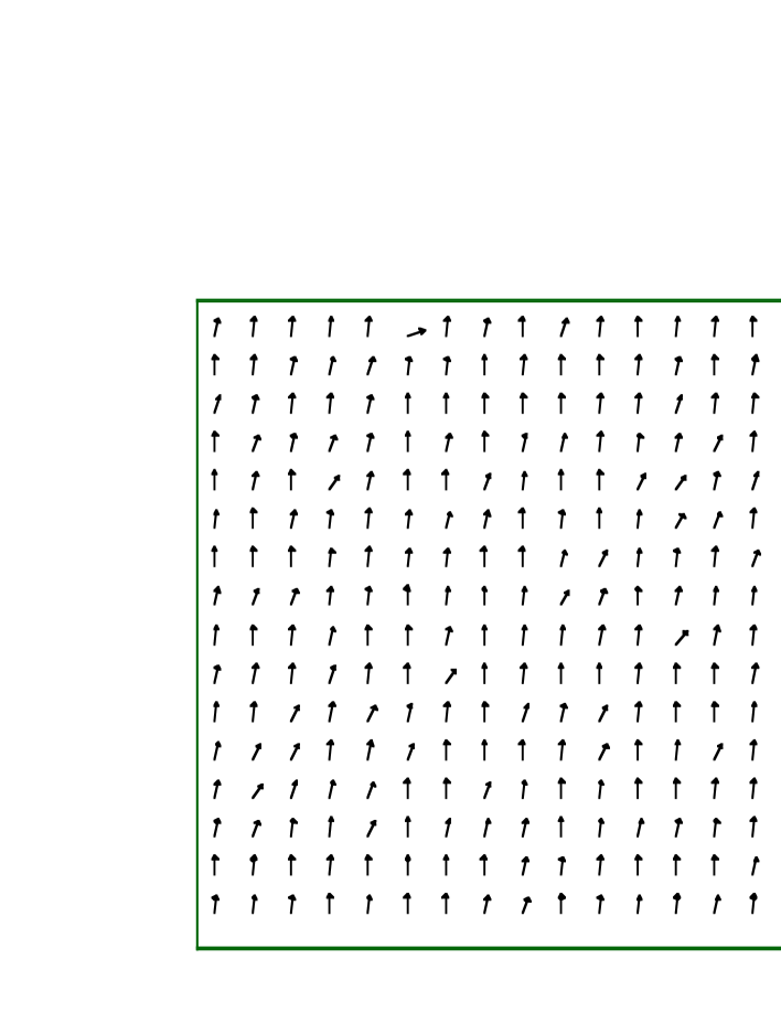
Figure 3.2: Local abelian rate $R_{\rm Abel}=\cos\theta_{\mu}(s)$ at $\beta=$2.4 on $16^{4}$ lattice without gauge fixing. The meaning of the arrow is shown in Fig.3.1.

Figure 3.3: Local abelian rate $R_{\rm Abel}=\cos\theta_{\mu}(s)$ at $\beta=$2.4 on $16^{4}$ lattice in the MA gauge. The meaning of the arrow is shown in Fig.3.1.

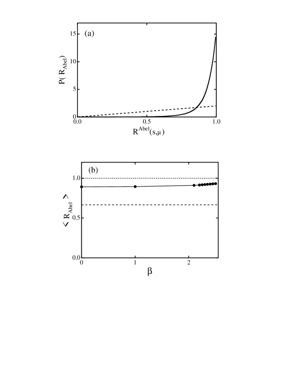
Figure 3.4: (a) The probability distribution $P(R_{\rm Abel})$ of the abelian projection rate $R_{\rm Abel}$ at $\beta=2.4$ on the $16^{4}$ lattice from 40 gauge configurations. The solid curve denotes $P(R_{\rm Abel})$ in the MA gauge, and the dashed line denotes $P(R_{\rm Abel})$ without gauge fixing. (b) The average of the abelian projection rate $\langle R_{\rm Abel}\rangle$ in the MA gauge as the function of $\beta$. For comparison, we plot also $\langle R_{\rm Abel}\rangle$ without gauge fixing.

We show in Fig.3.3 and Fig.3.3 the spatial distribution of the abelian projection rate $R_{\rm Abel}=\cos\theta$ as an arrow $(\sin\theta,\cos\theta)$. In the MA gauge, most of all SU(2) link variables become U(1)₃-like. We also show in Fig.3.4(a) the probability distribution $P(R_{\rm Abel})$ of the abelian projection rate $R_{\rm Abel}(s,\hat{\mu})$ in the MA gauge. Here, $\langle R_{\rm Abel}\rangle_{\beta=0}$ in the strong coupling limit ($\beta=0$) [50, 51] is analytically calculable as

$$\langle R_{\rm Abel}\rangle_{\beta=0} = \langle\cos\theta_{\mu}(s)\rangle_{\beta=0}=\frac{\int dU_{\mu}(s)\cos\theta_{\mu}(s)}{\int dU_{\mu}(s)}$$ (3.14)

$$= \frac{\int_{0}^{\frac{\pi}{2}}d\theta_{\mu}(s)\sin\theta_{\mu}(s)\cos^{2}\theta_{\mu}(s)}{\int_{0}^{\frac{\pi}{2}}d\theta_{\mu}(s)\sin\theta_{\mu}(s)\cos\theta_{\mu}(s)}=\frac{2}{3},$$

using Eq.(3.12). In the MA gauge, $R_{\rm Abel}$ approaches to unity as shown in Fig.3.4(a). The off-diagonal component of the SU(2) link variable is forced to be reduced. As a typical example, one obtains $\langle R_{\rm Abel}\rangle_{\rm MA}\simeq$ 0.926 on $16^{4}$ lattice with $\beta=2.4$. In Fig.3.4(b), we show the abelian projection rate $\langle R_{\rm Abel}\rangle_{\rm MA}$ as the function of $\beta$. For larger $\beta$, $\langle\cos\theta_{\mu}(s)\rangle_{\rm MA}$ becomes slightly larger. Without gauge fixing, the average $\langle R_{\rm Abel}\rangle$ is found to be about $2\over 3$ without dependence on $\beta$. In the continuum limit in the MA gauge, $U_{\mu}^{1}(s)$ and $U_{\mu}^{2}(s)$ become at most $O(a)$, and therefore $\langle R_{\rm Abel}\rangle_{\rm MA}$ approaches to unity as $\langle R_{\rm Abel}\rangle_{\rm MA}=1+O(a^{2})$ due to the trivial dominance of $U_{\mu}^{0}(s)$, which differs from abelian dominance in the physical sense. The remarkable feature of the MA gauge is the high abelian projection rate as $\langle R_{\rm Abel}\rangle_{\rm MA}\simeq 1$ in the whole region of $\beta$. In fact, we find $\langle R_{\rm Abel}\rangle_{\rm MA}\simeq 0.88$ even for the strong coupling limit $\beta=0$, where the original link variable $U_{\mu}$ is completely random. Thus, abelian dominance for the link variable $U_{\mu}$ is observed at any scale in the MA gauge.

To understand the origin of the high abelian projection rate as $\langle R_{\rm Abel}\rangle_{\rm MA}\simeq 1$, we estimate the lower bound of $\langle R_{\rm Abel}\rangle_{\rm MA}$ in the MA gauge using the statistical consideration. The MA gauge maximizes

$$R_{\rm MA}[U_{\mu}]\equiv\sum_{s,\mu}{\rm tr}\{U_{\mu}(s)\tau_{3}U^{\dagger}_{\mu}(s)\tau_{3}\}={\rm tr}(\tau_{3}\sum_{s,\mu}\hat{\phi}_{\mu}(s)),$$ (3.15)

where $\hat{\phi}_{\mu}(s)\equiv U_{\mu}(s)\tau_{3}U^{\dagger}_{\mu}(s)$ is an $su$(2) element satisfying $\hat{\phi}^{2}_{\mu}=1$. Denoting $\hat{\phi}_{\mu}(s)=\hat{\phi}^{a}_{\mu}(s)\tau^{a}$, we parameterize the 3-dimensional unit vectors $\vec{\phi}_{\mu}\equiv(\hat{\phi}_{\mu}^{1},\hat{\phi}_{\mu}^{2},\hat{\phi}_{\mu}^{3})\in S^{2}$ $(\mu=1,2,3,4)$ as $\vec{\phi}_{\mu}=(\sin 2\theta_{\mu}\cos\chi_{\mu},\sin 2\theta_{\mu}\sin\chi_{\mu},\cos 2\theta_{\mu})$ using Eqs.(3.3) and (3). The MA gauge maximizes the third component $\hat{\phi}_{\mu}^{3}$ using the gauge transformation. Under the local gauge transformation by $V(s)\equiv 1+\{V(s_{0})-1\}\delta_{ss_{0}}\in$ SU(2), $\hat{\phi}_{\mu}(s_{0})$ is transformed as the unitary transformation,

$$\hat{\phi}_{\mu}(s_{0})\rightarrow\hat{\phi}^{\prime}_{\mu}(s_{0})\equiv V(s_{0})\hat{\phi}_{\mu}(s_{0})V^{-1}(s_{0}),$$ (3.16)

which leads to a simple rotation of the unit vectors $\vec{\phi}_{\mu}$. In the MA gauge, $\displaystyle\sum_{s,\mu}$$\vec{\phi}_{\mu}$ is “polarized” along the positive third direction. On the 4-dimension lattice with $N$ sites, 4$N$ unit vectors $\vec{\phi}_{\mu}(s)$ are maximally polarized by $N$ gauge functions $V(s)$ in the MA gauge. Then, $\langle R_{\rm Abel}\rangle_{\rm MA}$ is expressed as the maximal “polarization rate” of 4$N$ unit vectors $\vec{\phi}_{\mu}$ by suitable $N$ gauge functions $V(s)$. On the average, this estimation of $\langle R_{\rm Abel}\rangle_{\rm MA}$ is approximately given by the estimation of the maximal polarization rate of 4 unit vectors $\vec{\phi}_{\mu}$ by a suitable rotation with $V\in$ SU(2). The lower bound of $\langle R_{\rm Abel}\rangle_{\rm MA}$ is obtained from the strong-coupling system with $\beta=0$, where link variables $U_{\mu}(s)$ are completely random. Accordingly, $\vec{\phi}_{\mu}$ can be regarded as random unit vectors on $S^{2}$. The maximal “polarization” of 4 unit vectors $\vec{\phi}_{\mu}$ is realized by the rotation which moves $\vec{\phi}\equiv$$\displaystyle\sum_{\mu=1}^{4}$$\vec{\phi}_{\mu}/|$$\displaystyle\sum_{\mu=1}^{4}$$\vec{\phi}_{\mu}|$ to the unit vector $\vec{\phi}^{R}\equiv(0,0,1)$ in third direction. Here, $\cos 2\theta_{\mu}^{R}$ after the rotation is identical to the inner product between $\vec{\phi}_{\mu}$ and $\vec{\phi}$, because of $\vec{\phi}\cdot\vec{\phi}_{\mu}=\vec{\phi}^{R}\cdot\vec{\phi}_{\mu}^{R}=(\hat{\phi}_{\mu}^{R})^{3}=\cos 2\theta_{\mu}^{R}$. Then, we estimate $\langle R_{\rm Abel}\rangle_{\rm MA}=\langle\cos\theta_{\mu}\rangle_{\rm MA}$ at $\beta=0$ as

$$\langle\cos\theta_{\mu}\rangle_{\rm MA}^{\beta=0}\simeq\!\{\prod_{\mu=1}^{4}\int dU_{\mu}\}\left(\frac{1}{4}\sum_{\mu=1}^{4}\cos\theta_{\mu}^{R}\right)$$ (3.17)

$$= \{\prod_{\mu=1}^{4}\frac{1}{\pi}\int_{0}^{\frac{\pi}{2}}d\theta_{\mu}\cos\theta_{\mu}\sin\theta_{\mu}\int_{-\pi}^{\pi}d\chi_{\mu}\}\left(\frac{1}{4}\sum_{\mu=1}^{4}\cos\{\frac{1}{2}\cos^{-1}(\vec{\phi}\cdot\vec{\phi}_{\mu})\}\right).$$

Using this estimation (3.17), we obtain $\langle R_{\rm Abel}\rangle_{\rm MA}\simeq$ 0.844, which is close to the lattice result $\langle R_{\rm Abel}\rangle\simeq$ 0.88 in the strong coupling limit ($\beta=0$). Such a high abelian rate $\langle R_{\rm Abel}\rangle_{\rm MA}$ in the MA gauge would provide a microscopic basis of abelian dominance for the infrared physics.

3.2 Abelian Dominance for Confinement Force in the MA Gauge

In this section, we study the origin of abelian dominance on the string tension as the confinement force in a semi-analytical manner, considering the relation with microscopic abelian dominance on the link variable [27, 51].

In the MA gauge, the diagonal element $\cos\theta_{\mu}(s)$ in $M_{\mu}(s)$ is maximized by the gauge transformation as large as possible. For instance, the abelian projection rate is almost unity as $R_{\rm Abel}=\langle\cos\theta_{\mu}(s)\rangle_{\rm MA}\simeq 0.93$ at $\beta=2.4$. Then, the off-diagonal element $e^{i\chi_{\mu}(s)}\sin\theta_{\mu}(s)$ is forced to take a small value in the MA gauge due to the factor $\sin\theta_{\mu}(s)$, and therefore the approximate treatment on the off-diagonal element would be allowed in the MA gauge. Moreover, the angle variable $\chi_{\mu}(s)$ is not constrained by the MA gauge-fixing condition at all, and tends to take a random value besides the residual ${\rm U(1)}_{3}$ gauge degrees of freedom. Hence, $\chi_{\mu}(s)$ can be regarded as a random angle variable on the treatment of $M_{\mu}(s)$ in the MA gauge in a good approximation.

Let us consider the Wilson loop $\displaystyle\langle W_{C}[U_{\mu}(s)]\rangle\equiv\langle{\rm tr}\prod_{C}U_{\mu}(s)\rangle=\langle{\rm tr}\prod_{C}\{M_{\mu}(s)u_{\mu}(s)\}\rangle$ in the MA gauge. In calculating $\langle W_{C}[U_{\mu}(s)]\rangle$, the expectation value of $e^{i\chi_{\mu}(s)}$ in $M_{\mu}(s)$ vanishes as

$$\langle e^{i\chi_{\mu}(s)}\rangle\simeq\int_{0}^{2\pi}d\chi_{\mu}(s)\exp\{i\chi_{\mu}(s)\}=0,$$ (3.18)

when $\chi_{\mu}(s)$ behaves as a random angle variable. Then, within the random-variable approximation for $\chi_{\mu}(s)$, the off-diagonal factor $M_{\mu}(s)$ appearing in $\langle W_{C}[U_{\mu}(s)]\rangle$ is simply reduced as a $c$-number factor, $M_{\mu}(s)\rightarrow\cos\theta_{\mu}(s)\ {\bf 1},$ and therefore the SU(2) link variable $U_{\mu}(s)$ in the Wilson loop $\langle W_{C}[U_{\mu}(s)]\rangle$ is simplified as a diagonal matrix,

$$U_{\mu}(s)\equiv M_{\mu}(s)u_{\mu}(s)\rightarrow\cos\theta_{\mu}(s)u_{\mu}(s).$$ (3.19)

Then, for the $I\times J$ rectangular $C$, the Wilson loop $W_{C}[U_{\mu}(s)]$ in the MA gauge is approximated as

$$\langle W_{C}[U_{\mu}(s)]\rangle \equiv \langle{\rm tr}\prod_{i=1}^{L}U_{\mu_{i}}(s_{i})\rangle\simeq\langle\prod_{i=1}^{L}\cos\theta_{\mu_{i}}(s_{i})\cdot{\rm tr}\prod_{j=1}^{L}u_{\mu_{j}}(s_{j})\rangle_{\rm MA}$$ (3.20)

$$\simeq \langle\exp\{\sum_{i=1}^{L}\ln(\cos\theta_{\mu_{i}}(s_{i}))\}\rangle_{\rm MA}\ \langle W_{C}[u_{\mu}(s)]\rangle_{\rm MA}$$ (3.21)

$$\simeq \exp\{L\langle\ln(\cos\theta_{\mu}(s))\rangle_{\rm MA}\}\ \langle W_{C}[u_{\mu}(s)]\rangle_{\rm MA},$$ (3.22)

where $L\equiv 2(I+J)$ denotes the perimeter length and $\displaystyle W_{C}[u_{\mu}(s)]\equiv{\rm tr}\prod_{i=1}^{L}u_{\mu_{i}}(s_{i})$ the abelian Wilson loop. Here, we have replaced $\displaystyle\sum_{i=1}^{L}\ln\{\cos(\theta_{\mu_{i}}(s_{i})\}$ by its average $L\langle\ln\{\cos\theta_{\mu}(s)\}\rangle_{\rm MA}$ in a statistical sense, and such a statistical treatment becomes more accurate for larger $I,J$ and becomes exact for infinite $I,J$.

In this way, we derive a simple estimation as

$$W_{C}^{\rm off}\equiv\langle W_{C}[U_{\mu}(s)]\rangle/\langle W_{C}[u_{\mu}(s)]\rangle_{\rm MA}\simeq\exp\{L\langle\ln(\cos\theta_{\mu}(s))\rangle_{\rm MA}\}$$ (3.23)

for the contribution of the off-diagonal gluon element to the Wilson loop. From this analysis, the contribution of off-diagonal gluons to the Wilson loop is expected to obey the perimeter law in the MA gauge for large loops, where the statistical treatment would be accurate.

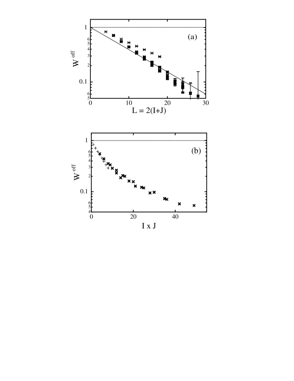
Figure 3.5: The off-diagonal gluon contribution on the Wilson loop, $W^{\rm off}\equiv\frac{\langle W_{C}[U_{\mu}(s)]\rangle}{\langle W_{C}[u_{\mu}(s)]\rangle}$, as the function of the perimeter length $L\equiv 2(I+J)$ in the MA gauge on $16^{4}$ lattice with $\beta=2.4$. The thick line denotes the theoretical estimation in Eq.(3.23) with the microscopic input $\langle\ln\{\cos\theta_{\mu}(s)\}\rangle_{\rm MA}\simeq-0.082$ at $\beta=2.4$. The data of the Wilson loop with $I=1$ or $J=1$ are distinguished by the thin cross.

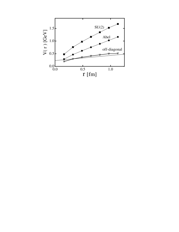
Figure 3.6: The inter-quark potential $V(r)$ as the function of the inter-quark distance $r$. The lattice data are obtained from the Wilson loop in the MA gauge on $16^{4}$ lattice with $\beta=2.4$ and $T=7$. The square, the circle and the rhombus denote the full SU(2), the abelian and the off-diagonal contribution of the static potential, respectively. The thin line denotes the theoretical estimation in Eq.(3.27). Here, the lattice spacing $a$ is determined so as to produce $\sigma=0.89$ GeV/fm. Due to the artificial finite-size effect of the Wilson loop, the off-diagonal contribution $V^{\rm off}$ gets a slight linear part.

Now, we study the behavior of the off-diagonal contribution
$W_{C}^{\rm off}\equiv\langle W_{C}[U_{\mu}(s)]\rangle/\langle W_{C}[u_{\mu}(s)]\rangle_{\rm MA}$ in the MA gauge using the lattice QCD, considering the theoretical estimation Eq.(3.23). As shown in Fig.3.5, we find that $W_{C}^{\rm off}$ seems to obey the perimeter law for the Wilson loop with $I,J\geq 2$ in the MA gauge in the lattice QCD simulation with $\beta=2.4$ and $16^{4}$. We find also that the behavior on $W_{C}^{\rm off}$ as the function of $L$ is well reproduced by the above analytical estimation with microscopic information on the diagonal factor $\cos\theta_{\mu}(s)$ as $\langle\ln\{\cos\theta_{\mu}(s)\}\rangle_{\rm MA}\simeq-0.082$ for $\beta=2.4$. Thus, the off-diagonal contribution $W_{C}^{\rm off}$ to the Wilson loop obeys the perimeter law in the MA gauge, and therefore the abelian Wilson loop $\langle W_{C}[u_{\mu}(s)]\rangle_{\rm MA}$ should obey the area law as well as the SU(2) Wilson loop $W_{C}[U_{\mu}(s)]$. From Eq.(3.23), the off-diagonal contribution to the string tension vanishes as

$$\Delta\sigma \equiv \sigma_{\rm SU(2)}-\sigma_{\rm Abel}$$

$$\equiv -\lim_{R,T\rightarrow\infty}{1\over RT}\ln\langle W_{R\times T}[U_{\mu}(s)]\rangle+\lim_{R,T\rightarrow\infty}{1\over RT}\ln\langle W_{R\times T}[u_{\mu}(s)]\rangle_{\rm MA}$$

$$\simeq -2\langle\ln\{\cos\theta_{\mu}(s)\}\rangle_{\rm MA}\lim_{R,T\rightarrow\infty}{R+T\over RT}=0.$$ (3.25)

Thus, abelian dominance for the string tension, $\sigma_{\rm SU(2)}=\sigma_{\rm Abel}$, can be proved in the MA gauge by replacing the off-diagonal angle variable $\chi_{\mu}(s)$ as a random variable.

The analytical relation in Eq.(3.23) indicates also that the finite size effect on $R$ and $T$ in the Wilson loop leads to the deviation between the SU(2) string tension $\sigma_{\rm SU(2)}$ and the abelian string tension $\sigma_{\rm Abel}$ as $\sigma_{\rm SU(2)}>\sigma_{\rm Abel}$ in the actual lattice QCD simulations. Here, we consider this deviation $\Delta\sigma\equiv\sigma_{\rm SU(2)}-\sigma_{\rm Abel}$ in some detail. Similar to the SU(2) inter-quark potential $V_{\rm SU(2)}(r)$ from $\langle\,W_{\rm SU(2)}\,\rangle\equiv\langle\,W[U_{\mu}(s)]\,\rangle$, we define the abelian inter-quark potential $V_{\rm Abel}(r)$ and the off-diagonal contribution $V_{\rm off}(r)$ of the potential from $\langle\,W_{\rm Abel}\,\rangle\equiv\langle\,W[u_{\mu}(s)]\,\rangle$ and $W_{\rm off}$, respectively,

$$V_{\rm SU(2)}(r) \equiv -\frac{1}{Ta}{\rm ln}\,\langle\,W_{\rm SU(2)}({R\times T})\,\rangle,$$

$$V_{\rm Abel}(r) \equiv -\frac{1}{Ta}{\rm ln}\,\langle\,W_{\rm Abel}({R\times T})\,\rangle,$$

$$V_{\rm off}(r) \equiv -\frac{1}{Ta}{\rm ln}\,W_{\rm off}({R\times T})=-\frac{1}{Ta}{\rm ln}\,\frac{\langle\,W_{\rm SU(2)}({R\times T})\,\rangle}{\langle\,W_{\rm Abel}({R\times T})\,\rangle}$$ (3.26)

$$= V_{\rm SU(2)}(r)-V_{\rm Abel}(r),$$

where $r\equiv Ra$ denotes the inter-quark distance in the physical unit. We show in Fig.3.6 $V_{\rm SU(2)}(r)$, $V_{\rm Abel}(r)$ and $V_{\rm off}(r)$ extracted from the Wilson loop with $T=7$ in the lattice QCD simulation with $\beta=2.4$ and $16^{4}$. As shown in Fig.3.6, the lattice result for $V_{\rm off}(r)$ seems to be reproduced by the theoretical estimation obtained from Eq.(3.23),

$$V_{\rm off}(r)=V_{\rm SU(2)}(r)-V_{\rm Abel}(r)\simeq-\frac{2(R+T)}{Ta}\langle\ln(\cos\theta_{\mu}(s))\rangle_{\rm MA}$$ (3.27)

using the microscopic information of $\langle\ln(\cos\theta_{\mu}(s))\rangle_{\rm MA}=-0.082$ at $\beta=2.4$. From the slope of $V_{\rm off}(r)$ in Eq.(3.27), we can estimate $\Delta\sigma\equiv\sigma_{\rm SU(2)}-\sigma_{\rm Abel}$ in the physical unit as

$$\Delta\sigma\equiv\sigma_{\rm SU(2)}-\sigma_{\rm Abel} \simeq -2\langle\,\ln\,(\,\cos\theta_{\mu}(s)\,)\,\rangle_{\rm MA}\,\frac{1}{Ta^{2}}$$ (3.28)

$$= -\langle\ln(1-\sin^{2}\theta_{\mu}(s))\rangle_{\rm MA}\frac{1}{Ta^{2}}.$$

In the MA gauge, $\sin^{2}\theta_{\mu}(s)$ takes a small value and can be treated in a perturbation manner so that one finds

$$\Delta\sigma\simeq\langle\sin^{2}\theta_{\mu}(s)\rangle_{\rm MA}\frac{1}{Ta^{2}}=\langle(U^{1}_{\mu}(s))^{2}+(U^{2}_{\mu 2}(s))^{2}\rangle_{\rm MA}\frac{1}{Ta^{2}}.$$ (3.29)

Near the continuum limit $a\simeq 0$, we find $U_{\mu}^{a}\simeq aeA_{\mu}^{a}/2$ ($a$=1,2,3) from $U_{\mu}=e^{iaeA_{\mu}^{a}{\tau^{a}}/{2}}$, and then we derive the relation between $\Delta\sigma$ and the off-diagonal gluon in the MA gauge as

$$\Delta\sigma\simeq\frac{1}{4T}\langle(eA_{\mu}^{1})^{2}+(eA_{\mu}^{2})^{2}\rangle_{\rm MA}=\frac{a}{4t}\langle(eA_{\mu}^{1})^{2}+(eA_{\mu}^{2})^{2}\rangle_{\rm MA},$$ (3.30)

where $t\equiv Ta$ is the temporal length of the Wilson loop in the physical unit. In Eq.(3.30), $\langle(eA_{\mu}^{1})^{2}+(eA_{\mu}^{2})^{2}\rangle_{\rm MA}$ is the off-diagonal gluon-field fluctuation, and is strongly suppressed in the MA gauge by its definition. It would be interesting to note that microscopic abelian dominance or the suppression of off-diagonal gluons in the MA gauge is directly connected to reduction of the deviation $\Delta\sigma$ in Eq.(3.30). Since $\langle(eA_{\mu}^{1})^{2}+(eA_{\mu}^{2})^{2}\rangle_{\rm MA}$ is a local continuum quantity, it is to be independent on both $a$ and $t$. Hence, the deviation $\Delta\sigma$ between the SU(2) string tension $\sigma_{\rm SU(2)}$ and the abelian string tension $\sigma_{\rm Abel}$ can be removed by taking the large Wilson loop as $t\rightarrow\infty$ or the small mesh as $a\rightarrow 0$ with fixed $t$.

3.3 Gluon Field in the MA Gauge with the U(1)₃ Landau Gauge

In the MA gauge, the linear confinement potential can be almost reproduced only by the abelian degrees of freedom, which is called as abelian dominance on the string tension. In this section, we study the probability distribution of the gauge field such as the abelian gauge field, the abelian field strength, the off-diagonal gluon in the MA gauge.

From the abelian angle variable $\theta^{3}_{\mu}(s)$, the abelian field strength ${\bar{\theta}_{\mu\nu}}(s)$ is defined as

$${\bar{\theta}_{\mu\nu}}(s)\equiv{\rm mod}_{2\pi}(\partial\wedge\theta^{3})_{\mu\nu}(s)\in(-\pi,\pi],$$ (3.31)

where $(\partial\wedge\theta^{3})_{\mu\nu}(s)$ is expressed as

$$(\partial\wedge\theta^{\rm 3})_{\mu\nu}(s)\equiv\theta_{\mu\nu}(s)\equiv\theta^{\rm 3}_{\mu}(s)+\theta^{\rm 3}_{\nu}(s+\hat{\mu})-\theta^{\rm 3}_{\mu}(s+\hat{\nu})-\theta^{\rm 3}_{\nu}(s).$$ (3.32)

The abelian field strength ${\bar{\theta}_{\mu\nu}}(s)$ is related to the abelian plaquette as

$$\Box^{\rm Abel}_{\mu\nu}(s)\equiv u_{\mu}(s)u_{\nu}(s+\hat{\mu})u^{\dagger}_{\mu}(s+\hat{\nu})u_{\nu}^{\dagger}(s)=e^{i\bar{\theta}_{\mu\nu}(s)}.$$ (3.33)

In terms of the U(1)₃ gauge symmetry remaining in the abelian gauge, the abelian field strength ${\bar{\theta}_{\mu\nu}}(s)$ is a U(1)₃ gauge-invariant quantity because of the gauge invariance of the abelian plaquette, while both $\theta^{3}_{\mu}(s)$ and $(\partial\wedge\theta^{3})_{\mu\nu}(s)$ are U(1)₃ gauge variant.

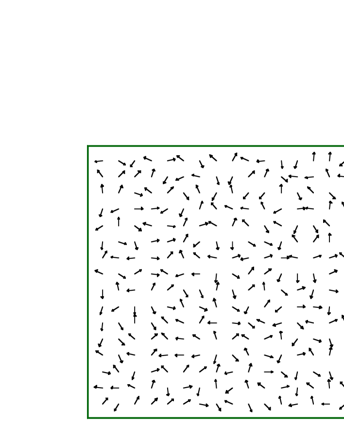
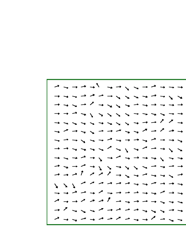
Figure 3.7: The abelian angle variable $\theta_{\mu}^{3}(s)$ without U(1)₃ Landau gauge fixing in the MA gauge at $\beta=2.4$.

Figure 3.8: The abelian angle variable $\theta_{\mu}^{3}(s)$ in the MA gauge with U(1)₃ Landau gauge fixing.

To investigate the features of U(1)₃ gauge-variant quantities like the abelian angle variable $\theta^{3}_{\mu}(s)$, it is necessary to fix the residual U(1)₃ gauge degrees of freedom in addition to the abelian gauge fixing. In this paper, we introduce U(1)₃ lattice Landau gauge [53], where the gluon field is mostly continuous under the constraint of the MA gauge condition, and the lattice field can be compared with continuum field variable more directly.

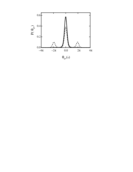
Figure 3.9: The probability distribution $P(\theta_{\mu}^{3})$ of the abelian angle variable $\theta^{3}_{\mu}(s)\in(-\pi,\pi]$ in the MA gauge on $16^{4}$ lattice with $\beta=2.4$. The solid curve denotes $P(\theta_{\mu}^{3})$ in the U(1)₃ Landau gauge fixing after the MA gauge fixing, and the dashed line denotes $P(\theta^{3}_{\mu})$ without the U(1)₃ gauge fixing. Without the U(1)₃ gauge fixing, the angle variable $\theta^{3}_{\mu}(s)$ is randomly distributed, while $\theta^{3}_{\mu}(s)$ has a Gaussian-type peak around $\theta^{3}_{\mu}(s)=0$ in the U(1)₃ Landau gauge.

Figure 3.10: The probability distributions $P(\theta_{\mu\nu})$ of the two form $\theta_{\mu\nu}\equiv(\partial\wedge\theta)_{\mu\nu}(s)$ in the MA gauge with and without U(1)₃-Landau gauge fixing, which are denoted by the solid and dashed curves, respectively. In the U(1)₃-Landau gauge, $P(\theta_{\mu\nu})$ has single peak around $\theta_{\mu\nu}=0$.

The U(1)₃ lattice Landau gauge is defined by maximizing

$$R_{L}[U_{\mu}]\equiv\displaystyle\sum_{s,\mu}{\rm Re}\,\,u_{\mu}(s)$$ (3.34)

using the residual U(1)₃ gauge transformation. In the U(1)₃ Landau gauge, the abelian angle variable $\theta^{3}_{\mu}(s)$ is suppressed as small as possible. In the continuum limit $a\rightarrow 0$, the abelian gauge field $A_{\mu}^{3}(x)$ satisfies the ordinary Lorentz-gauge condition as in QED, $\partial_{\mu}A_{\mu}^{3}=0$.

We show in Figs 3.8 and 3.8 the configuration of the abelian angle variable $\theta^{3}_{\mu}(s)$ before and after the U(1)₃ Landau gauge fixing in the MA gauge at $\beta=2.4$. The magnitude of the angle variable is found to become small and continuous in the U(1)₃ Landau gauge. We show also in Fig.3.10 the probability distribution $P(\theta_{\mu}^{3})$ of the abelian angle variable $\theta^{3}_{\mu}(s)\in(-\pi,\pi]$ in the MA gauge with and without U(1)₃ Landau gauge fixing. We find that the whole shape of the distribution seems Gaussian-type peak around $\theta_{\mu}^{3}=0$ in the U(1)₃ Landau gauge, while $\theta^{3}_{\mu}(s)$ is not settled without the U(1)₃ gauge fixing.

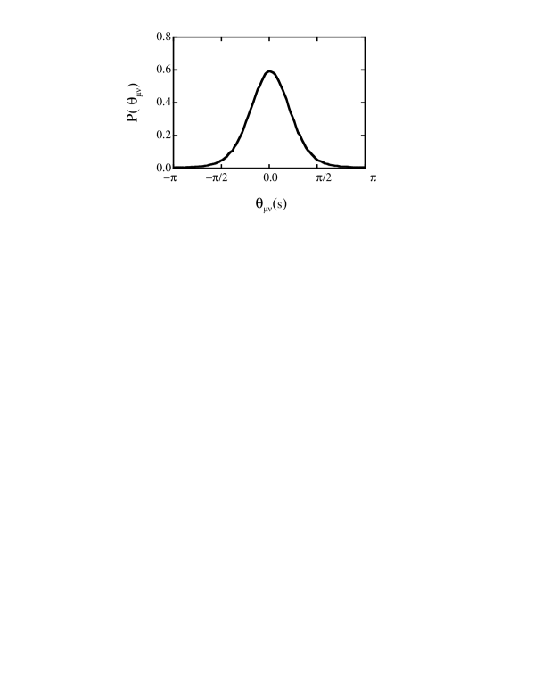
Figure 3.11: The probability distribution $P(\bar{\theta}_{\mu\nu})$ of the abelian field strength $\bar{\theta}_{\mu\nu}(s)$, which is U(1)₃ gauge invariant.

Figure 3.12: The probability distributions $P(\chi_{\mu})$ (solid line) and $P(\theta^{3}_{\mu})$ (dash-dotted curve) in the MA gauge with the U$(1)_{3}$ Landau gauge at $\beta=2.4$ on the $16^{4}$ lattice from 40 gauge configurations.

We show in Fig.3.10 the probability distribution $P(\theta_{\mu\nu})$ of the two form $\theta_{\mu\nu}(s)\equiv(\partial\wedge\theta^{\rm 3})_{\mu\nu}(s)$ of the abelian field $\theta^{3}_{\mu}(s)$. Without the gauge fixing, there appear three peaks around $\theta_{\mu\nu}(s)=$ $-2\pi$, $0$, $2\pi$. In the MA gauge, because of $U_{\mu}\simeq u_{\mu}$, not only the SU(2) action $\displaystyle\hat{S}\equiv S/\beta=\sum_{s,\mu>\nu}[1-\frac{1}{2}{\rm tr}\Box_{\mu\nu}(s)]$ but also the abelian action $\displaystyle\hat{S}^{\rm Abel}\equiv\sum_{s,\mu>\nu}[1-\frac{1}{2}{\rm tr}\Box^{\rm Abel}_{\mu\nu}(s)]$ is suppressed by the action factor $e^{-\beta\hat{S}}$ in the partition functional. Since the abelian action is written by $\displaystyle\sum_{s,\mu>\nu}[1-\cos(\theta_{\mu\nu})]$, $P(\theta_{\mu\nu})$ has peaks around $\cos(\theta_{\mu\nu})=1$. As shown in Fig.3.10, most of $\theta_{\mu\nu}(s)$ distribute around $\theta_{\mu\nu}(s)=0$ in the U(1)₃ Landau gauge, because the abelian gauge field is mostly continuous in the U(1)₃ Landau gauge. On the other hand, the probability distribution $P(\bar{\theta}_{\mu\nu})$ of the abelian field strength $\bar{\theta}_{\mu\nu}\in(-\pi,\pi]$ is U(1)₃ gauge invariant. The whole shape of $P(\bar{\theta}_{\mu\nu})$ is Gaussian-type, as shown in Fig.3.11.

Finally in this section, we investigate the off-diagonal phase variable $\chi_{\mu}(s)$ in Eq.(3). We show in Fig.3.12(a) the probability distributions $P(\chi_{\mu})$ and $P(\theta^{3}_{\mu})$ at $\beta=2.4$ in the MA gauge with U(1)₃ Landau gauge. Unlike $P(\theta^{3}_{\mu})$, $P(\chi_{\mu})$ is flat distribution without any structure. This property on the off-diagonal element would lead to the validity of the random-variable approximation for $\chi_{\mu}(s)$, which has been used for estimation of the Wilson loop in Eq.(3.22).

3.4 Randomness of Off-diagonal Gluon Phase and Abelian Dominance

In this section, we reconsider the origin of abelian dominance in the MA gauge in terms of the properties of the off-diagonal element

$$c_{\mu}(s)\equiv e^{i\chi_{\mu}(s)}\sin\theta_{\mu}(s)$$ (3.35)

in $M_{\mu}(s)$ in the link variable $U_{\mu}(s)$, considering the validity of the random-variable approximation for $\chi_{\mu}(s)$ in the MA gauge with U(1)₃ Landau gauge [27]. In this treatment, the contribution of the off-diagonal element in the link variable $U_{\mu}(s)$ is completely dropped off, and its effect indirectly remains as the appearance of the $c$-number factor $\cos\theta_{\mu}(s)$ in the link variable. Such a reduction of the contribution of the off-diagonal elements is brought by the two relevant features on the two local variables, $\theta_{\mu}(s)$ and $\chi_{\mu}(s)$, in the MA gauge. One is microscopic abelian dominance as $\langle\cos\theta_{\mu}(s)\rangle_{\rm MA}\simeq 1$ in the MA gauge, and the other is the randomness of the off-diagonal phase variable $\chi_{\mu}(s)$.

1. In the MA gauge, microscopic abelian dominance holds as $\langle\cos\theta_{\mu}(s)\rangle_{\rm MA}$ $\simeq 1$, and the absolute value of the off-diagonal element $|c_{\mu}(s)|=|\sin\theta_{\mu}(s)|$ is strongly reduced. Such a tendency becomes more significant as $\beta$ increases.

2. The off-diagonal angle variable $\chi_{\mu}(s)$ is not constrained by the MA gauge-fixing condition at all, and tends to be a random variable. In fact, $\chi_{\mu}(s)$ is affected only by the QCD action factor $e^{-\beta\hat{S}_{\rm QCD}}$ in the QCD generating functional, but the effect of the action to $\chi_{\mu}(s)$ is quite weaken due to the small factor $\sin\theta_{\mu}(s)$ in the MA gauge. The randomness of $\chi_{\mu}(s)$ tends to vanish the contribution of the off-diagonal elements.

Here, the randomness of the off-diagonal angle-variable $\chi_{\mu}(s)$ is closely related to microscopic abelian dominance. In fact, the randomness of $\chi_{\mu}(s)$ is controlled only by the action factor $e^{-\beta\hat{S}_{\rm QCD}}$ in the QCD generating functional, however the effect of the action to $\chi_{\mu}(s)$ is quite weaken due to the small factor $\sin\theta_{\mu}(s)$ in the MA gauge, because $\chi_{\mu}(s)$ always accompanies $\sin\theta_{\mu}(s)$ in the link variable $U_{\mu}(s)$. Near the strong-coupling limit $\beta\simeq 0$, the action factor $e^{-\beta\hat{S}_{\rm QCD}}$ brings almost no constraint on $\chi_{\mu}(s)$ in the MA gauge. The independence of $\chi_{\mu}(s)$ from the action factor is enhanced by the small factor $\sin\theta_{\mu}(s)$ accompanying $\chi_{\mu}(s)$. Hence, $\chi_{\mu}(s)$ behaves as a random angle-variable almost exactly, and the contribution of the off-diagonal element is expected to disappear in the strong-coupling region. As $\beta$ increases, the action factor $e^{-\beta\hat{S}_{\rm QCD}}$ becomes relevant and will reduce the randomness of $\chi_{\mu}(s)$ to some extent. Near the continuum limit $\beta\rightarrow\infty$, however, the factor $\sin\theta_{\mu}(s)$ tends to approach 0 in the MA gauge as shown in Fig.3.4(b), and hence such a constraint on $\chi_{\mu}(s)$ from the action is largely reduced, and the strong randomness of $\chi_{\mu}(s)$ is expected to hold there. Moreover, the reduction of the absolute value $|c_{\mu}(s)|=|\sin\theta_{\mu}(s)|$ itself further reduces the contribution of the off-diagonal element $|c_{\mu}(s)|$ in the MA gauge.

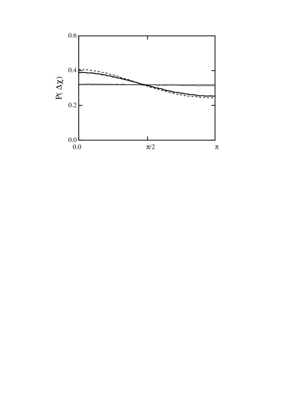
Figure 3.13: The probability distribution $P(\Delta\chi)$ of the correlation $\Delta\chi\equiv{\rm mod}_{\pi}(|\chi_{\mu}(s)-\chi_{\mu}(s+\hat{\nu})|)$ in the same gauge at $\beta$ = 0 (thin line), 1.0 (dotted curve), 2.4 (solid curve), 3.0 (dashed curve).

Now, we examine the randomness of $\chi_{\mu}(s)$ using the lattice QCD simulation. We calculate the correlation between $\chi_{\mu}(s)$ and $\chi_{\mu}(s+\hat{\nu})$ in the MA gauge with the U(1)₃-Landau gauge. If $\chi_{\mu}(s)$ is an exact random angle variable, no correlation is observed between $\chi_{\mu}(s)$ and $\chi_{\mu}(s+\hat{\nu})$. We show in Fig.3.13 the probability distribution $P(\Delta\chi)$ of the correlation

$$\Delta\chi(s)\equiv d(\chi_{\mu}(s),\chi_{\mu}(s+\hat{\nu}))\equiv{\rm mod}_{\pi}|\chi_{\mu}(s)-\chi_{\mu}(s+\hat{\nu})|\in[0,\pi],$$ (3.36)

which is the difference between two neighboring angle variables, at $\beta$=0, 1.0, 2.4, 3.0. In the strong-coupling limit $\beta=0$, $\chi_{\mu}(s)$ is a completely random variable, and there is no correlation between neighboring $\chi_{\mu}$. In the strong-coupling region as $\beta\leq 1.0$, almost no correlation is observed between neighboring $\chi_{\mu}$, which suggests the strong randomness of $\chi_{\mu}(s)$. As a remarkable feature, the correlation between neighboring $\chi_{\mu}$ seems weak even in the weak-coupling region as $\beta\geq 2.4$, where the action factor $e^{-\beta\hat{S}_{\rm QCD}}$ becomes dominant and remaining variables $\theta_{\mu}^{3}(s)$ and $\theta_{\mu}(s)$ behave as continuous variables with small difference between their neighbors as $\Delta\theta_{\mu}^{3}\simeq 0$ and $\Delta\theta_{\mu}\simeq 0$. Such a weak correlation of neighboring $\chi_{\mu}$ would be originated from the reduction of the accompanying factor $\sin\theta_{\mu}(s)$ in the MA gauge. Moreover, in the weak-coupling region, the smallness of $\sin\theta_{\mu}(s)$ makes $c_{\mu}(s)$ more irrelevant in the MA gauge, which permits some approximation on $\chi_{\mu}(s)$. Thus, the random-variable approximation for $\chi_{\mu}(s)$ would provide a good approximation in the whole region of $\beta$ in the MA gauge. To conclude, the origin of abelian dominance for confinement in the MA gauge is stemming from the strong randomness of the off-diagonal angle variable $\chi_{\mu}(s)$ and the strong reduction of the off-diagonal amplitude $|\sin\theta_{\mu}(s)|$ as the result of the MA gauge fixing.

3.5 Comparison with SU(2) Landau Gauge

In this section, we study the feature of the MA gauge in terms of the concentration of the gluon field fluctuation into the U(1)₃ sector by comparison with the SU(2) Landau gauge [53]. In the MA gauge, off-diagonal gluon components are forced to be small by the gauge transformation. Instead, the gluon field fluctuation is maximally concentrated into the abelian sector, and monopoles appear in the abelian sector as the result of the large fluctuation of the abelian field component. For the qualitative argument on the share of the gluon fluctuation into each component, we measure $\langle U_{\mu}^{a}(s)\rangle$ ($a$ =1,2,3) and

$$R_{\rm diag}(s) \equiv \frac{U^{3}_{\mu}(s)^{2}}{U^{1}_{\mu}(s)^{2}+U^{2}_{\mu}(s)^{2}+U^{3}_{\mu}(s)^{2}}.$$ (3.37)

In the MA gauge with the U(1)₃ Landau gauge, we find a strong concentration of the gluon field fluctuation into the abelian sector as $\langle U_{\mu}^{1}(s)\rangle=\langle U_{\mu}^{2}(s)\rangle\ll\langle U_{\mu}^{3}(s)\rangle$ and $R_{\rm diag}\gg\frac{1}{3};$ as a typical example, we find at $\beta=2.4$ $\langle U_{\mu}^{1}(s)\rangle=\langle U_{\mu}^{2}(s)\rangle\simeq 0.067$, $\langle U_{\mu}^{3}(s)\rangle\simeq 0.43$ and $R_{\rm diag}\simeq 0.68$.

For comparison, we consider the SU(2) lattice Landau gauge [53] defined by maximizing

$$R_{L}[U_{\mu}]\equiv\sum_{s,\mu}{\rm tr}U_{\mu}(s)=2\sum_{s,\mu}U^{0}_{\mu}(s),$$ (3.38)

where all the lattice gluon components fields become mostly continuous owing to the suppression of their fluctuation around $U_{\mu}(s)=1$. In the continuum limit, this gauge fixing condition coincides the ordinary SU(2) Landau gauge condition $\partial_{\mu}A_{\mu}=0$. In the lattice SU(2) Landau gauge, one finds $R_{\rm diag}=\frac{1}{3}$ and $\langle U_{\mu}^{1}(s)\rangle=\langle U_{\mu}^{2}(s)\rangle=\langle U_{\mu}^{3}(s)\rangle\ll 1$, for instance $\langle U_{\mu}^{a}(s)\rangle=$ 0.076 at $\beta=2.4$, so that all the gluon components are forced to be small equally.

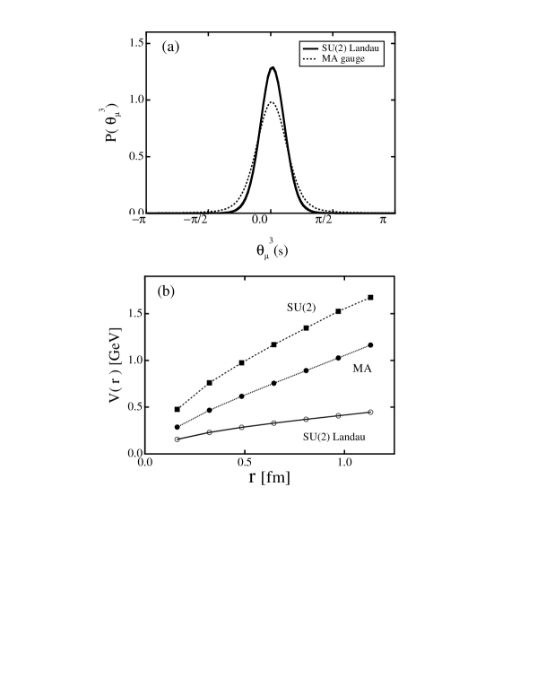
Figure 3.14: Comparison between the MA gauge and the SU(2) Landau gauge with global SU(2)/(U(1) $\times$ Weyl) fixed. (a) The probability distribution $P(\theta^{3}_{\mu})$ of the lattice angle variable $\theta^{3}_{\mu}(s)$ in the SU(2) Landau gauge (solid curve) and the MA gauge (dotted curve ) with $\beta=2.4$ on $16^{4}$ lattice. The large fluctuation on the link variable $\theta^{3}_{\mu}(s)$ disappears in the SU(2) Landau gauge. The abelian part of the interquark potential $V(r)$ as the function of interquark distance $r$ in the SU(2) Landau gauge and in the MA gauge on $16^{4}$ lattice with $\beta=2.4$. For comparison, the full SU(2) result is added.

In the SU(2) Landau gauge, the local symmetry of SU(2) is fixed, and only the global SU(2) symmetry remains, because $\displaystyle R_{L}[U_{\mu}]\equiv\sum_{s,\mu}{\rm tr}U_{\mu}(s)$ is invariant by any global gauge transformation. In order to compare with the MA gauge, we fix SU(2)/(U(1)₃ $\times$ Weyl) in this global SU(2) symmetry by the additional condition so as to maximize $\displaystyle R_{\rm MA}[U_{\mu}]=\sum_{s,\mu}{\rm tr}(U_{\mu}(s)\tau_{3}U_{\mu}^{\dagger}(s)\tau_{3})$ by the remaining global SU(2) gauge transformation. Here, the SU(2) Landau gauge with SU(2)_global/(U(1)${}_{3\rm global}\times$ Weyl) fixing is regarded as a kind of the abelian gauge. Then, we can extract the abelian variable $\theta_{\mu}^{3}(s)$ even for this SU(2) Landau gauge. Figure 3.14(a) shows the probability distribution $P(\theta_{\mu}^{3})$ of the abelian angle variable $\theta_{\mu}^{3}(s)$ in the SU(2) Landau gauge and in the MA gauge at $\beta=2.4$. We show also in Fig.3.14(b) the interquark potential in the abelian sector evaluated from the abelian Wilson loop in these gauges. Although the global shape of the distribution $P(\theta_{\mu}^{3})$ in the SU(2) Landau gauge is similar to that in the MA gauge except for the reduction of the large fluctuation apart from $\theta_{\mu}^{3}(s)=0$, the abelian string tension in the SU(2) Landau gauge is much smaller than that in the MA gauge [30]. Therefore, the large fluctuation ingredient is expected to be responsible for the confinement property.

To summarize, in the MA gauge, the field fluctuation is maximally concentrated into the abelian sector, and hence large fluctuation ingredient appears and the confinement property is almost reproduced only by the abelian variable. Another clear difference between the MA gauge and the SU(2) Landau gauge observed on lattice is the density of monopoles appearing in the abelian sector. Indeed, the SU(2) Landau gauge includes scarcely monopoles in the abelian sector in comparison with the MA gauge, for instance, the ratio on the monopole density is less than 1/10 at $\beta=2.4$. This result seems natural because the SU(2) Landau gauge fixing provides a mostly continuous gluon field, while the monopole arises from a singular-like large fluctuation of the abelian field as will be shown in Chapter 4 and 5 in detail. In the next chapter, we study features of monopole appearing in the MA gauge in relation with confinement and large field fluctuation concentrated into the abelian sector.

Chapter 4 QCD-Monopole in the Abelian Gauge

In the abelian gauge, QCD is reduced into an abelian gauge theory with QCD-monopoles, which appear from the hedgehog-like configuration corresponding to the nontrivial homotopy group on the nonabelian gauge manifold, $\Pi_{2}($SU$(N_{c})/$U$(1)^{N_{c}-1})$ $={\bf Z}^{N_{c}-1}$. The relevant role of the QCD-monopole to the infrared phenomena has been studied by using the infrared effective theory and the lattice gauge simulation [31, 32]. In the dual Ginzburg-Landau(DGL) theory, the linear static quark potential, which characterizes quark confinement, is obtained in the monopole condensed vacuum [33]. In addition, chiral symmetry breaking is also brought from the monopole contribution in the DGL theory [33, 34]. The recent lattice QCD studies in the MA gauge suggest monopole condensation in the confinement phase in the MA gauge, and show abelian dominance and monopole dominance for nonperturbative QCD [31, 32]. Here, monopole dominance means that QCD phenomena are described only by the monopole part of the abelian variables in the abelian gauge. In this chapter, we study appearance of QCD-monopoles in the abelian sector of QCD and clarify the difference between the ordinary QED and abelian projected QCD (see Fig.1.1).

4.1 Appearance of Monopoles in the SU(2) Singular Gauge Transformation

The abelian gauge fixing, which reduces QCD into an abelian gauge theory, is realized by the diagonalization of a suitable variable $\Phi[A_{\mu}(x)]$. In the continuum theory of QCD, the continuous field $A_{\mu}(x)$ can be taken to be regular everywhere in a suitable gauge as the Landau gauge, and then $\Phi[A_{\mu}(x)]$ is expected to be a regular function almost everywhere. In the abelian gauge, however, there appears the singular point, where the gauge function to diagonalize $\Phi[A_{\mu}(x)]$ is not uniquely determined even for the off-diagonal part, and such a singular point leads to the appearance of the monopole.

Here, let us consider the appearance of QCD-monopoles in the abelian gauge in terms of the singularity in the gauge transformation [33]. For the variable $\Phi(x)$ obeying the adjoint transformation, the monopole appears at the “degeneracy point” of the diagonal elements of $\vec{H}\cdot\vec{\lambda}(x)=diag(\lambda^{1}(x),\lambda^{2}(x),\cdots,\lambda^{N_{c}}(x))$ after the abelian gauge fixing: $(i,j)$-monopole appears at the point satisfying $\lambda^{i}(x)=\lambda^{j}(x)$. For the $(i,j)$-monopole, the SU(2) subspace relating to $i$ and $j$ is enough to consider, so that the essential feature of the monopole can be understood in the SU(2) case without loss of generality. Then, we consider the SU(2) case for simplicity. For the SU(2) case, the diagonalized element of $\Phi(x)$ are given by $\lambda=\pm(\Phi_{1}^{2}+\Phi_{2}^{2}+\Phi_{3}^{2})^{1/2}$, and hence the “degeneracy point” satisfies the condition $\Phi(x)=0$, which is ${\rm SU}(2)$ gauge invariant. This gauge-invariant condition $\Phi(x)=0$ can be regarded as the singularity condition on $\hat{\Phi}(x)\equiv\Phi(x)/|\Phi(x)|$ with $|\Phi(x)|\equiv(\Phi^{a}(x)\Phi^{a}(x))^{1/2}$. In fact, the “degeneracy point” in the abelian gauge appears as the singular point of $\hat{\Phi}(x)$ like the center of the hedgehog configuration as shown in Fig.4.1(b) before the abelian gauge fixing.

Since the singular point on $\hat{\Phi}(x)$ is to satisfy three conditions $\Phi^{1}(x)=\Phi^{2}(x)=\Phi^{3}(x)=0$ simultaneously, the set of the singular point forms the point-like manifold in ${\bf R}^{3}$ or the line-like manifold in ${\bf R}^{4}$. We investigate the topological nature near the singular point $({\bf x}_{0},t)$ of $\hat{\Phi}(x)$ for fixed $t$, i.e., $\Phi({\bf x}_{0},t)=0$ [33]. Using the Taylor expansion, one finds

$$\Phi({\bf x},t)=\Phi^{a}({\bf x},t)\frac{\tau^{a}}{2}\simeq\tau^{a}C^{ab}({\bf x}-{\bf x}_{0})^{b},$$ (4.1)

with $C^{ab}\equiv\frac{1}{2}\partial^{b}\Phi^{a}({\bf x}_{0},t)$. In the general case, one can expect det$C\neq 0$, i.e., det$C>0$ or det$C<0$, and the fiber-bandle $\Phi^{a}({\bf x})$ can be deformed into the (anti-)hedgehog configuration $\Phi(\tilde{\bf x})\simeq\pm\tau^{a}\tilde{\bf x}^{a}$ around the singular point ${\bf x}_{0}$ by using the continuous modification on the spatial coordinate ${\bf x}^{a}\rightarrow\tilde{\bf x}^{a}\equiv{\rm sgn}({\rm det}C)\cdot C^{ab}({\bf x}-{\bf x}_{0})^{b}$. The linear transformation matrix $C$ can be written by a combination of the rotation $R$ and the dilatation of each axis $\lambda=diag(\lambda^{1},\lambda^{2},\lambda^{3})$ with $\lambda^{i}>0$ as $C={\rm sgn}({\rm det}C)R\lambda$. Here, topological nature is never changed by such a continuous deformation. For det$C>0$, the configuration $\Phi({\bf x})$ can be continuously deformed into the hedgehog configuration around ${\bf x}_{0}$, $\Phi(\tilde{\bf x})\simeq\tau^{a}\tilde{\bf x}^{a}$, while, for det$C<0$, $\Phi({\bf x})$ can be continuously deformed into the anti-hedgehog configuration, $\Phi(\tilde{\bf x})\simeq-\tau^{a}\tilde{\bf x}^{a}$. Since det$C=0$ is the exceptionally special case and det$C<0$ is similar to det$C>0$, we have only to consider the hedgehog configuration. This hedgehog configuration around the singular point of $\hat{\Phi}(x)$ corresponds to the simplest nontrivial topology of the nontrivial homotopy group $\Pi_{2}({\rm SU(2)/U(1)_{3}})=Z_{\infty}$, and the abelian gauge field has the singularity as the monopole appearing from the hedgehog configuration.

Figure 4.1: Topological structure of variable $\Phi[A_{\mu}(x)]$ in the abelian gauge fixing in the SU(2) QCD. In the abelian gauge, the monopole appears at the singular point of $\hat{\Phi}(x)\equiv\Phi/|\Phi|$ with $|\Phi|\equiv(\Phi^{a}\Phi^{a})^{1/2}$. (a) For the regular (trivial) configuration of $\hat{\Phi}[A_{\mu}(x)]$, no monopole appears in the abelian gauge. (b) For the hedgehog configuration of $\hat{\Phi}[A_{\mu}(x)]$, the unit-charge monopole appears in the abelian gauge.

Using the polar coordinate $(r,\theta,\varphi)$ of $\tilde{\bf x}$, the hedgehog configuration is expressed as

$$\Phi = \tau^{a}\tilde{\bf x}^{a}=r\sin\theta\cos\varphi\cdot\tau_{1}+r\sin\theta\sin\varphi\cdot\tau_{2}+r\cos\theta\cdot\tau_{3}$$ (4.2)

$$= r\left({\matrix{{\rm cos}{\theta}&e^{-i\varphi}{\rm sin}\theta\cr e^{i\varphi}{\rm sin}\theta&-{\rm cos}\theta}}\right),$$

and $\Phi$ can be diagonalized by the gauge transformation with

$$\Omega^{H}=\left({\matrix{e^{i\varphi}{\rm cos}{\frac{\theta}{2}}&{\rm sin}{\frac{\theta}{2}}\cr-{\rm sin}{\frac{\theta}{2}}&e^{-i\varphi}{\rm cos}{\frac{\theta}{2}}}}\right),$$ (4.3)

where $\theta$, $\varphi$ denote the polar and the azimuthal angles, respectively. Here, on the $z$-axis ($\theta=0$ or $\theta=\pi$), $\varphi$ is the “fake parameter”, and the unique description does not allow the $\varphi$-dependence on the $z$-axis. However, at the positive region of $z$-axis, $\theta=0$, $\Omega^{H}$ depends on $\varphi$ and is multi-valued as

$$\Omega^{H}=\left({\matrix{e^{i\varphi}&0\cr 0&e^{-i\varphi}}}\right).$$ (4.4)

Such a multi-valuedness of $\Omega^{H}$ leads to the divergence in the derivative $\partial_{\mu}\Omega^{H}$ at $\theta=0$. In fact, $\partial_{\mu}\Omega^{H}$ includes the singular part as $\cos\frac{\theta}{2}$ $(\nabla\varphi)_{\varphi}=\frac{\cos\frac{\theta}{2}}{r\sin\theta}\frac{\partial}{\partial\varphi}\varphi=\frac{1}{r\sin\frac{\theta}{2}}$, which diverges at $\theta=0$. By the gauge transformation with $\Omega^{H}$, the variable $\Phi$ becomes $\Phi^{\Omega}=\Omega\Phi\Omega^{\dagger}=r\tau^{3}$, and the gauge field is transformed as

$$A_{\mu}\rightarrow A_{\mu}^{\Omega}=\Omega(A_{\mu}-\frac{i}{e}\partial_{\mu})\Omega^{\dagger}.$$ (4.5)

For regular $A_{\mu}$, the first term $\Omega A_{\mu}\Omega^{\dagger}$ is regular, while $A^{\rm sing}_{\mu}\equiv-\frac{i}{e}\Omega\partial_{\mu}\Omega^{\dagger}$ is singular and the monopole appears in the abelian sector originating from the singularity of $A^{\rm sing}_{\mu}$ [33]. To examine the appearance of the monopole at the origin $\tilde{\bf x}=0$, we consider the magnetic flux $\Phi^{\rm flux}(\theta)$ which penetrates the area inside the closed contour $c(r,\theta)\equiv\{(r,\theta,\varphi)|0\leq\varphi<2\pi\}$. One finds that

$$\Phi^{\rm flux}(\theta) = \int_{c}d{\bf x}\cdot{\bf A}^{\rm sing}=-\frac{i}{e}\int_{c}d{\bf x}\Omega{\nabla}\Omega^{\dagger}$$ (4.6)

$$= -\frac{i}{e}\int^{2\pi}_{0}d\varphi\Omega\frac{\partial}{\partial\varphi}\Omega^{\dagger}=-\frac{4\pi}{e}\cdot\frac{1+\cos\theta}{2}\frac{\tau_{3}}{2},$$

which denotes the magnetic flux of the monopole with the unit-magnetic charge $g=\frac{4\pi}{e}$ with the Dirac string [33]. Here, the direction of the Dirac string from the monopole can be arbitrary changed by the singular U${}_{3}(1)$ gauge transformation, which can move $e^{i\varphi}$ in $\Omega^{H}$ from the $\tau_{3}$-sector to the off-diagonal sector. In fact, the multi-valuedness of $\Omega$ is not necessary to be fixed in $\tau^{3}$-direction. Nevertheless, the singularity in $\Omega\partial_{\mu}\Omega^{\dagger}$ appears only in the $\tau_{3}$-sector, and $\tau_{3}$-direction becomes special in the abelian gauge fixing.

The anti-hedgehog configuration of $\Phi(\tilde{\bf x})=-\tau^{a}\tilde{\bf x}^{a}$ provides a monopole with the opposite magnetic charge, because anti-hedgehog configuration is transformed to the hedgehog configuration by the Weyl transformation. Thus, the only unit-charge magnetic monopole appears in the general case of det$C\neq 0$. In principle, the multi-charge monopole can also appear when det$C=0$, however, the condition is scarcely satisfied in general, because this exceptional case is realized only when four conditions $\Phi^{1}=\Phi^{2}=\Phi^{3}={\rm det}C=0$ are simultaneously satisfied. To summarize, in the abelian gauge, the unit-charge magnetic monopoles appear from the singular points of $\hat{\Phi}(x),$ however, multi-charge monopoles do not appear in general cases.

In this way, by the singular SU(2) gauge transformation, there appears the monopole with the Dirac string. Here, we consider the role of the off-diagonal component in the SU(2) gauge function $\Omega^{H}$ to appearance of the monopole, by comparing with the U(1)₃ gauge transformation. Let us consider the singular gauge transformation $\Omega^{\rm U(1)}=e^{i\varphi\tau_{3}}\in$ U(1)₃ instead of $\Omega^{H}$. This U(1)₃ gauge function $\Omega^{\rm U(1)}$ is multi-valued on the whole region of the $z$ axis ($\theta=0$ and $\theta=\pi$), and $A_{\mu}^{\rm sing}\equiv-\frac{i}{e}\Omega^{\rm U(1)}\partial_{\mu}\Omega^{{\rm U(1)}\dagger}$ also has a singularity. The magnetic flux which penetrates the area inside the closed contour $c(r,\theta)=\{r,\theta,\varphi|0\leq\varphi<2\pi\}$ is found to be

$$\Phi^{\rm flux}(\theta)=\int_{c}d{\bf x}\cdot{\bf A}^{\rm sing}=-\frac{4\pi}{e}\frac{\tau_{3}}{2},$$ (4.7)

which corresponds to the endless Dirac string along the $z$-axis. It is noted that the singular U(1)₃ gauge transformation can provide the endless Dirac string, however, it never creates the monopole.

The monopole is created not by above singular U(1)₃ gauge transformation but by a singular SU(2) gauge transformation. Since the multi-valuedness of $\Omega^{H}$ is originated from the $\varphi$-dependence at $\theta=0$ or $\theta=\pi$, we separate the SU(2) gauge function (4.3) as

$$\Omega={\rm cos}\frac{\theta}{2}e^{i\varphi\tau_{3}}+(\varphi\mbox{-independent term}).$$

At $\theta=0$ or the positive side of $z$ axis, $\Omega^{H}$ coincides with $\Omega^{\rm U(1)}\equiv e^{i\varphi\tau_{3}}$ and is multi-valued like $\Omega^{\rm U(1)}$. Therefore the Dirac string is created at $\theta=0$ by the gauge transformation $\Omega^{H}$. On the other hand, at $\theta=\pi$ or the negative side of $z$-axis, $\varphi$-dependent part of $\Omega$ vanishes due to $\cos\frac{\theta}{2}=0$, so that the Dirac string never appears in $\Omega\partial_{\mu}\Omega^{\dagger}$ at $\theta=\pi$. Thus, by the SU(2) singular gauge transformation $\Omega^{H}$, the Dirac string is generated only on the positive side of the $z$-axis and terminates at the origin $r=0$, and hence the monopole appears at the end of the Dirac string. Around the origin $\tilde{\bf x}=0$, the factor $\cos\frac{\theta}{2}$ varies from unity to zero continuously with the polar angle $\theta$, and this makes the Dirac string terminated. Such a variation of the norm of the diagonal component $\cos\frac{\theta}{2}e^{i\varphi}$ cannot be realized in the U(1)₃ gauge transformation with $\Omega^{\rm U(1)}$. In the SU(2) gauge transformation with $\Omega^{H}$, the norm of the diagonal component can be changed owing to existence of the off-diagonal component of $\Omega^{H}$, and the difference of the multi-valuedness between $\theta=0$ and $\theta=\pi$ leads to the terminated Dirac string and the monopole. In this way, to create the monopole in QCD, full SU(2) components of the (singular) gauge transformation is necessary, and therefore one can expect a close relation between monopoles and the off-diagonal component of the gluon field.

4.2 Appearance of Monopoles in the Connection Formalism

In this section, we study the appearance of monopoles in the abelian sector of QCD in the abelian gauge in detail using the gauge connection formalism. In the abelian gauge, the monopole or the Dirac string appears as the result of the SU($N_{c}$) singular gauge transformation from a regular (continuous) gauge configuration. For the careful description of the singular gauge transformation, we formulate the gauge theory in terms of of the gauge connection, described by the covariant-derivative operator $\hat{D}_{\mu}$ and $\hat{D}_{\mu}\equiv\hat{\partial}_{\mu}+ieA_{\mu}(x),$ where $\hat{\partial}_{\mu}$ is the derivative operator satisfying $[\hat{\partial}_{\mu},f(x)]=\partial_{\mu}f(x)$.

To begin with, let us consider the system holding the local difference of the internal-space coordinate frame. We attention the neighbor of the real space-time $x_{\mu}$, and denote by $|q(x)\rangle$ the basis of the internal-coordinate frame. At the neighboring point $x_{\mu}+\varepsilon_{\mu}$, we express the difference of the internal-coordinate frame as $|q(x+\varepsilon)\rangle=R_{\varepsilon}(x)|q(x)\rangle$ with $R_{\varepsilon}(x)=e^{ir_{\varepsilon}(x)}$ $\in G$ being the “rotational matrix” of the internal space. We require the “local superposition” on $r_{\varepsilon}$ as $r_{\varepsilon_{1}+\varepsilon_{2}}=r_{\varepsilon_{1}}+r_{\varepsilon_{2}}$ up to $O(\varepsilon)$, and then we can express $r_{\varepsilon}(x)=-e\varepsilon_{\mu}A^{\mu}(x)$ using a $\varepsilon$-independent local variable $A_{\mu}(x)$ $\in$ $g$ : $|q(x+\varepsilon)\rangle=e^{-ie\varepsilon_{\mu}A^{\mu}(x)}|q(x)\rangle.$ Then, the “observed difference” of the internal space coordinate depends on the real space-time $x_{\mu}$, the observed difference of the local operator $O(x)$ between neighboring points, $x_{\mu}$ and $x_{\mu}+\varepsilon_{\mu}$, is given by

$$\langle q(x+\varepsilon)|O(x+\varepsilon)|q(x+\varepsilon)\rangle-\langle q(x)|O(x)|q(x)\rangle$$ (4.8)

$$= \langle q(x)|e^{ie\varepsilon_{\mu}A^{\mu}(x)}O(x+\varepsilon)e^{-ie\varepsilon_{\mu}A^{\mu}(x)}|q(x)\rangle-\langle q(x)|O(x)|q(x)\rangle$$

$$\simeq \varepsilon_{\mu}\langle q(x)|\{\partial^{\mu}O(x)+ie[A^{\mu}(x),O(x)]\}|q(x)\rangle$$

$$= \varepsilon_{\mu}\langle q(x)|\{[\hat{\partial}^{\mu}+ieA^{\mu}(x),O(x)]\}|q(x)\rangle\equiv\varepsilon_{\mu}\langle q(x)|[\hat{D}^{\mu},O(x)]|q(x)\rangle.$$

Here, one finds natural appearance of the covariant derivative operator, $\hat{D}_{\mu}\equiv\hat{\partial}_{\mu}+ieA_{\mu}(x).$ The gauge transformation is simply defined by the arbitrary internal-space rotation as $|q(x)\rangle\rightarrow\Omega(x)|q(x)\rangle$ with $\Omega(x)$ $\in$ $G$, and therefore the covariant derivative operator is transformed as $\hat{D}_{\mu}\rightarrow\hat{D}^{\Omega}_{\mu}=\Omega(x)\hat{D}_{\mu}\Omega^{\dagger}(x)$ with $\Omega(x)$ $\in$ $G$, which is consistent with $A_{\mu}\rightarrow A^{\Omega}_{\mu}=\Omega(A_{\mu}-\frac{i}{e}\partial_{\mu})\Omega^{\dagger}$.

In the general system including singularities such as the Dirac string, the gauge field and the field strength are defined as the difference between the gauge connection and the derivative connection,

$$A_{\mu} \equiv \frac{1}{ie}({\hat{D}_{\mu}}-{\hat{\partial}_{\mu}})$$ (4.9)

$$G_{\mu\nu} \equiv \frac{1}{ie}([{\hat{D}_{\mu}},{\hat{D}_{\nu}}]-[\hat{\partial}_{\mu},\hat{\partial}_{\nu}]).$$ (4.10)

This expression of $G_{\mu\nu}$ is returned to the standard definition $G_{\mu\nu}=\frac{1}{ie}[{\hat{D}_{\mu}},{\hat{D}_{\nu}}]=\partial_{\mu}A_{\nu}-\partial_{\nu}A_{\mu}+ie[A_{\mu},A_{\nu}]$ in the regular system. By the general gauge transformation with the gauge function $\Omega$, the field strength $G_{\mu\nu}$ is transformed as

$$G_{\mu\nu}\rightarrow G^{\Omega}_{\mu\nu} = \Omega G_{\mu\nu}\Omega^{\dagger}=\frac{1}{ie}([\hat{D}^{\Omega}_{\mu},\hat{D}^{\Omega}_{\nu}]-\Omega[\hat{\partial}_{\mu},\hat{\partial}_{\nu}]\Omega{}^{\dagger})$$ (4.11)

$$= \partial_{\mu}A^{\Omega}_{\nu}-\partial_{\nu}A^{\Omega}_{\mu}+ie[A^{\Omega}_{\mu},A^{\Omega}_{\nu}]+\frac{i}{e}(\Omega[\hat{\partial}_{\mu},\hat{\partial}_{\nu}]\Omega^{\dagger}-[\hat{\partial}_{\mu},\hat{\partial}_{\nu}])$$

$$= (\partial_{\mu}A^{\Omega}_{\nu}-\partial_{\nu}A^{\Omega}_{\mu})+ie[A^{\Omega}_{\mu},A^{\Omega}_{\nu}]+\frac{i}{e}\Omega[\partial_{\mu},\partial_{\nu}]\Omega^{\dagger}$$

$$\equiv G^{\rm linear}_{\mu\nu}+G^{\rm bilinear}_{\mu\nu}+G^{\rm sing}_{\mu\nu}.$$

The last term remains only for the singular gauge transformation on $\Omega^{H}$ and $\Omega^{\rm U(1)}$, and can provide the Dirac string.

Figure 4.2: Appearance of monopoles in abelian projected QCD(AP-QCD). After the abelian gauge fixing, monopole with the Dirac string appears from $G^{\rm linear}_{\mu\nu}$ in Eq.(4.11) and the “anti-Dirac string” appears in the singular part $G^{\rm sing}_{\mu\nu}$. The off-diagonal contribution $G_{\mu\nu}^{\rm bilinear}=ie[A_{\mu},A_{\nu}]$ forms the anti-monopole configuration and compensates to the singularity of the other parts. As the result, the monopole without the Dirac string appears in the abelian field strength ${\cal F}_{\mu\nu}$ in AP-QCD.

Figure 4.2 shows the SU(2) field strength $G_{\mu\nu}^{\rm linear},G_{\mu\nu}^{\rm bilinear}$ and $G_{\mu\nu}^{\rm sing}$ in the abelian gauge provided by $\Omega^{H}$ in Eq.(4.3). The linear term $G^{\rm linear}_{\mu\nu}\equiv(\partial_{\mu}A^{\Omega}_{\nu}-\partial_{\nu}A^{\Omega}_{\mu})$ includes in the abelian sector the singular gauge configuration of the monopole with the Dirac string, which supplies the magnetic flux from infinity. Since each component satisfies the Bianchi identity $\partial^{\alpha}{}^{*}G^{\rm linear}_{\alpha\mu}=\partial^{\alpha}{}^{*}(\partial\wedge A^{\Omega})_{\alpha\mu}=0$, the abelian magnetic flux is conserved. The abelian part of $G^{\rm bilinear}_{\mu\nu}\equiv ie[A^{\Omega}_{\mu},A^{\Omega}_{\nu}]$, $(G^{\rm bilinear}_{\mu\nu})^{3}=-e(A_{\mu}^{1}A_{\nu}^{2}-A_{\nu}^{1}A_{\mu}^{2})$, includes the effect of off-diagonal components, and it is dropped by the abelian projection. The last term $G^{\rm sing}_{\mu\nu}\equiv\frac{i}{e}\Omega[\partial_{\mu},\partial_{\nu}]\Omega^{\dagger}$ appears from the singularity of the gauge function $\Omega$, and it plays the important role of the appearance of the magnetic monopole in the abelian sector.

First, we consider the singular part $G^{\rm sing}_{\mu\nu}$. In general, $G^{\rm sing}_{\mu\nu}$ disappears in the regular point in $\Omega$. It is to be noted that $G^{\rm sing}_{\mu\nu}$ is found to be diagonal from the direct calculation with $\Omega^{H}$ in Eq.(4.3),

$$G^{\rm sing}_{\mu\nu} \equiv \frac{i}{e}\Omega^{H}[\partial_{\mu},\partial_{\nu}]\Omega^{H\dagger}=\frac{i}{e}(g_{\mu 1}g_{\nu 2}-g_{\mu 2}g_{\nu 1}){\rm cos}^{2}\frac{\theta}{2}e^{i\varphi\tau_{3}}[\partial_{1},\partial_{2}]e^{-i\varphi\tau_{3}}$$ (4.12)

$$= \frac{1}{e}(g_{\mu 1}g_{\nu 2}-g_{\mu 2}g_{\nu 1})\frac{1+{\rm cos}\theta}{2}[\partial_{1},\partial_{2}]\varphi\cdot\tau_{3}$$

$$= \frac{4\pi}{e}(g_{\mu 1}g_{\nu 2}-g_{\mu 2}g_{\nu 1})\theta(x_{3})\delta(x_{1})\delta(x_{2})\cdot\frac{\tau_{3}}{2},$$

where we have used relations,

$$[\partial_{1},\partial_{2}]\varphi=-2\pi\delta(x_{1})\delta(x_{2}),\hskip 11.38092pt\frac{1+{\rm cos}\theta}{2}\delta(x_{1})\delta(x_{2})=\theta(x_{3})\delta(x_{1})\delta(x_{2}).$$ (4.13)

The off-diagonal component of $\Omega^{H}[\partial_{\mu},\partial_{\nu}]\Omega^{H\dagger}$ disappears, since the singularity appears only from $\varphi$-dependent term. As a remarkable fact, the last expression in Eq.(4.12) shows the terminated Dirac string, which is placed along the positive $z$-axis with the end at the origin. Hence, in the abelian part of the SU(2) field strength, $G^{\rm sing}_{\mu\nu}$ leads to the breaking of the U(1)₃ Bianchi identity,

$$k_{\mu} = \partial^{\alpha}{}^{*}G^{\rm sing}_{\alpha\mu}=\frac{1}{2}\varepsilon_{\alpha\mu}{}^{\beta\gamma}\partial^{\alpha}G^{\rm sing}_{\beta\gamma}=\frac{4\pi}{e}\varepsilon_{\alpha\mu 12}\partial^{\alpha}\{\delta(x_{1})\delta(x_{2})\theta(x_{3})\}\frac{\tau_{3}}{2}$$ (4.14)

$$= \frac{4\pi}{e}g_{\mu 0}\delta(x_{1})\delta(x_{2})\delta(x_{3})\frac{\tau_{3}}{2},$$

which is the expression for the static monopole with the magnetic charge $g=\frac{4\pi}{e}$ at the origin. Thus, the magnetic current $k_{\mu}$ is induced in the abelian sector by the singular gauge transformation with $\Omega^{H}$ and the Dirac condition $eg=4\pi$ is automatically derived in this gauge-connection formalism.

In the covariant manner, $G^{\rm sing}_{\mu\nu}$ is expressed as $G^{\rm sing}_{\mu\nu}=\frac{1}{n\cdot\partial}{}^{*}(n\wedge k)_{\mu\nu}$ using the monopole current $k_{\mu}$ in Eq.(4.14) and a constant 4-vector $n_{\mu}$. Actually, for the above case, one finds for $n_{\mu}=g_{\mu 3}$

$$\frac{1}{n\cdot\partial}{}^{*}(n\wedge k)_{\mu\nu} = \int dx^{{}^{\prime}}_{3}\langle x_{3}|\frac{1}{n\cdot\partial}|x^{{}^{\prime}}_{3}\rangle\varepsilon_{\mu\nu 30}n^{3}\frac{4\pi}{e}\delta(x_{1})\delta(x_{2})\delta(x^{{}^{\prime}}_{3})\frac{\tau_{3}}{2}$$ (4.15)

$$= \frac{4\pi}{e}(g_{\mu 1}g_{\nu 2}-g_{\mu 2}g_{\nu 1})\theta(x_{3})\delta(x_{1})\delta(x_{2})\frac{\tau_{3}}{2}$$

$$= \frac{i}{e}\Omega^{H}[\partial_{\mu},\partial_{\nu}]\Omega^{H\dagger}=G^{\rm sing}_{\mu\nu},$$

using the relation $\langle x_{n}|\frac{1}{n\cdot\partial}|x_{n}^{{}^{\prime}}\rangle=\theta(x_{n}-x_{n}^{{}^{\prime}})$.

Thus, the last term $G^{\rm sing}_{\mu\nu}$ corresponds to the Dirac string terminated at the origin. Since $G^{\rm linear}_{\mu\nu}$ shows the configuration of the monopole together with the Dirac string, the sum of $G^{\rm linear}_{\mu\nu}+G^{\rm sing}_{\mu\nu}$ provides the gauge configuration of the monopole without the Dirac string in the abelian sector. Thus, by dropping the off-diagonal gluon element, $G^{\rm bilinear}_{\mu\nu}$ vanishes and the remaining part $(G_{\mu\nu}^{\rm linear}+G_{\mu\nu}^{\rm sing})^{3}$ describing abelian projected QCD includes the field strength of monopoles.

Next, we consider the role of off-diagonal gluon components for appearance of the monopole. The gluon field is divided into the regular part $\Omega A_{\mu}\Omega^{\dagger}$ and the singular part $-\frac{i}{e}\Omega\partial_{\mu}\Omega^{\dagger}$. Since we are interested in the behavior of the singularity, we neglect the regular part of the gluon field. Then, $G^{\rm bilinear}_{\mu\nu}$ is written as

$$ie[A^{\Omega}_{\mu},A^{\Omega}_{\nu}] = \frac{1}{ie}[\Omega\partial_{\mu}\Omega^{\dagger},\Omega\partial_{\nu}\Omega^{\dagger}]$$ (4.16)

$$= -\frac{1}{ie}\{(\partial_{\mu}\Omega)\partial_{\nu}\Omega^{\dagger}-(\partial_{\nu}\Omega)\partial_{\mu}\Omega^{\dagger}\}$$

$$= -\frac{1}{ie}\{\partial_{\mu}(\Omega\partial_{\nu}\Omega^{\dagger})-\partial_{\nu}(\Omega\partial_{\mu}\Omega^{\dagger})\}-\frac{i}{e}\Omega[\partial_{\mu},\partial_{\nu}]\Omega^{\dagger}$$

$$= -(\partial_{\mu}A^{\Omega}_{\nu}-\partial_{\nu}A^{\Omega}_{\mu})-\frac{i}{e}\Omega[\partial_{\mu},\partial_{\nu}]\Omega^{\dagger},$$

where the last term appears as the breaking of the Maurer-Cartan equation. In the abelian gauge, the singularity of the monopole appearing in $G^{\rm linear}_{\mu\nu}+G^{\rm sing}_{\mu\nu}$ is exactly canceled by that of $G^{\rm bilinear}_{\mu\nu}$. Thus, in the abelian gauge, the off-diagonal gluon combination $(G_{\mu\nu}^{\rm bilinear})^{3}=-e\{\,(A_{\mu}^{\Omega})^{1}\,(A_{\nu}^{\Omega})^{2}-(A_{\nu}^{\Omega})^{1}(A_{\mu}^{\Omega})^{2}\,\}$ includes the field strength of the anti-monopole, and hence the off-diagonal gluons $(A_{\mu}^{\Omega})^{1}$ and $(A_{\mu}^{\Omega})^{2}$ have to include some singular structure around the monopole.

The abelian projection is defined by dropping the off-diagonal component of the gluon field $A_{\mu}$,

$$A_{\mu}^{\Omega}\equiv A_{\mu a}^{\Omega}\frac{\tau^{a}}{2}\rightarrow{\cal A}_{\mu}\equiv{\rm tr}(A_{\mu}^{\Omega}\tau^{3})\frac{\tau^{3}}{2}=(A_{\mu}^{\Omega})^{3}\frac{\tau^{3}}{2}.$$ (4.17)

Accordingly, the SU(2) field strength $G_{\mu\nu}^{\Omega}$ is projected to the abelian field strength ${\cal F}_{\mu\nu}\equiv F_{\mu\nu}\frac{\tau^{3}}{2}$,

$$G_{\mu\nu}^{\Omega} \equiv (G_{\mu\nu}^{\Omega})^{a}\frac{\tau^{a}}{2}=(\partial_{\mu}A^{\Omega}_{\nu}-\partial_{\nu}A^{\Omega}_{\mu})+ie[A^{\Omega}_{\mu},A^{\Omega}_{\nu}]+\frac{i}{e}\Omega[\partial_{\mu},\partial_{\nu}]\Omega^{\dagger}$$ (4.18)

$$\rightarrow {\cal F}_{\mu\nu}=\partial_{\mu}{\cal A}_{\nu}-\partial_{\nu}{\cal A}_{\mu}+\frac{i}{e}\Omega[\partial_{\mu},\partial_{\nu}]\Omega^{\dagger}$$

$$=\partial_{\mu}{\cal A}_{\nu}-\partial_{\nu}{\cal A}_{\mu}-{\cal F}_{\mu\nu}^{\rm sing},$$

where ${\cal F}_{\mu\nu}^{\rm sing}\equiv{F}_{\mu\nu}^{\rm sing}\frac{\tau_{3}}{2}\equiv-\frac{i}{e}\Omega[\partial_{\mu},\partial_{\nu}]\Omega^{\dagger}$ is diagonal and remains. Here, the bilinear term $ie[A^{\Omega}_{\mu},A^{\Omega}_{\nu}]$ vanishes in AP-QCD because it is projected to $ie[{\cal A}_{\mu},{\cal A}_{\nu}]=0$ by the abelian projection. The appearance of ${\cal F}_{\mu\nu}^{\rm sing}$ leads to the breaking of the abelian Bianchi identity in the U(1)₃ sector,

$$\partial^{\alpha}{}^{*}{\cal F}_{\alpha\mu}=-\partial^{\alpha}{}^{*}{\cal F}_{\alpha\mu}^{\rm sing}=\partial^{\alpha}{}^{*}\{\frac{i}{e}\Omega[\partial_{\alpha},\partial_{\mu}]\Omega^{\dagger}\}=k_{\mu},$$ (4.19)

where Eq.(4.15) is used. Thus, the magnetic current $k_{\mu}$ is induced into the abelian gauge theory through the singularity of the SU(2) gauge transformation.

Here, we compare AP-QCD and QCD in terms of the field strength. The SU($N_{c}$) field strength $G_{\mu\nu}$ is controlled by the QCD action, $S_{\rm QCD}=\int d^{4}x\{-\frac{1}{2}{\rm tr}G_{\mu\nu}G^{\mu\nu}\},$ so that each component $G_{\mu\nu}^{a}$ cannot diverge. On the other hand, the field strength ${\cal F}_{\mu\nu}$ in AP-QCD is not directly controlled by $S_{\rm QCD}$, since the QCD action includes also off-diagonal components. It should be noted that the point-like monopole appearing in AP-QCD makes the U(1)₃ action $S_{\rm Abel}=\int d^{4}x\{-\frac{1}{2}{\rm tr}{\cal F}_{\mu\nu}{\cal F}^{\mu\nu}\}$ divergent around the monopole, such a divergence in ${\cal F}$ should cancel exactly with the remaining off-diagonal contribution from $G^{\rm bilinear}_{\mu\nu}$ to keep the total QCD action finite. Thus, the appearance of monopoles in AP-QCD is supported by the singular contribution of off-diagonal gluons. In this way, abelian projected QCD includes monopoles generally.

4.3 Monopole Current in the Lattice Formalism

In this section, we show the extraction of the monopole current in the lattice formalism [54]. The monopole in lattice QCD is defined in the same manner as in the continuum theory.

The abelian field strength ${\bar{\theta}_{\mu\nu}}(s)$ is defined as ${\bar{\theta}_{\mu\nu}}(s)\equiv{\rm mod}_{2\pi}(\partial\wedge\theta^{3})_{\mu\nu}(s)\in(-\pi,\pi]$, which is U$(1)_{3}$ gauge invariant. In general, the two form of the abelian angle variable $\theta^{3}_{\mu}(s)$ is divided as

$$\theta_{\mu\nu}(s)\equiv(\partial\wedge\theta^{3})_{\mu\nu}(s)={\bar{\theta}_{\mu\nu}}(s)+2\pi n_{\mu\nu}(s),$$ (4.20)

where $n_{\mu\nu}(s)\in{\bf Z}$ corresponds to the quantized magnetic flux of the “Dirac string” penetrating through the plaquette. Although $n_{\mu\nu}\neq 0$ provides the infinite magnetic field is the continuum limit as $2\pi n_{\mu\nu}/a$, the term $2\pi n_{\mu\nu}(s)$ does not contribute to the abelian plaquette $\Box^{\rm Abel}_{\mu\nu}(s)$, and it is changed by the singular U(1)₃ gauge-transformation as $\theta^{3}_{\mu}(s)\rightarrow\theta^{3}_{\mu}(s)+\partial_{\mu}\varphi(s)$ with $\varphi(s)$ being the azimuthal angle. Thus, $2\pi n_{\mu\nu}$ corresponds to the Dirac string as an unphysical object.

The monopole $k^{lat}_{\mu}(s)$ is defined on the dual link as [54],

$$k^{lat}_{\mu}(s)\equiv\frac{1}{2\pi}\partial_{\alpha}{}^{*}{\bar{\theta}_{\alpha\mu}}(s)=-\partial_{\alpha}{}^{*}n_{\alpha\mu}(s),$$ (4.21)

using the abelian field strength $\bar{\theta}_{\mu\nu}(s)$. Here, $k^{lat}_{\mu}(s)$ is defined such that the topological quantization is manifest, $k^{lat}_{\mu}(s)\in{\bf Z}$. In this definition, for instance, one finds $k^{lat}_{0}=\frac{1}{2}\varepsilon_{ijk}\partial_{i}n_{jk}$ and $k^{lat}_{i}=0$ ($i=1,2,3$) for the static monopole. The magnetic charge of the monopole on the dual lattice is determined by the total magnetic flux of the Dirac strings entering the cube around the monopole (see Fig.4.3(a).)

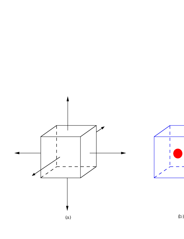
Figure 4.3: (a) The (static) monopole defined on the dual lattice is equivalent to the total magnetic flux of the Dirac string. (b) The neighboring links/plaquettes around the dual link.

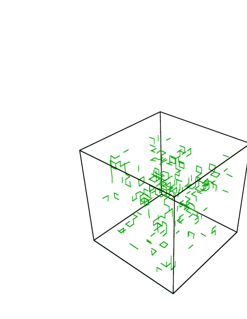
Figure 4.4: The typical example of the 3-dimensional time-slice of the monopole current in the MA gauge in the lattice QCD with $\beta$ = 2.4 on $16^{4}$.

We show in Fig.4.4 a typical example of the monopole current at a time slice in the lattice QCD at $\beta$ = 2.4 in the maximally abelian (MA) gauge. In each gauge configuration, the monopole current appears as a distinct line-like object, and the neighbor of the monopole can be defined on the lattice. However, taking the temporal direction into account, the monopole current forms a global network covering over ${\bf R}^{4}$.

Here, we summarize several relevant properties of $k_{\mu}(s)$.

1. The monopole current $k_{\mu}$ is topologically quantized and $k^{lat}_{\mu}(s)$ takes an integer $k^{lat}_{\mu}(s)$ $\in$ ${\bf Z}$ in the definition of Eq.(4.21). As the result, $k^{lat}_{\mu}(s)$ forms a line-like object in the space-time ${\bf R}^{4}$, since $k^{lat}_{\mu}$ is a conserved current as $\partial_{\mu}k_{\mu}^{lat}=0$. These features of $k_{\mu}^{lat}(s)$ $\in$ ${\bf Z}$ are quite unique and different from the electric current $j_{\mu}(s)$ $\in$ ${\bf R}$, which can spread as a continuous field.

2. In the lattice formalism, $k^{lat}_{\mu}\equiv\frac{1}{2\pi}\partial_{\alpha}^{*}\bar{\theta}_{\alpha\mu}$ is defined as a three-form on the dual link. For the use of the forward derivative, $k^{lat}_{\mu}(s)$ is to be defined on the dual link between $s^{\rm dual}_{\pm\mu}\equiv s+\frac{\hat{x}}{2}+\frac{\hat{y}}{2}+\frac{\hat{z}}{2}+\frac{\hat{t}}{2}\pm\frac{\hat{\mu}}{2}$. For instance, $k^{lat}_{0}(s)$ is placed on the dual link between $(s_{x}+\frac{1}{2},s_{y}+\frac{1}{2},s_{z}+\frac{1}{2},s_{t})$ and $(s_{x}+\frac{1}{2},s_{y}+\frac{1}{2},s_{z}+\frac{1}{2},s_{t}+1)$. Thus, the monopole is defined to appear at the center of the 3-dimensional cube perpendicular to the monopole-current direction as shown in Fig.4.3(b).

3. Because of $k_{\mu}\equiv\partial_{\alpha}^{*}F_{\alpha\mu}=-\frac{1}{2}\varepsilon_{\mu\alpha\beta\gamma}\partial_{\alpha}F_{\beta\gamma}$, $k_{\mu}$ only affects the perpendicular components to the $\hat{\mu}$-direction for the “electric variable” as $F_{\alpha\beta}$ in a direct manner. For instance, the static monopole with $k_{0}\neq 0$ creates the magnetic field $F_{ij}$ ($i,j$=1,2,3) around it, but does not bring the electric field $F_{0i}$. Hence, in testing the field around the monopole in the next chapter, one has to consider the difference between such perpendicular components and others.

We now consider the relationship between the lattice variable and the field variable in the continuum theory. The continuous abelian field ${\cal A}_{\mu}(x)\equiv A^{3}_{\mu}(x)\frac{\tau^{3}}{2}$ is expressed as

$$eA^{3}_{\mu}\equiv\theta^{3}_{\mu}\cdot\frac{2}{a}$$ (4.22)

with the gauge coupling constant $e$ and the lattice spacing $a$. The abelian field strength ${\cal F}_{\mu\nu}(x)\equiv F_{\mu\nu}(x)\frac{\tau^{3}}{2}$ in the continuum theory is written as

$$eF_{\mu\nu} \equiv {\rm mod}_{2\pi}(\theta_{\mu\nu})\cdot\frac{2}{a^{2}}={\bar{\theta}_{\mu\nu}}\cdot\frac{2}{a^{2}},$$ (4.23)

and $F_{\mu\nu}$ is composed of two parts according to the decomposition (4.20)

$$F_{\mu\nu} = (\partial\wedge A^{3})_{\mu\nu}-F^{\rm sing}_{\mu\nu}.$$ (4.24)

Thus, in the SU$(N_{c})$-lattice formalism, the difference between the field strength $F_{\mu\nu}$ and two-form $(\partial\wedge A)_{\mu\nu}$ arises from the periodicity of the angle variable in the compact subgroup U(1)${}^{N_{c}-1}$ embedded in SU($N_{c}$). Here, the singular Dirac-string part $F^{\rm sing}_{\mu\nu}$ is directly related to $2\pi n_{\mu\nu}$ and is written by

$$F^{\rm sing}_{\mu\nu}=2\pi n_{\mu\nu}\cdot\frac{2}{ea^{2}}=\frac{4\pi}{e}n_{\mu\nu}\frac{1}{a^{2}}.$$ (4.25)

Owing to existence of $F^{\rm sing}_{\mu\nu}$ in Eq.(4.24), the monopole current $k_{\mu}(x)\equiv k^{3}_{\mu}(x)\frac{\tau^{3}}{2}\equiv\partial_{\alpha}{}^{*}F_{\alpha\mu}\frac{\tau^{3}}{2}$ appears in the continuum theory and is written as

$$k^{3}_{\mu}=k^{lat}_{\mu}\cdot\frac{4\pi}{ea^{3}}=-\frac{4\pi}{e}\partial_{\alpha}{}^{*}n_{\alpha\mu}\frac{1}{a^{3}},$$ (4.26)

where the magnetic-charge unit $g\equiv\frac{4\pi}{e}$ naturally appears in $k_{\mu}$.

Chapter 5 Large Field Fluctuation around Monopole

In this chapter, we study the QCD-monopole appearing in the abelian gauge in terms of the gluon field fluctuation [45, 55]. For simplicity, we take $N_{c}=2$. In the static frame of the QCD-monopole with the magnetic charge $g$, a spherical “magnetic field” is created around the monopole in the abelian sector of QCD as

$${\bf H}(r)=\frac{g}{4\pi r^{3}}{\bf r}$$ (5.1)

with ${\bf H}_{i}\equiv\varepsilon_{ijk}\partial_{j}A^{3}_{k}$. Thus, the QCD-monopole inevitably accompanies a large fluctuation of the abelian gluon component $A^{3}_{\mu}$ around it. As was discussed in the previous chapter, in the abelian gauge, the formal action of abelian projected QCD or the abelian part of the QCD action is given by $S^{\rm Abel}\equiv-\frac{1}{4}\int d^{4}x\{(\partial_{\mu}A_{\nu}^{3}-\partial_{\nu}A_{\mu}^{3})^{2}-F_{\mu\nu}^{\rm sing}\}$, where $-F_{\mu\nu}^{\rm sing}$ appears and eliminates the Dirac-string contribution. In the abelian part, the field energy created around the monopole is estimated as the ordinary electro-magnetic energy,

$${\cal E}(a)=\int_{a}^{\infty}d^{3}x\frac{1}{2}{\bf H}(r)^{2}=\frac{g^{2}}{8\pi a},$$ (5.2)

where $a$ is an ultraviolet cutoff like a lattice mesh. As the “mesh” $a$ goes to 0, the monopole inevitably accompanies an infinitely large energy-fluctuation in the abelian part and makes $S^{\rm Abel}$ divergent.

Since there seems no plausible reason to eliminate such a divergence via renormalization, the monopole seems difficult to appear in the abelian gauge theory controlled by $S^{\rm Abel}$. This is the reason why QED does not have the point-like Dirac monopole. Then, why can the QCD-monopole appear in abelian projected QCD ? To answer it, let us consider the division of the total QCD action $S^{\rm QCD}$ into the abelian part $S^{\rm Abel}$ and the remaining part $S^{\rm off}\equiv S^{\rm QCD}-S^{\rm Abel}$, which is contribution from the off-diagonal gluon component. While $S^{\rm QCD}$ and $S^{\rm Abel}$ are positive definite in the Euclidean metric, $S^{\rm off}$ is not positive definite and can take a negative value. Then, around the QCD-monopole, the abelian action $S^{\rm Abel}$ should be partially canceled by the remaining contribution $S^{\rm off}$ from the off-diagonal gluon component, so as to keep the total QCD action $S^{\rm QCD}$ finite even for $a\rightarrow 0$. Similar cancellation between the gauge field and the Higgs field fluctuation is also found around the GUT monopole. Thus, we expect large off-diagonal gluon components around the QCD-monopole for its existence as well as a large field fluctuation in the abelian part. Based on this analytical consideration, we study the field fluctuation and monopoles in the MA gauge using the lattice QCD.

5.1 Gluon Field Configuration around Monopoles

We study the properties of monopole in terms of the gluon configuration in the MA gauge. In particular, we investigate the correlation between monopoles and the abelian angle variable $\theta_{\mu}^{3}(s)$ and abelian projection rate $R_{\rm Abel}$.

First, we show the local correlation between the abelian angle variable and the monopole using the gauge configuration in the MA gauge with U(1)₃ Landau gauge in Fig.5.1. The closed symbol denotes the monopole current on the dual link. Around the monopoles, the abelian angle variable tends to fluctuate largely.

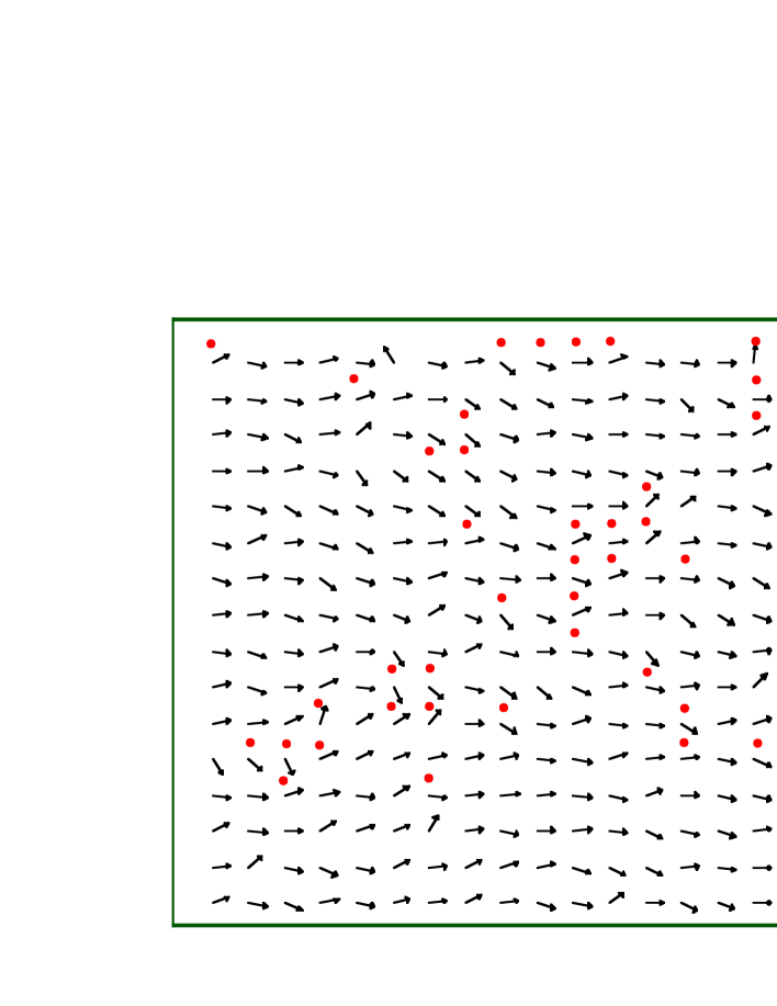
Figure 5.1: The local correlation between the abelian angle variable $\theta_{\mu}^{3}(s)$ and the monopole current $k_{\mu}$ in the MA gauge with U(1)₃ Landau gauge at $\beta=2.4$. The closed symbol denotes the monopole current on the dual link.

Next, we consider the correlation between the field variables and the monopole quantitatively in the lattice QCD. For this argument, one has to recall the property of the monopole current shown in Section 4.3. In particular, one should note that $k_{\mu}(s)$ is defined on the dual link and only affects the perpendicular components to the $\hat{\mu}$-direction for the electric variable as $F_{\alpha\beta}$ because of $k_{\mu}\equiv\partial_{\alpha}^{*}F_{\alpha\mu}=-\frac{1}{2}\varepsilon_{\mu\alpha\beta\gamma}\partial_{\alpha}F_{\beta\gamma}$. Taking account of these properties, we study the local correlation between the field variables and the monopole current $k_{\mu}(s)$ in the MA gauge with the U(1)₃ Landau gauge. We first measure the average of the abelian angle variable $\theta^{3}_{\mu}(s)$ over the neighboring links around the dual link (see Fig.4.3(a)),

$$|\bar{\theta}^{3}(s,\hat{\mu})|\equiv\frac{1}{12}\sum_{\alpha\beta\gamma}\sum_{m,n=0}^{1}\frac{1}{2}|\varepsilon_{\mu\alpha\beta\gamma}|\cdot|\theta^{3}_{\alpha}(s+m\hat{\beta}+n\hat{\gamma})|,$$ (5.3)

which only consists of the perpendicular components considering the above monopole property. Here, the index $\hat{\mu}$ denotes the direction of the dual link, and $|\bar{\theta}^{3}(s,\hat{\mu})|$ corresponds to the average over the 12 sides of the 3-dimensional cube perpendicular to the $\hat{\mu}$-direction [45]. We show in Fig.5.2 the probability distribution $P(|\bar{\theta}^{3}|)$ of $|\bar{\theta}^{3}(s,\hat{\mu})|$ in the MA gauge with the U(1)₃ Landau gauge at $\beta=2.4$. The solid curve denotes $P(|\bar{\theta}^{3}|)$ around the monopole current, while the dashed curve denotes the total distribution on the whole lattice. The abelian angle variable $|\theta^{3}_{\mu}(s)|$ takes a large value around the monopole. In other words, the monopole provides the large fluctuation of the abelian gauge field, which would enhance the randomness of the abelian link variable.

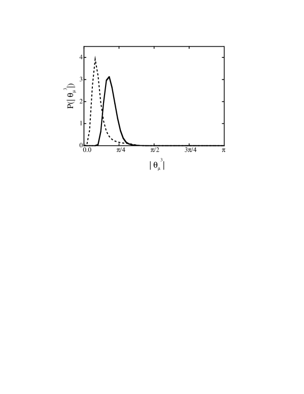
Figure 5.2: The solid curve denotes the probability distribution $P(|\bar{\theta}^{3}|)$ of the averaged abelian angle variable $|\bar{\theta}^{3}(s,\hat{\mu})|$ around the monopole current in the MA gauge with the U(1)₃ Landau gauge fixing. Here, $|\bar{\theta}^{3}(s,\hat{\mu})|$ is the average of $|\theta_{\alpha}^{3}(s)|$ over the neighboring links around the dual link, For comparison, the total distribution $P$ on the whole lattice is also added by the dashed curve. Around the monopole, $|\bar{\theta}^{3}|$ corresponding to the abelian gluon component takes a large value.

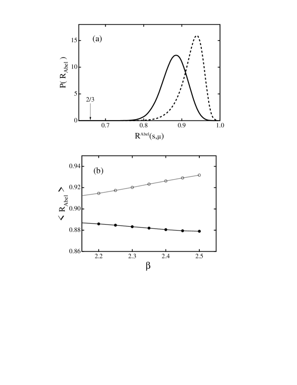
Figure 5.3: (a) The solid curve denotes the probability distribution $P(\bar{R}_{\rm Abel})$ of the averaged abelian projection rate $\bar{R}_{\rm Abel}(s,\hat{\mu})$ around the monopole current in the MA gauge in the SU(2) lattice QCD with $\beta=2.4$ on $16^{4}$. For comparison, the total distribution $P$ on the whole lattice is also added by the dashed curve. (b) The solid curve denotes abelian projection rate $\langle\bar{R}_{\rm Abel}\rangle$ around the monopole current in the MA gauge as the function of $\beta$. The dashed curve denotes $\langle\bar{R}_{\rm Abel}\rangle$ on the whole lattice.

Similar to $|\bar{\theta}^{3}(s,\hat{\mu})|$, we measure the average $\bar{R}_{\rm Abel}$ of the abelian projection rate $R_{\rm Abel}(s,\hat{\mu})\equiv\cos\theta_{\mu}(s)$ over the neighboring links around the dual link,

$$\bar{R}_{\rm Abel}(s,\hat{\mu})\equiv\frac{1}{12}\sum_{\alpha\beta\gamma}\sum_{m,n=0}^{1}\frac{1}{2}|\varepsilon_{\mu\alpha\beta\gamma}|\cos\theta_{\alpha}(s+m\hat{\beta}+n\hat{\gamma})$$ (5.4)

in the MA gauge to investigate the correlation between off-diagonal gluons and monopoles. As shown in Fig.5.3(a), $\bar{R}_{\rm Abel}$ around the monopole current becomes smaller than the total average of $\bar{R}_{\rm Abel}$ and therefore the magnitude of the off-diagonal gluon component becomes larger around the monopole. The $\beta$ dependence of the abelian projection rate $\langle R_{\rm Abel}\rangle$ is shown in Fig.5.3(b). Although $\langle R_{\rm Abel}\rangle$ on the whole lattice approaches to unity as $\beta\rightarrow\infty$, $\langle R_{\rm Abel}\rangle$ around the monopole is about 0.88 and is not changed even in the large $\beta$ region. Thus, the monopole provides the large fluctuation both for the abelian field and for the off-diagonal gluon.

5.2 Plaquette Action Density around Monopoles

We next study monopoles in terms of the plaquette action density. We define the SU(2), abelian and “off-diagonal” plaquette action densities as

$$S^{\rm SU(2)}_{\mu\nu}(s) \equiv 1-\frac{1}{2}{\rm tr}\Box^{\rm SU(2)}_{\mu\nu}(s),$$ (5.5)

$$S^{\rm Abel}_{\mu\nu}(s) \equiv 1-\frac{1}{2}{\rm tr}\Box^{\rm Abel}_{\mu\nu}(s),$$ (5.6)

$$S^{\rm off}_{\mu\nu}(s) \equiv S^{\rm SU(2)}_{\mu\nu}(s)-S^{\rm Abel}_{\mu\nu}(s),$$ (5.7)

where $\Box^{\rm SU(2)}_{\mu\nu}(s)$ and $\Box^{\rm Abel}_{\mu\nu}(s)$ denote the SU(2) and the abelian plaquette variables, respectively;

$$\Box^{\rm SU(2)}_{\mu\nu}(s) \equiv U_{\mu}(s)U_{\nu}(s+\hat{\mu})U^{\dagger}_{\mu}(s+\hat{\nu})U^{\dagger}_{\nu}(s),$$ (5.8)

$$\Box^{\rm Abel}_{\mu\nu}(s) \equiv u_{\mu}(s)u_{\nu}(s+\hat{\mu})u^{\dagger}_{\mu}(s+\hat{\nu})u^{\dagger}_{\nu}(s).$$ (5.9)

Here, all of $S_{\mu\nu}$ are defined as symmetric tensors, $S_{\mu\nu}=S_{\nu\mu}$, instead of the Lorentz scalar, considering the above property of the monopole current. In the continuum limit $a\rightarrow 0$, $S^{\rm SU(2)}_{\mu\nu}(s)$ and $S^{\rm Abel}_{\mu\nu}(s)$ are related to the SU(2) and the abelian action densities as $S^{\rm SU(2)}_{\mu\nu}(s)\rightarrow\frac{1}{4}a^{4}e^{2}{\rm tr}G^{2}_{\mu\nu}$ and $S^{\rm Abel}_{\mu\nu}(s)\rightarrow\frac{1}{4}a^{4}e^{2}{\rm tr}{\cal F}^{2}_{\mu\nu}$, and then we call $S_{\mu\nu}$ as the action density, in spite of the lack of the summation on the Lorentz indices. Here, $S^{\rm off}_{\mu\nu}$ corresponds to the contribution of the off-diagonal gluon. While $S^{\rm SU(2)}_{\mu\nu}$ and $S^{\rm Abel}_{\mu\nu}$ are positive-definite, $S^{\rm off}_{\mu\nu}$ is not positive-definite and can take a negative value.

In order to examine the correlation between the action densities and the monopole current defined on the dual link, we measure the average of the action density $S(s)$ over the neighboring plaquettes around the dual link,

$$\bar{S}(s,\hat{\mu})\equiv\frac{1}{6}\sum_{\alpha\beta\gamma}\sum_{m=0}^{1}\frac{1}{2}|\varepsilon_{\mu\alpha\beta\gamma}|S_{\alpha\beta}(s+m\hat{\gamma}).$$ (5.10)

Here, $\hat{\mu}$ appearing in $\bar{S}(s,\hat{\mu})$ denotes the direction of the dual link, and $\bar{S}(s,\hat{\mu})$ corresponds to the average over 6 faces of the 3-dimensional cube perpendicular to the $\hat{\mu}$-direction.

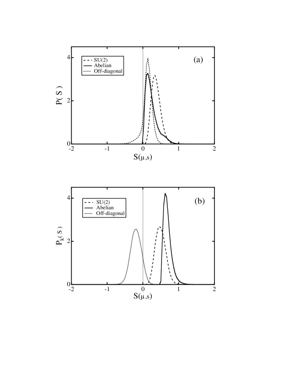
Figure 5.4: (a) The probability distribution $P(\bar{S})$ of density $\bar{S}(s,\hat{\mu})$ on the whole lattice in the MA gauge at $\beta=2.4$ on $16^{4}$ lattice. (b)The probability distribution $P_{k}(\bar{S})$ of the action density $\bar{S}(s,\hat{\mu})$ around the monopole current ${k_{\mu}}$. The dotted and the solid curves denote $P(\bar{S}^{\rm SU(2)})$ and $P(\bar{S}^{\rm Abel})$, respectively. The dashed curve denotes $P(\bar{S}^{\rm off})$ for the off-diagonal part $\bar{S}^{\rm off}$ of the action density.

Figure 5.5: The action density as the function of $\beta$ in the MA gauge in the SU(2) lattice QCD. The closed symbols denote the action densities $\langle S\rangle$ around the monopole current, while the open symbols denote those on the whole lattice. The square, circle and rhombus denote $\langle S^{\rm SU(2)}\rangle$, $\langle S^{\rm Abel}\rangle$ and $\langle S^{\rm off}\rangle$, respectively. The monopole accompanies a large U(1)₃ plaquette action, however, such a large U(1)₃ action is strongly canceled by the off-diagonal part.

We show in Fig.5.4 the probability distribution $P(\bar{S})$ of the action densities $\bar{S}(s,\hat{\mu})$ in the SU(2), the abelian and the off-diagonal parts. Before the argument around the monopole current, we show the action densities on the whole lattice in Fig.5.4 (a). On the whole lattice, most $\bar{S}^{\rm off}$ are positive, and both $\bar{S}^{\rm Abel}$ and $\bar{S}^{\rm off}$ tend to take smaller values than $\bar{S}^{\rm SU(2)}=\bar{S}^{\rm Abel}+\bar{S}^{\rm off}$. In other words, $\bar{S}^{\rm Abel}$ and positive $\bar{S}^{\rm off}$ additionally contribute to $\bar{S}^{\rm SU(2)}$.

However, such a tendency of the action densities is drastically changed around the monopole as shown in Fig.5.4(b). We find remarkable features of the action densities around the monopole as follows.

1. Around monopoles, most $\bar{S}^{\rm off}$ take negative values, and $\bar{S}^{\rm Abel}$ is larger than $\bar{S}^{\rm SU(2)}=\bar{S}^{\rm Abel}+\bar{S}^{\rm off}$.

2. Due to the cancellation between $\bar{S}^{\rm Abel}$ and $\bar{S}^{\rm off}$, $\bar{S}^{\rm SU(2)}$ does not take an extremely large value around the monopole.

Thus, the large abelian action density $S^{\rm Abel}$ around the monopole is strongly canceled by the off-diagonal contribution $S^{\rm off}$ to keep the total QCD action $S^{\rm QCD}=S^{\rm Abel}+S^{\rm off}$ small. Here, different from $S^{\rm SU(2)}$, $S^{\rm Abel}$ itself does not control the system directly, and hence there is no severe constraint from $S^{\rm Abel}$. However, large $S^{\rm Abel}$ is still not preferable, because the large-cancellation requirement between $S^{\rm Abel}$ and $S^{\rm off}$ leads to a strong constraint on the off-diagonal gluon and brings the strong reduction of the configuration number.

Around the monopole, the abelian action density $S^{\rm Abel}$ takes a large value, and this value can be estimated from a following simple calculation. Without loss of generality, the monopole-current direction is locally set to be parallel to the temporal direction as $k^{lat}_{0}(s)\equiv\frac{1}{2\pi}\partial_{\alpha}{}^{*}{\bar{\theta}_{\alpha 0}}(s)=\pm 1$. Here, $k_{0}^{lat}(s)$ is expressed as the sum of six plaquette variables $\bar{\theta}_{ij}$ ($i,j$=1,2,3) around the monopole, because of $k_{0}^{lat}(s)=-\frac{1}{4\pi}\varepsilon_{ijk}\partial_{i}\bar{\theta}_{jk}(s)=-\frac{1}{2\pi}\sum_{i}\sum_{j<k}\varepsilon_{ijk}\{\bar{\theta}_{jk}(s+\hat{i})-\bar{\theta}_{jk}(s)\}$. Hence, the total sum of six $|\bar{\theta}_{ij}(s)|(i<j)$ is to exceed $2\pi$ to realize $k_{0}(s)=\pm 1$. Since large $|\bar{\theta}_{ij(s)}|$ accompanying large $S^{\rm Abel}$ is not preferable, the magnetic field $|\bar{\theta}_{ij}|$ around the monopole is estimated as $|\bar{\theta}_{ij}|\simeq 2\pi/6=\pi/3$ on the average, using the spherical symmetry of the magnetic field in the vicinity of the monopole. Accordingly, we estimate as $S^{\rm Abel}_{ij}=1-{\rm cos}(|\bar{\theta}_{ij}|)\simeq 1-\cos\frac{\pi}{3}=\frac{1}{2}$ around the monopole on the average. The above argument can be easily generalized to the case with arbitrary monopole-current direction.

Then, existence of monopoles brings a peak around $S^{\rm Abel}=\frac{1}{2}$ in the distribution $P(S^{\rm Abel})$. In fact, the abelian action density $S^{\rm Abel}$ has two ingredients; one is nontrivial large fluctuation about $S^{\rm Abel}=1/2$ originated from the monopole, and the other is remaining small fluctuations, which is expected to vanish as $S^{\rm Abel}\rightarrow 0$ as $a\rightarrow 0$. As shown in Fig.5.5, the peak originated from the monopole is almost $\beta$ independent, while the other fluctuation becomes small for large $\beta$. At a glance from this result, the monopole seems hard to exist at the small mesh $a$, since the monopole needs a large abelian action $S^{\rm Abel}$. Nevertheless, the monopole can exist in QCD even in the large $\beta$ region owing to the contribution of the off-diagonal gluon. As shown in Fig.5.4(b), the off-diagonal part $S^{\rm off}$ of the action density around the monopole tends to take a large negative value, and strongly cancels with the large abelian action $S^{\rm Abel}$ to keep the total SU(2) action $S^{\rm QCD}$ finite.

Here, we consider the angle variable $\tilde{\chi}_{\mu}(x)$ of the off-diagonal gluons $A_{\mu}^{\pm}(x)$ around the monopole. In the MA gauge, the amplitude of $A_{\mu}^{\pm}(x)$ is strongly reduced, and $\tilde{\chi}_{\mu}(x)$ can be approximated as a random variable on the whole, because $\tilde{\chi}_{\mu}(x)$ is free from the MA gauge condition entirely and is less constrained from the QCD action due to the small $|A_{\mu}^{\pm}(x)|$. However, around the monopole, the off-diagonal gluon $A_{\mu}^{\pm}(x)$ inevitably has a large amplitude even in the MA gauge to cancel the large abelian action density. This requirement on the reduction of the total action density severely constrains the randomness of the angle variable $\tilde{\chi}_{\mu}(x)$ of the off-diagonal gluon $A_{\mu}^{\pm}(x)$ around the monopole. As the result, the randomness of $\tilde{\chi}_{\mu}(x)$ is weaken, and continuity of $\tilde{\chi}_{\mu}(x)$ or $A_{\mu}^{\pm}(x)$ becomes clear in the vicinity of the monopole even in the MA gauge. This continuity of $A_{\mu}^{\pm}(x)$ around the monopole ensures the topological stability of the monopole itself as $\Pi_{2}({\rm SU}(2)/{\rm U}(1))={\bf Z}_{\infty}$.

To summarize, existence of the monopole inevitably accompanies a large abelian plaquette action $S^{\rm Abel}$ around it, however, the off-diagonal part $S^{\rm off}$ takes a large negative value around the monopole and strongly cancels with $S^{\rm Abel}$ to keep $S^{\rm QCD}$ not so large. Due to this strong cancellation between $S^{\rm Abel}$ and $S^{\rm off}$, monopoles can appear in the abelian sector in QCD without large cost of the QCD action $S^{\rm QCD}$, which controls the generating probability of the gluon configuration. The extension of the off-diagonal rich region around the monopole can be interpreted as the effective size or the structure of the monopole, because the abelian gauge theory is largely modified inside the QCD-monopole like the ’t Hooft-Polyakov monopole.

Finally, in this section, let us consider the correlation between monopoles and instantons [39] in terms of the gluon-field fluctuation. The instanton is a nontrivial classical solution of the Euclidean Yang-Mills theory, corresponding to the homotopy group $\Pi_{3}({\rm SU}(N_{c}))={\bf Z}_{\infty}$ [7, 8, 9]. For the instanton, the SU(2) structure of the gluon field is necessary at least. In spite of the difference on the topological origin, recent studies indicate the strong correlation between monopoles and instantons in the QCD vacuum in the MA gauge [38, 40]. What is the origin of the relation between two different topological objects, monopoles and instantons ? In the MA gauge, off-diagonal components are forced to be small, and the gluon field configuration seems abelian on the whole. However, even in the MA gauge, off-diagonal gluons largely remain around the QCD-monopole. The concentration of off-diagonal gluons around monopoles leads to the local correlation between monopoles and instantons: instantons appear around the monopole world-line in the MA gauge, because instantons need full SU(2) gluon components for existence.

Chapter 6 Monopole Projection and Scaling Properties in the MA Gauge

6.1 Decomposition into Monopole and Photon Angle-Variables

Abelian projected QCD is obtained by neglecting the off-diagonal gluon component in the abelian gauge, and it includes both the electric current $j_{\mu}$ and the monopole current $k_{\mu}$. Here, $j_{\mu}$ is generated by charged gluons, and $k_{\mu}$ is generated by the singular SU(2) gauge transformation in the abelian gauge. In the lattice formalism, the U(1)₃-gauge field can be separated into the “monopole part” and the “photon part” using the Coulomb propagator. Here, the monopole part only includes the monopole current $k_{\mu}$ and reproduces the purely linear part of the static quark potential [56]. On the other hand, the photon part includes the electric current $j_{\mu}$ only, and provides the Coulomb potential between the quark and the anti-quark, similarly in the ordinary QED. In this section, we extract the monopole contribution from abelian projected QCD using the lattice Coulomb propagator [54], and study the role of the monopole for confinement.

The abelian gauge field $\theta^{3}_{\mu}(s)$ can be decomposed into the monopole part $\theta^{\rm Mo}_{\mu}(s)$ and the photon part $\theta^{\rm Ph}_{\mu}(s)$ [28],

$$\theta^{\rm Mo}_{\mu}(s) \equiv 2\pi\sum_{s^{\prime}}\langle s|\partial^{-2}|s^{\prime}\rangle\partial_{\alpha}n_{\alpha\mu}(s^{\prime}),$$ (6.1)

$$\theta^{\rm Ph}_{\mu}(s) \equiv \sum_{s^{\prime}}\langle s|\partial^{-2}|s^{\prime}\rangle\partial_{\alpha}\bar{\theta}_{\alpha\mu}(s^{\prime}),$$ (6.2)

where $\langle s|\partial^{-2}|s^{\prime}\rangle=-\frac{1}{4\pi}\frac{1}{(s-s^{\prime})^{2}}$ is the Coulomb propagator in the 4-dimensional Euclidean space. As for the U(1)₃ gauge invariance, $\theta^{\rm Mo}_{\mu}(s)$ is gauge-variant, since $2\pi n_{\mu\nu}$ is gauge-variant. On the other hand, $\theta^{\rm Ph}_{\mu}(s)$ is U(1)₃ gauge-invariant, since it is composed of gauge-invariant $\bar{\theta}_{\mu\nu}$. In the Landau gauge $\partial_{\mu}\theta^{3}_{\mu}(s)=0$, one finds

$$\theta^{\rm Mo}_{\mu}(s)+\theta^{\rm Ph}_{\mu}(s)=\theta_{\mu}^{3}(s).$$ (6.3)

Here, we investigate properties of the monopole and the photon parts in terms of the electric and the magnetic currents. The two form of these angle variables are written as

$$(\partial\wedge\theta^{\rm Mo})_{\mu\nu} ={\bar{\theta}^{\rm Mo}_{\mu\nu}}+2\pi n_{\mu\nu}^{\rm Mo}\hskip 8.5359pt\mbox{with}\hskip 8.5359pt \bar{\theta}^{\rm Mo}_{\mu\nu}={\rm mod}_{2\pi}(\partial\wedge\theta^{\rm Mo})_{\mu\nu}\in(-\pi,\pi]$$

$$(\partial\wedge\theta^{\rm Ph})_{\mu\nu} ={\bar{\theta}^{\rm Ph}_{\mu\nu}}+2\pi n_{\mu\nu}^{\rm Ph}\hskip 8.5359pt\mbox{with}\hskip 8.5359pt \bar{\theta}^{\rm Ph}_{\mu\nu}={\rm mod}_{2\pi}(\partial\wedge\theta^{\rm Ph})_{\mu\nu}\in(-\pi,\pi],$$

using $n_{\mu\nu}^{\rm Mo}$, $n_{\mu\nu}^{\rm Ph}\in{\bf Z}$. The monopole current $k_{\mu}(s)$ and the electric current $j_{\mu}(s)$ in the monopole part are defined as

$$k^{\rm Mo}_{\mu}\equiv\frac{1}{2\pi}\partial_{\alpha}^{*}{\bar{\theta}_{\alpha\mu}^{\rm Mo}}=-\partial_{\alpha}^{*}n^{\rm Mo}_{\alpha\mu},\hskip 28.45274ptj^{\rm Mo}_{\mu}\equiv\partial_{\alpha}{\bar{\theta}^{\rm Mo}_{\alpha\mu}},$$ (6.4)

and those in the photon part are defined as

$$k^{\rm Ph}_{\mu}\equiv\frac{1}{2\pi}\partial_{\alpha}^{*}{\bar{\theta}_{\alpha\mu}^{\rm Ph}}=-\partial_{\alpha}^{*}n^{\rm Ph}_{\alpha\mu},\hskip 28.45274ptj^{\rm Ph}_{\mu}\equiv\partial_{\alpha}{\bar{\theta}^{\rm Ph}_{\alpha\mu}}.$$ (6.5)

From the physical point of view, the decomposition of the abelian sector into the photon and monopole sectors directly corresponds to the separation of the electric current $j_{\mu}$ and the monopole current $k_{\mu}$ near the continuum limit.

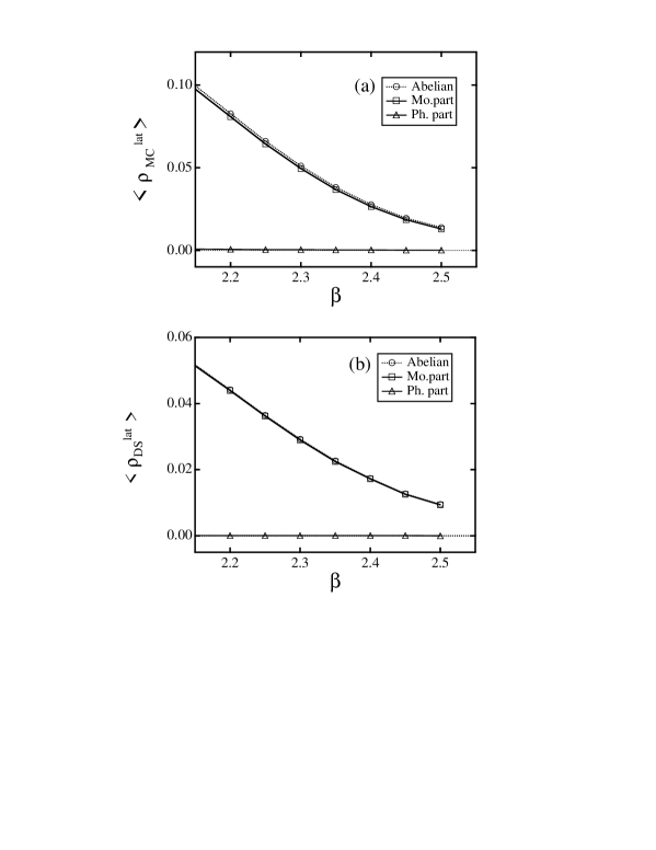
Figure 6.1: (a) The monopole-current density $\rho^{lat}_{\rm MC}$ in the MA gauge as the function of $\beta$. The circle, square and triangle denote $\rho^{lat}_{\rm MC}$ in the abelian, monopole and photon sectors, respectively. (b) The Dirac-sheet density $\rho_{\rm DS}^{lat}$ in the MA gauge with U(1)₃ Landau-gauge as the function of $\beta$. The circle, square and triangle denote $\rho_{\rm DS}^{lat}$ in the abelian, monopole and photon sectors, respectively.

In the actual lattice simulation, we can observe $k_{\mu}^{\rm ph}\simeq 0$, $j_{\mu}^{\rm ph}=j_{\mu}$ and $k^{\rm Mo}_{\mu}\simeq 0$, $k_{\mu}^{\rm Mo}=k_{\mu}$ in the MA gauge within a few percent error for large $\beta$. For instance, we show in Fig.6.1(a) the lattice result of the monopole current density $\rho^{lat}_{\rm MC}\equiv\sum_{s\mu}|k_{\mu}(s)|/\sum_{s\mu}1$ in the MA gauge. One fined $\rho^{\rm Abel}_{\rm MC}\simeq\rho^{\rm Mo}_{\rm MC}$ and $\rho^{\rm Ph}_{\rm MC}\simeq 0$.

Existence of the monopole accompanies the Dirac string. We show also the Dirac-sheet density $\rho_{DS}\equiv\sum_{s\mu\nu}|n_{\mu}(s)|/\sum_{s\mu\nu}1$ in the MA gauge with U(1)₃-Landau gauge in Fig.6.1(b). Owing to the U(1)₃-Landau gauge fixing, the abelian angle variable $\theta^{3}_{\mu}$ becomes mostly continuous and $|(\partial\wedge\theta^{3})_{\mu\nu}|$ scarcely exceeds $\pi$, so that redundant Dirac sheets are eliminated and the correlation between $\rho_{\rm MC}^{lat}$ and $\rho_{\rm DS}^{lat}$ appears. More quantitative argument of $\rho_{\rm MC}^{lat}$ and $\rho_{\rm DS}^{lat}$ will be done in the physical unit in Section 6.4.

For comparison, we investigate the monopole density $\rho_{\rm MC}^{lat}$ in the SU(2) Landau gauge with SU(2)/U(1)₃ fixed, which is a kind of the abelian gauge. In the SU(2) Landau gauge, each component of the gluon field is maximally smooth, and monopoles scarcely appear because they are generated from the singular-like large fluctuation of the abelian field. For instance, $\rho_{\rm MC}^{lat}$ in the SU(2) Landau gauge in less than 1/10 of $\rho_{\rm MC}^{lat}$ in the MA gauge at $\beta=2.4$. In fact, in the regular SU(2) gauge configuration, the gluon fluctuation is shared into each component almost equivalently, and there appears no singularity as the monopole due to the “wise sharing” of the fluctuation. On the other hand, in the MA gauge, large gluon fluctuations are concentrated into the abelian sector by the suppression of off-diagonal gluon components, and therefore the monopole appears as the singularity or the topological defect from the large field fluctuation in the abelian sector.

6.2 Link and Plaquette Variables in Monopole and Photon Sectors

In general, confinement observed as the area-low reduction of the Wilson loop is closely related to the large gluon fluctuation as is suggested by the strong coupling QCD. Hence, from monopole dominance for the confinement force observed on the lattice, one may expect large fluctuation of the gluon field in the monopole sector and small ones in the photon sector. This naive expectation on the large fluctuation $\theta_{\mu}^{\rm Mo}$ may be also suggested from the definition of $\theta_{\mu}^{\rm Mo}$ and $\theta_{\mu}^{\rm Ph}$ in Eq.(6.3), since the monopole angle variable $\theta_{\mu}^{\rm Mo}$ consists of the integer part $2\pi n$ $\in$ $2\pi{\bf Z}$, while the photon angle variable $\theta^{\rm Ph}_{\mu}$ consists of the fractional part $\bar{\theta}_{\mu}$ $\in$ $[-\pi,\pi)$. We measure the lattice angle variables $\theta^{3}_{\mu}(s)$, $\theta^{\rm Mo}_{\mu}(s)$ and $\theta^{\rm Ph}_{\mu}(s)$ in the MA gauge with U(1)₃ Landau gauge as shown in Fig.6.2. On the whole shape of the probability distribution $P(\theta_{\mu})$ of link variable, the distribution of monopole part $P(\theta_{\mu}^{\rm Mo})$ is smaller than that of the photon part $P(\theta_{\mu}^{\rm Ph})$, and $P(\theta_{\mu}^{3})$ is similar to $P(\theta_{\mu}^{\rm Ph})$ rather than $P(\theta_{\mu}^{\rm Mo})$. These results are in contradiction to the above expectation on the large fluctuation of $P(\theta_{\mu}^{\rm Mo})$, and seem to be surprising in terms of the confinement properties, because the string tension in the abelian sector resembles that in the monopole sector and the string tension in the photon sector is almost zero.

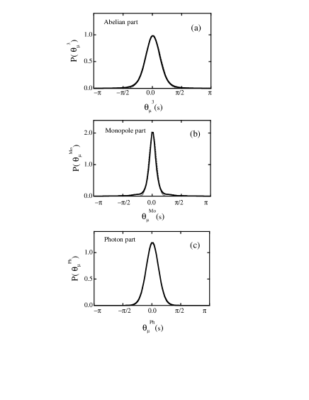
Figure 6.2: The probability distribution $P(\theta_{\mu})$ of lattice angle variables $\theta^{3}_{\mu}(s)$, $\theta^{\rm Mo}_{\mu}(s)$, $\theta^{\rm Ph}_{\mu}(s)\in(-\pi,\pi]$ in the MA gauge with the U(1)₃ Landau gauge fixing at $\beta=2.4$ on $16^{4}$ lattice. (a) the abelian angle variable $P(\theta^{3}_{\mu})$. (b) the monopole angle variable $P(\theta^{\rm Mo}_{\mu})$. (c) the photon angle variable $P(\theta^{\rm Ph}_{\mu})$. The dotted curves are fitting Gaussian curves in Eq.(6.6) with $\alpha=$0.167 for $P(\theta^{3}_{\mu})$, $\alpha=$0.038 for $P(\theta^{\rm Mo}_{\mu})$ and $\alpha=$0.114 for $P(\theta^{\rm Ph}_{\mu})$.

Quantitatively, the whole shape of probability distributions $P(\theta_{\mu}^{\rm 3})$, $P(\theta_{\mu}^{\rm Mo})$ and $P(\theta_{\mu}^{\rm Ph})$ can be fitted with the Gaussian curve around $\theta=0$ as

$$P(\theta)=\frac{1}{\sqrt{2\alpha\pi}}e^{-\frac{1}{2\alpha}\theta^{2}}$$ (6.6)

with $\alpha=$0.167 for $P(\theta^{3}_{\mu})$, $\alpha=$0.038 for $P(\theta^{\rm Mo}_{\mu})$ and $\alpha=$0.114 for $P(\theta^{\rm Ph}_{\mu})$.

Now let us reconsider the fluctuation of the monopole part. In the U(1)₃ Landau gauge, the appearance of the Dirac sheet with $n_{\mu\nu}\neq 0$ is strongly suppressed, because the field is forced to be continuous there. Therefore, almost all of the two form $\theta_{\mu\nu}^{\rm Mo}\equiv\partial_{\mu}\theta_{\nu}^{\rm Mo}-\partial_{\nu}\theta_{\mu}^{\rm Mo}$ satisfies $-\pi<\theta_{\mu\nu}^{\rm Mo}\leq\pi$, i.e., one finds $n_{\mu\nu}^{\rm Mo}(s)=0$ almost everywhere on the lattice. This is the reason why the fluctuation of the monopole angle variable $\theta^{\rm Mo}_{\mu}$ becomes small. However, there appears the relic of the large fluctuation of the abelian angle variable in the monopole angle variable, as shown in Fig.6.3. Similar to $P(\theta^{3}_{\mu})$, the distribution $P(\theta^{\rm Mo}_{\mu})$ of the monopole angle variable has a non-Gaussian large tail even for $|\theta^{\rm Mo}|\leq\frac{\pi}{2}$, while $P(\theta^{\rm Ph}_{\mu})$ has the Gaussian tail only and mainly distributes within $-\frac{\pi}{2}<\theta^{\rm Ph}_{\mu}<\frac{\pi}{2}$ as shown in Fig.6.3. Such a large fluctuation of $\theta^{\rm Mo}_{\mu}$ is responsible for the appearance of the monopole, and it also would play a relevant role for confinement properties, because a large reduction of the string tension is observed in the lattice QCD by the artificial elimination of the large fluctuation.

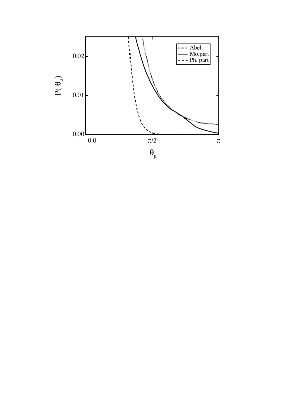
Figure 6.3: The tail of $P(\theta^{3}_{\mu})$, $P(\theta^{\rm Mo}_{\mu})$ and $P(\theta^{\rm Ph}_{\mu})$. Both $P(\theta^{\rm 3}_{\mu})$ and $P(\theta^{\rm Mo}_{\mu})$ include a large fluctuation ingredient as $\theta_{\mu}>\frac{\pi}{2}$, while $P(\theta^{\rm Ph}_{\mu})$ does not have such a large fluctuation ingredient.

Next, we consider the plaquette action densities of the monopole and the photon parts,

$$S^{\rm Mo}_{\mu\nu}(s) \equiv 1-\frac{1}{2}{\rm tr}\Box^{\rm Mo}_{\mu\nu}(s),$$ (6.7)

$$S^{\rm Ph}_{\mu\nu}(s) \equiv 1-\frac{1}{2}{\rm tr}\Box^{\rm Ph}_{\mu\nu}(s),$$ (6.8)

similar to the SU(2) and abelian action densities in Eqs.(5.5) and (5.6). Here, $\Box^{\rm Mo}_{\mu\nu}(s)$ and $\Box^{\rm Ph}_{\mu\nu}(s)$ are the plaquette variables in the monopole and photon parts,

$$\Box^{\rm Mo}_{\mu\nu}(s) \equiv u^{\rm Mo}_{\mu}(s)u_{\nu}^{\rm Mo}(s+\hat{\mu})u^{{\rm Mo}\dagger}_{\mu}(s+\hat{\nu})u^{{\rm Mo}\dagger}_{\nu}(s),$$ (6.9)

$$\Box^{\rm Ph}_{\mu\nu}(s) \equiv u^{\rm Ph}_{\mu}(s)u_{\nu}^{\rm Ph}(s+\hat{\mu})u^{{\rm Ph}\dagger}_{\mu}(s+\hat{\nu})u^{{\rm Ph}\dagger}_{\nu}(s),$$ (6.10)

respectively. To see the monopole effect on the action density $S_{\mu\nu}(s)$, we measure the average $\bar{S}(s,\mu)$ over the neighboring plaquettes around the dual link,

$$\bar{S}(s,\hat{\mu})\equiv\frac{1}{6}\sum_{\alpha\beta\gamma}\sum_{m=0}^{1}\frac{1}{2}|\varepsilon_{\mu\alpha\beta\gamma}|S_{\alpha\beta}(s+m\hat{\gamma}),$$ (6.11)

similar to Eq.(5.10). As shown in Fig.6.4, both action densities $P(S^{\rm Mo})$ and $P(S^{\rm Ph})$ have a peak near $S=0$. For the monopole parts, there are two ingredients in the probability distribution $P(S^{\rm Mo})$ of the monopole action density $S^{\rm Mo}(s,\mu)$: one is the large fluctuation around $S^{\rm Mo}=\frac{1}{2}$ and the other is the small fluctuation near $S^{\rm Mo}\simeq 0$. The large fluctuation ingredient corresponds to the average action-density over six plaquettes of the cube including the monopole inside

$$S_{\mu\nu}^{\rm Mo}=1-\frac{1}{2}{\rm tr}\Box_{\mu\nu}^{\rm Mo}=1-\cos\bar{\theta}_{\mu\nu}^{\rm Mo}\simeq 1-\cos\frac{2\pi}{6}=\frac{1}{2},$$ (6.12)

which is similar to the abelian action density $P(S^{\rm Abel})$ around the monopole, as shown in Fig.5.4. Here, $2\pi$ is the total magnetic flux created by the unite charge monopole. On the other hand, the small fluctuation ingredient corresponds to the plaquette apart from the monopole. For the photon part, the global shape of the probability distribution $P(S^{\rm Ph})$ of the photon action density $S^{\rm Ph}(s,\hat{\mu})$ resembles $P(S^{\rm Abel})$ as shown in Fig.5.4, however, $P(S^{\rm Ph})$ does not have the large fluctuation peak around $S^{\rm Ph}=\frac{1}{2}$, corresponding to the absence of the monopole unlike $P(S^{\rm Abel})$. In the distribution $P(S^{\rm Mo})$, the peak position around $S^{\rm Mo}=\frac{1}{2}$ is almost $\beta$-independent, since it is geometrically determined as Eq.(6.12). On the other hand, the peak near $S=0$ becomes narrow both in $P(S^{\rm Mo})$ and in $P(S^{\rm Ph})$ as $\beta$ increases.

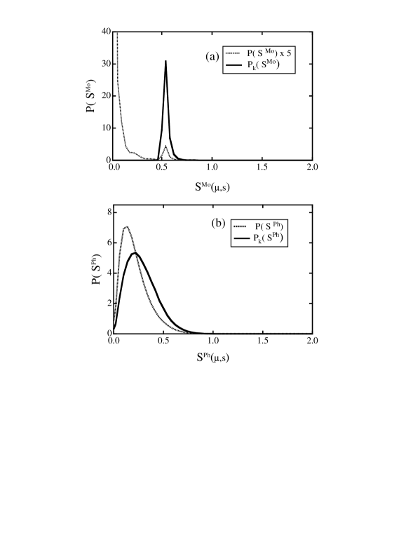
Figure 6.4: (a) The probability distribution $P(S^{\rm Mo})$ of the monopole part of the action density $S^{\rm Mo}(s,\hat{\mu})$ around the monopole. The dotted curve denotes $S^{\rm Mo}(s,\hat{\mu})$ on the whole lattice. The value of $S^{\rm Mo}(s,\hat{\mu})$ is the average of the action density $S^{\rm Mo}_{\mu\nu}(s)$ over the neighboring plaquettes around the dual link. (b) The probability distribution $P(S^{\rm Ph})$ of the photon part of action density $S^{\rm Ph}(s,\hat{\mu})$ around the monopole. The dotted curve denotes $S^{\rm Ph}(s,\hat{\mu})$ on the whole lattice.

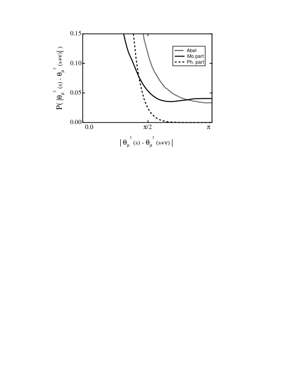
Figure 6.5: The probability distribution of the derivative of the lattice angle variables. The dashed, solid and dotted curves denote $P(|\theta^{3}_{\mu}(s)-\theta^{3}_{\mu}(s+\hat{\nu})|)$, $P(|\theta^{\rm Mo}_{\mu}(s)-\theta^{\rm Mo}_{\mu}(s+\hat{\nu})|)$ and $P(|\theta^{\rm Ph}_{\mu}(s)-\theta^{\rm Ph}_{\mu}(s+\hat{\nu})|)$, respectively.

Finally in this section, we consider also the monopole effect on the discontinuity of the angle variables. As the result of the large fluctuation of the monopole plaquette variable around the monopole as $S^{\rm Mo}\simeq\frac{1}{2}$, there appears the discontinuity of the link variable $\theta_{\mu}^{\rm Mo}$. We measure the correlation neighboring links $u_{\mu}(s)=e^{i\theta(s)}$ and $u_{\mu}(s+\hat{\nu})=e^{i\theta(s+\hat{\nu})}$. We show in Fig.6.5 the angle difference $\Delta\equiv|{\rm mod}_{2\pi}(\theta_{\mu}(s)-\theta_{\mu}(s+\hat{\nu}))|$ with $\mu\neq\nu$. The photon angle variable $\theta_{\mu}^{\rm Ph}(s)$ tends to be continuous with the only small difference between the neighboring links as $\Delta\leq\frac{\pi}{2}$. This tendency on the continuity of $\theta^{\rm Ph}(s)$ becomes clear as $\beta$ increases. On the other hand, similar to the abelian sector, the monopole angle variable $\theta^{\rm Mo}_{\mu}(s)$ includes the discontinuity as $\Delta\geq\frac{\pi}{2}$. Thus, the appearance of point-like monopoles in the MA gauge brings the large fluctuation and the discontinuity of the angle variable $\theta^{\rm Mo}_{\mu}(s)$ around them.

6.3 Dual Field Formalism

In the presence of magnetic monopoles, the abelian gauge field $A_{\mu}(x)$ inevitably includes the singularity as the Dirac string, which leads to some difficulties in the field theoretical treatment. Here, we investigate the description with the dual field formalism, which is useful to describe the monopole sector in the QCD vacuum. In the dual formalism, the dual gauge field $B_{\mu}(x)$ is introduced as $F^{\rm dual}_{\mu\nu}=\partial_{\mu}B_{\nu}-\partial_{\nu}B_{\mu}$ with $F^{\rm dual}_{\mu\nu}\equiv^{*}F_{\mu\nu}\equiv\frac{1}{2}\epsilon_{\mu\nu\alpha\beta}F^{\alpha\beta}$, and the interchange between $A_{\mu}$ and $B_{\mu}$ corresponds to the electro-magnetic duality transformation, $F_{\mu\nu}\leftrightarrow F^{\rm dual}_{\mu\nu}$ or ${\bf H}\leftrightarrow{\bf E}$ [33]. The monopole sector, which carries essence of the nonperturbative QCD, includes the magnetic current only and does not include the electric current: $k_{\mu}\neq 0$ and $j_{\mu}=0$. Therefore, the monopole sector is the dual version of the ordinary QED system with $j_{\mu}\neq 0$ and $k_{\mu}=0$. The dual gauge field $B_{\mu}(x)$ can be introduced without the singularity like the Dirac string owing to the dual Bianchi identity, $\partial^{\mu}{}^{*}(\partial\wedge B)_{\mu\nu}=-\partial^{\mu}F^{\rm dual}_{\mu\nu}=-j_{\nu}=0$, corresponding to the absence of the electric current.

Let us consider the derivation of the dual gauge field $B_{\mu}(x)$ from the monopole current $k_{\mu}(x)$, taking the dual Landau gauge, $\partial_{\mu}B^{\mu}=0$. Then, the relation $\partial^{\mu}F^{\rm dual}_{\mu\nu}=\partial^{2}B_{\nu}-\partial_{\nu}(\partial^{\mu}B_{\mu})=k_{\nu}$ becomes a simple form $\partial^{2}B_{\mu}=k_{\mu}$. Therefore, starting from the monopole current configuration $k_{\mu}(x)$, we derive the dual gauge field $B_{\mu}(x)$ as

$$B_{\mu}(x)=\int d^{4}y\langle x|\partial^{-2}|y\rangle k_{\mu}(y)=-\frac{1}{4\pi^{2}}\int d^{4}y\frac{k_{\mu}(y)}{(x-y)^{2}}.$$ (6.13)

Using the dual gauge field $B_{\mu}$, the Wilson loop in the monopole sector is expressed as

$$W^{\rm Mo} = {\rm exp}\{{ie\oint dx^{\mu}A_{\mu}^{\rm Mo}}\}={\rm exp}\{{ie\int\,\int d\sigma^{\mu\nu}{}^{*}F_{\mu\nu}^{\rm Mo}}\}$$ (6.14)

$$= {\rm exp}({-ie\int\,\int d\sigma^{\mu\nu}{}^{*}F^{\rm dual}_{\mu\nu}})$$

$$= {\rm exp}(-ie\int\,\int d\sigma^{\mu\nu}{}^{*}(\partial\wedge B)_{\mu\nu}),$$

where the Stokes theorem is applicable because of abelian nature.

Now, we apply this dual field formalism to the monopole sector in the lattice QCD in the Euclidean metric. The lattice dual gauge field $\theta_{\mu}^{\rm dual}$ is defined as $\theta_{\mu}^{\rm dual}\equiv aeB_{\mu}/2$ similar to $\theta_{\mu}^{3}\equiv aeA_{\mu}/2$. In the dual Landau gauge, $\theta_{\mu}^{\rm dual}$ is obtained from the monopole current $k_{\mu}$ as

$$\theta_{\mu}^{\rm dual}(s+\hat{\mu})=2\pi\sum_{s^{\prime}}\langle s|\partial^{-2}|s^{\prime}\rangle k^{lat}_{\mu}(s^{\prime}),$$ (6.15)

using the lattice Coulomb propagator $\langle s|\partial^{-2}|s^{\prime}\rangle=\langle s|(\partial_{\mu}\partial^{\prime}_{\mu})^{-1}|s^{\prime}\rangle$, where $\partial_{\mu}$ and $\partial^{\prime}_{\mu}$ denote the forward and backward derivatives, respectively:

$$\partial_{\mu}f(x)\equiv f(s+\hat{\mu})-f(s),$$ (6.16)

$$\partial^{\prime}_{\mu}f(x)\equiv f(s)-f(s-\hat{\mu}).$$ (6.17)

The two-form of $\theta_{\mu\nu}^{\rm dual}$ is defined by

$$\theta_{\mu\nu}^{\rm dual}(s)\equiv\partial^{\prime}_{\mu}\theta^{\rm dual}_{\nu}(s)-\partial^{\prime}_{\nu}\theta^{\rm dual}_{\mu}(s)=\bar{\theta}_{\mu\nu}^{\rm dual}+2\pi n_{\mu\nu}^{\rm dual},$$ (6.18)

where the dual abelian field strength $\bar{\theta}_{\mu\nu}^{\rm dual}=ea^{2}F^{\rm dual}_{\mu\nu}/2$ is defined as

$$\bar{\theta}_{\mu\nu}^{\rm dual}(s)\equiv{\rm mod}_{2\pi}(\partial\wedge\theta^{\rm dual})_{\mu\nu}(s)\in(-\pi,\pi]$$ (6.19)

in the dual gauge invariant manner.

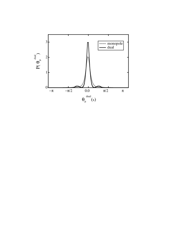
Figure 6.6: The comparison of the probability distribution $P(\theta_{\mu}^{\rm dual})$ with $P(\theta_{\mu}^{\rm Mo})$ in the monopole sector in the MA gauge. The dual gauge variable $\theta^{\rm dual}_{\mu}$ is defined in the dual Landau gauge $\partial_{\mu}\theta^{\rm dual}_{\mu}=0$. The angle variable $\theta_{\mu}^{\rm Mo}$ in the monopole sector satisfies the Landau gauge condition $\partial_{\mu}\theta_{\mu}^{\rm Mo}=0$.

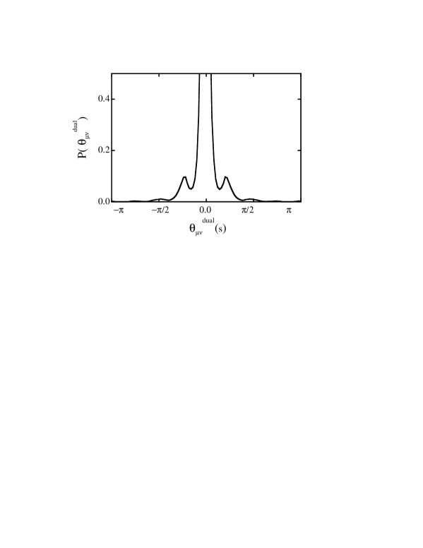
Figure 6.7: The probability distribution $P(\bar{\theta}_{\mu\nu}^{\rm dual})$ of the dual abelian field-strength $\bar{\theta}_{\mu\nu}^{\rm dual}$ in the monopole sector in the MA gauge. Here, $P(\bar{\theta}_{\mu\nu}^{\rm dual})$ exactly coincides with $P(\bar{\theta}_{\mu\nu}^{\rm Mo})$.

In Fig.6.6, we compare the probability distribution $P(\theta_{\mu}^{\rm dual})$ of dual gauge variable $\theta_{\mu}^{\rm dual}$ and $P(\theta_{\mu}^{\rm Mo})$ of the gauge variable $\theta_{\mu}^{\rm Mo}$ in the monopole sector in the MA gauge. Here, $\theta^{\rm dual}_{\mu}$ is defined in the dual Landau gauge $\partial_{\mu}\theta_{\mu}^{\rm dual}=0$, and $\theta^{\rm Mo}_{\mu}$ is defined in Eq.(6.1) satisfies the Landau gauge $\partial_{\mu}\theta_{\mu}^{\rm Mo}=0$. These two distributions seem to have almost the same widths. This is because the Dirac sheet $n_{\mu\nu}$ is strongly suppressed in the Landau gauge, while there is no dual Dirac sheets with $n_{\mu\nu}^{\rm dual}\neq 0$ in the dual Landau gauge owing to the absence of $j_{\mu}$. In fact, only the essential minimal fluctuation remains both for the monopole variable $\theta_{\mu}^{\rm Mo}$ in the Landau gauge and for the dual variable $\theta_{\mu}^{\rm dual}$ in the dual Landau gauge. Different from $\theta_{\mu}^{\rm Mo}$, however, $\theta_{\mu}^{\rm dual}$ has two bumps around $\theta_{\mu}^{\rm dual}=\pm\frac{\pi}{4}$ originated from the monopole current.

We show in Fig.6.7 the probability distribution $P(\bar{\theta}_{\mu\nu}^{\rm dual})$ of the dual abelian field-strength $\bar{\theta}_{\mu\nu}^{\rm dual}$. There appear also some bumps originated from the quantization of the monopole current and lattice discretization. Here, $P(\bar{\theta}_{\mu\nu}^{\rm dual})$ is the same as $P(\bar{\theta}_{\mu\nu}^{\rm Mo})$ because of $\bar{\theta}^{\rm dual}_{\mu\nu}={}^{*}\bar{\theta}^{\rm Mo}_{\mu\nu}$ in the continuum limit. However, the two-forms $\theta_{\mu\nu}^{\rm dual}\equiv(\partial\wedge\theta^{\rm dual})_{\mu\nu}$ differs from ${}^{*}\theta_{\mu\nu}^{\rm Mo}\equiv^{*}(\partial\wedge\theta^{\rm Mo})_{\mu\nu}$ according to the difference between $n_{\mu\nu}^{\rm dual}$ and ${}^{*}n_{\mu\nu}^{\rm Mo}$. In the description by $\theta^{\rm Mo}_{\mu\nu}$, there inevitably appears the singularity as the Dirac sheet with $n_{\mu\nu}\neq 0$ to generate the monopole current through the breaking of the Bianchi identity, although the appearance of the Dirac sheet is strongly suppressed in the Landau gauge. In the dual formalism, on the other hand, the monopole sector becomes regular and does not include the dual Dirac sheet, i.e. $n_{\mu\nu}^{\rm dual}=0$, in the dual Landau gauge owing to the dual Bianchi identity. Actually in the monopole sector in the dual Landau gauge, $\theta_{\mu\nu}^{\rm dual}\equiv(\partial\wedge\theta^{\rm dual})_{\mu\nu}$ distributes only in the region of $-\pi<\theta^{\rm dual}_{\mu\nu}<\pi$, and hence one fines $\bar{\theta}^{\rm dual}_{\mu\nu}\equiv\mbox{mod}_{2\pi}(\partial\wedge\theta^{\rm dual})_{\mu\nu}=\theta^{\rm dual}_{\mu\nu}$ and $n_{\mu\nu}^{\rm dual}=0$ everywhere on the lattice. Thus, the monopole sector in the lattice QCD is described by the dual gauge field without the singularity as the Dirac string in the dual Landau gauge.

Using the dual gauge variable $\theta_{\mu}^{\rm dual}$, the static potential between the monopole and the anti-monopole is obtained from the dual Wilson loop ${\rm tr}\prod_{i=1}^{\rm L}u_{\mu_{i}}^{\rm dual}(s_{i})$ with $u_{\mu}^{\rm dual}(s)\equiv{\rm exp}\{i\tau_{3}\theta_{\mu}^{\rm dual}(s)\}$ [57]. The large dual Wilson loop obeys the perimeter law, and the inter-monopole potential can be fitted by the Yukawa potential including the monopole size effect [57]. Thus, the dual gauge field $B_{\mu}$ seems to acquire its mass in the infrared region, which would be a direct evidence on the dual Higgs mechanism by monopole condensation occurring in the QCD vacuum.

6.4 Scaling Properties on Monopole Current and Dirac Sheet

In this section, we study the $\beta$-dependence of the gluon field and the field strength in the abelian, monopole and photon sectors in the MA gauge with the U(1)₃ Landau gauge. We study also the monopole-current density $\rho_{\rm MC}$ and the Dirac-sheet density $\rho_{\rm DS}$ using the lattice QCD simulation with various $\beta$. We argue these quantities both in the lattice unit and in the physical unit, and examine their scaling property.

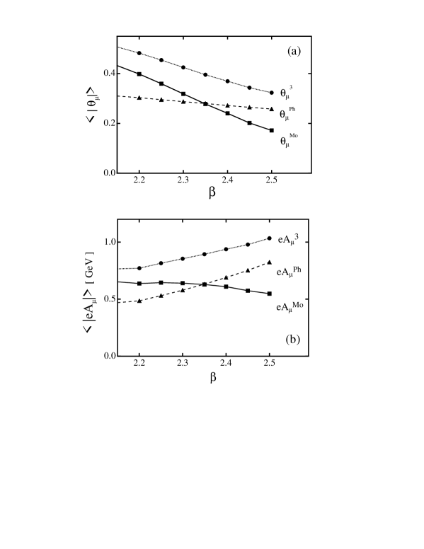
Figure 6.8: (a) The absolute value of the lattice angle variables $\theta^{3}_{\mu}(s)$, $\theta^{\rm Mo}_{\mu}(s)$, $\theta^{\rm Ph}_{\mu}(s)$ in the MA gauge with U(1)₃ Landau gauge fixing on $16^{4}$ lattice as the function of $\beta$. The solid, dotted and dashed lines denote $|\theta^{3}_{\mu}(s)|$, $|\theta^{\rm Mo}_{\mu}(s)|$ and $|\theta^{\rm Ph}_{\mu}(s)|$, respectively. (b) The absolute value of the continuum abelian gauge fields $|eA^{3}_{\mu}|$, $|eA^{\rm Mo}_{\mu}|$ and $|eA^{\rm Ph}_{\mu}|$ in the MA gauge on $16^{4}$ lattice as the function of $\beta$. These are obtained from $\theta_{\mu}\equiv A_{\mu}\cdot\frac{ae}{2}$ with lattice spacing $a$. The lattice spacing $a$ is defined so as to produce the string tension $\sigma=$0.89 GeV/fm.

In the MA gauge with the U(1)₃ Landau gauge, the probability distribution of abelian angle variables, $\theta_{\mu}^{3}$, $\theta_{\mu}^{\rm Mo}$ and $\theta_{\mu}^{\rm Ph}$, also exhibit a peak around $\theta_{\mu}=0$ as was shown in Fig.6.2. We show in Fig.6.8(a) the $\beta$-dependence of $\langle|\theta_{\mu}^{3}|\rangle$, $\langle|\theta_{\mu}^{\rm Ph}|\rangle$ and $\langle|\theta_{\mu}^{\rm Mo}|\rangle$ in the MA gauge with the U(1)₃ Landau gauge, and find that the fluctuation of the abelian angle variables decreases with $\beta$ on the average. On the continuum abelian fields, $eA_{\mu}\equiv\frac{2}{a}\theta_{\mu}^{3}$, $eA_{\mu}^{\rm Ph}\equiv\frac{2}{a}\theta^{\rm Ph}_{\mu}$ and $eA_{\mu}^{\rm Mo}\equiv\frac{2}{a}\theta^{\rm Mo}_{\mu}$, we show in Fig.6.8(b) the $\beta$-dependence on $\langle|eA_{\mu}|\rangle$, $\langle|eA_{\mu}^{\rm Ph}|\rangle$ and $\langle|eA_{\mu}^{\rm Mo}|\rangle$. While there appears a $\beta$-dependence on $eA_{\mu}$ and $eA_{\mu}^{\rm Ph}$, the continuum field $eA_{\mu}^{\rm Mo}$ in the monopole sector is also found to be less $\beta$-independent.

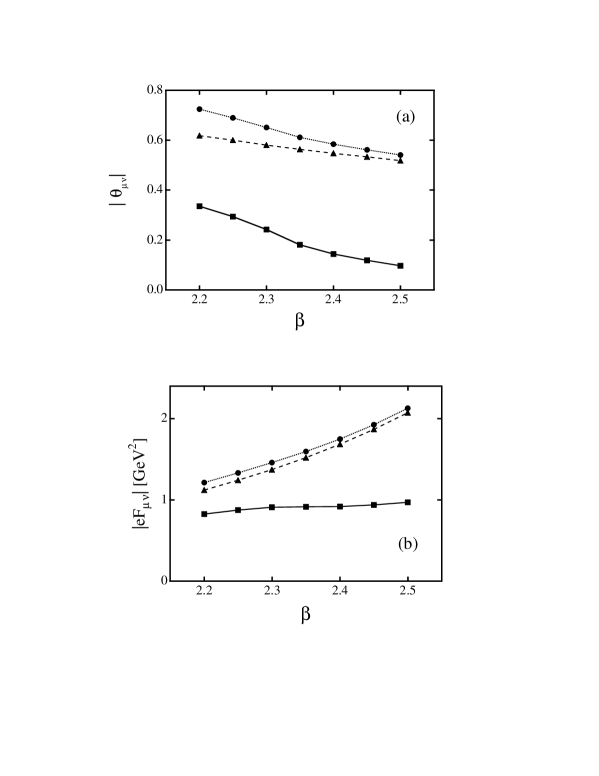
Figure 6.9: (a) The absolute value of the abelian field strength $|\bar{\theta}_{\mu\nu}|$ in the MA gauge as the function of $\beta$. The circle, square and triangle denote $|\bar{\theta}_{\mu\nu}|$ in the abelian, monopole and photon sectors, respectively. (b) The absolute value of the continuum abelian field strength $|eF_{\mu\nu}|\equiv|\bar{\theta}_{\mu\nu}|\cdot\frac{2}{a^{2}}$ in the physical scale as the function of $\beta$. The circle, square and triangle denote $|eF_{\mu\nu}|$ in the abelian, monopole and photon sectors, respectively.

In the MA gauge, the probability distribution of the abelian plaquette variable $\bar{\theta}_{\mu\nu}$, has a peak around $\bar{\theta}_{\mu\nu}=0$ as was shown in Fig.3.11, and hence the abelian plaquette action seems to control the abelian system like the SU(2) total action. Such a tendency on the gathering around $\bar{\theta}_{\mu\nu}=0$ becomes clearer as $\beta$ increases. Quantitatively, we show in Fig.6.9(a) the $\beta$-dependence of $\langle|\bar{\theta}_{\mu\nu}|\rangle$, $\langle|\bar{\theta}_{\mu\nu}^{\rm Ph}|\rangle$ and $\langle|\bar{\theta}_{\mu\nu}^{\rm Mo}|\rangle$ in the MA gauge, and find decreasing of all the plaquette angles with $\beta$. From these lattice data, we try to extract the continuum abelian field strength, $eF_{\mu\nu}\equiv\frac{2}{a^{2}}\bar{\theta}_{\mu\nu}$, $eF_{\mu\nu}^{\rm Ph}\equiv\frac{2}{a^{2}}\bar{\theta}^{\rm Ph}_{\mu\nu}$ and $eF_{\mu\nu}^{\rm Mo}\equiv\frac{2}{a^{2}}\bar{\theta}^{\rm Mo}_{\mu\nu}$. We show the $\beta$-dependence on $\langle|eF_{\mu\nu}|\rangle$, $\langle|eF_{\mu\nu}^{\rm Ph}|\rangle$ and $\langle|eF_{\mu\nu}^{\rm Mo}|\rangle$ in Fig.6.9(b), where the lattice constant $a$ used is determined so as to reproduce the string tension $\sigma$=0.89GeV/fm in the SU(2) sector. While there appears a $\beta$-dependence on $eF_{\mu\nu}$ and $eF_{\mu\nu}^{\rm Ph}$, the continuum field $eF_{\mu\nu}^{\rm Mo}$ in the monopole sector is almost $\beta$-independent. In other words, we find a good scaling property even for the local variable as $eF_{\mu\nu}^{\rm Mo}$ in the monopole sector.

In order to understand the good scaling property on the abelian continuum variables in the monopole sector, we examine the $\beta$-dependence of the monopole-current density $\rho_{\rm MC}$ and the Dirac-sheet density $\rho_{\rm DS}$ in the MA gauge with the U(1)₃ Landau gauge. In the physical unit, the monopole-current density $\rho_{\rm MC}$ is expressed as the ratio of the total monopole-current length $L_{\rm tot}^{phys}$ to 4-dimensional physical volume $V_{\rm tot}^{phys}$ of the system,

$$\rho_{\rm MC}^{phys}\equiv\frac{\rho_{\rm MC}^{lat}}{a^{3}}={\displaystyle\sum_{s,\mu}a|k_{\mu}(s)|\over\displaystyle\sum_{s,\mu}a^{4}}={L_{\rm tot}^{phys}\over V_{\rm tot}^{phys}}.$$ (6.20)

Similarly, the Dirac-sheet density $\rho_{\rm DS}$ in the physical unit is expressed as the ratio of the total Dirac-sheet area $S_{\rm tot}^{phys}$ to 4-dimensional physical volume $V_{\rm tot}^{phys}$ of the system,

$$\rho_{\rm DS}^{phys}\equiv\frac{\rho_{\rm DS}^{lat}}{a^{2}}={\displaystyle\sum_{s,\mu,\nu}a^{2}|n_{\mu\nu}(s)|\over\displaystyle\sum_{s,\mu,\nu}a^{4}}={S_{\rm tot}^{phys}\over V_{\rm tot}^{phys}}.$$ (6.21)

If the monopole-current length $L_{\rm tot}^{phys}$ and the Dirac-sheet area $S_{\rm tot}^{phys}$ are physical values in the continuum limit, $\rho_{\rm MC}^{phys}$ and $\rho_{\rm DS}^{phys}$ are to be almost $\beta$-independent as long as the mesh $a$ is small enough. We show in Fig.6.10 the $\beta$-dependence of $\rho_{\rm MC}^{phys}$ and $\rho_{\rm DS}^{phys}$ in the MA gauge with the U(1)₃ Landau gauge. As for the monopole density $\rho_{\rm MC}^{phys}$, there is a $\beta$-dependence to some extent. On the other hand, the Dirac-sheet density $\rho_{\rm DS}^{phys}$ is almost $\beta$-independent, and exhibit a clear scaling property.

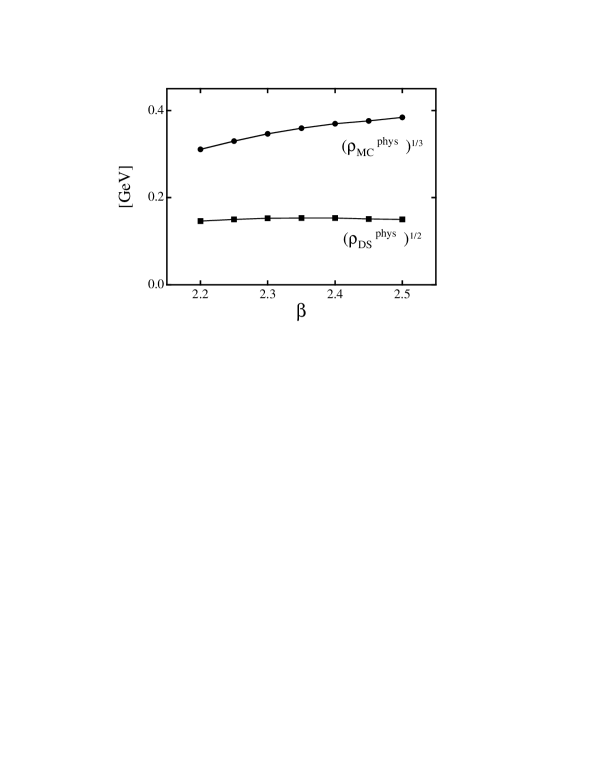
Figure 6.10: The monopole-current density $(\rho^{phys}_{\rm MC})^{\frac{1}{3}}$ and the Dirac-sheet density $(\rho_{\rm DS}^{phys})^{\frac{1}{2}}$ as the function of $\beta$ in the MA gauge on $16^{4}$ lattice. The area of the Dirac sheets is $\beta$-independent, while the monopole-current length slightly increases with $\beta$.

Thus, $n_{\mu\nu}^{phys}(s)\equiv n_{\mu\nu}(s)/a^{2}$ is expected to be almost $\beta$-independent on the average over the whole system. Near the continuum limit, we can then expect $a$-independence of $eA_{\mu}^{\rm Mo}$ as

$$eA_{\mu}^{\rm Mo}(s)=\frac{2}{a}\theta_{\mu}(s)^{\rm Mo}=\frac{2}{a}\sum_{s^{\prime}}D^{lat}(s-s^{\prime})\partial_{\alpha}^{lat}n_{\alpha\mu}(s^{\prime})\simeq\int d^{4}x^{\prime}D(s-x^{\prime})\partial_{\alpha}n_{\alpha\mu}^{phys}(x^{\prime}),$$

where the last expression is to be $a$-independent. Thus, the good scaling property of the Dirac-sheet density is considered as the origin of the approximate $\beta$-independence of the abelian continuum variables $eA_{\mu}^{\rm Mo}$ and $eF_{\mu\nu}^{\rm Mo}$ in the monopole sector.

It is noted that the Dirac-sheet area $S_{\rm tot}^{phys}$ seems to have a continuum limit in a fixed 4-dimensional physical volume $V_{\rm tot}^{phys}$, although the monopole-current length $L_{\rm tot}^{phys}$ tends to increase as the mesh $a$ decreases. Here, let us consider the reason of the good scaling for the Dirac-sheet area in the U(1)₃ Landau gauge. In the U(1)₃ Landau gauge, the U(1)₃ gauge variable $\theta^{3}_{\mu}(s)$ is forced to be mostly continuous as $\theta^{3}_{\mu}\simeq 0$ on the lattice, which suppresses the large $\theta_{\mu\nu}$ fluctuation which generates $n_{\mu\nu}\neq 0$ as was shown in Fig.3.10. Thus, the generation of the Dirac sheet is strongly suppressed in the U(1)₃ Landau gauge, although the Dirac sheet induced by the monopole current must appear. Geometrically, the area of the Dirac sheet is minimized in the U(1)₃ Landau gauge, within the constraint that the boundary of the Dirac sheet is fixed as the monopole current. This situation resembles the “soap bubble” with the boundary fixed. Thus, the Dirac-sheet area is insensitive to the small fluctuation of its boundary or the monopole current due to the minimizing condition of the area in the U(1)₃ Landau gauge.

On the lattice, as the mesh $a$ becomes small, the monopole current may be fractal, and the length of the monopole current may become large with small $a$. Nevertheless, the Dirac-sheet area remains almost unchanged in the U(1)₃ Landau gauge owing to the minimizing condition of the area, even when its boundary or the monopole current becomes fractal. This would be the advanced point of the use of the Dirac sheet in the U(1)₃ Landau gauge for the scaling property rather than the monopole current.

6.5 Estimation of the Wilson Loop from the Monopole

Up to now, we have found that the monopoles appearing in the MA gauge brings the large fluctuation of the abelian field variable around them, which would be the origin of the string tension. In this section, we consider the relation between the monopole density $\rho_{\rm Mo}$ and the string tension $\sigma$ in order to clarify the role of monopole for the confinement force in the analytical manner. Here, we idealizes the large field fluctuation created by the monopole, and pay attention to the area-law reduction of the Wilson loop $\langle W\rangle$. For the system with the monopole density $\rho_{\rm Mo}$, one (anti-) monopole is expected to occupy the area of the cube with the length $d_{\rm Mo}\equiv\rho_{\rm Mo}^{-1/3}$, which would be a typical scale of the confinement physics [58]. Here, $r_{\rm Mo}\equiv\frac{d_{\rm Mo}}{2}$ corresponds to the size of the QCD monopole, and is estimated as $r_{\rm Mo}\equiv 0.25\sim 0.3$fm from the lattice QCD with $\beta=2.4$ as shown in Fig.6.1. As an important feature, the unit-charge monopole provides a minus factor to the Wilson. Let us consider the static monopole with the unite charge and the “spatial” Wilson loop surrounding the monopole as shown in Fig.6.11 (a). Taking the plane sheet $S$ as the surface area inside the loop, one can use the simple estimation of the monopole effect as a “minus factor”,

$${\rm exp}\{ie\oint ds_{\mu}A_{\mu}^{3}\frac{\tau^{3}}{2}\}={\rm exp}\{ie\!\int\!\!\!\int\!\!d\sigma_{\mu\nu}F_{\mu\nu}^{3}\frac{\tau_{3}}{2}\}={\rm exp}\{i2\pi\!\!\times\!\!\frac{\tau^{3}}{2}\}={\rm exp}\{i\pi\tau^{3}\}=-1,$$

which corresponds to the half of the quantized magnetic flux between the monopole and anti-monopole as shown in Fig.6.11(b). In general, unit-charge monopole current which perpendicularly penetrates to the Wilson loop $W$ provides the “minus factor” to $W$.

Figure 6.11: (a) The monopole in the plaquette. In the lattice unite, the magnetic field surrounding the monopole is $\theta^{\rm total}_{\mu\nu}=2\pi$, and therefore the magnetic field penetrating the north or south half sphere is $\theta_{\mu\nu}=\pi$. The contribution of the monopole to the Wilson loop is $e^{ia^{2}ef_{\mu\nu}\frac{\tau_{3}}{2}}=e^{i\theta_{\mu\nu}\tau_{3}}=e^{i\pi\tau_{3}}=-1$. (b) The magnetic flux, which has positive and negative charges at the ends, penetrated in the plaquette. The quantization condition of the flux requires to $\theta_{\mu\nu}=2\pi n$ with $n\in{\bf Z}$. The contribution of this flux to the Wilson loop is $e^{ia^{2}ef_{\mu\nu}\frac{\tau_{3}}{2}}=e^{i\theta_{\mu\nu}\tau_{3}}=e^{i2\pi n\tau_{3}}=1$.

On the other hand, the effect of a monopole apart from the Wilson loop is expected largely canceled by the nearest anti-monopole, and is not expected to provide a large contribution to the Wilson loop in the dense monopole system like the AP-QCD vacuum. Such a screening effect is also suggested by recent lattice simulations on the inter-monopole potential [57]. Here, we try to estimate the contribution of monopoles to the Wilson loop of the $R\times T$ rectangular, where $R$ and $T$ are physical lengths. Defining the plane area $S$ inside the loop, we expect that only nearest monopoles to $S$ can contribute to the Wilson loop without the screening effect by other monopoles. Then, only monopoles inside $R\times T\times d_{\rm Mo}$ plate area near $S$ are provided the minus factor to the Wilson loop. The total monopole number in the $R\times T\times d_{\rm Mo}$ plate area is estimated as

$$N_{\rm Mo}\equiv(R\times T\times d_{\rm Mo})\times\rho_{\rm Mo}=\frac{R\times T}{d_{\rm Mo}^{2}}.$$ (6.22)

Introducing the lattice with a fine mesh $a\ll d_{\rm Mo}$, we try to estimate the Wilson loop as the function of $d_{\rm Mo}$. Since the lattice plaquette number on $S$ is $N^{lat}\equiv\frac{R\times T}{a^{2}}$, we divide the plate area $V$ into $N^{lat}$ “cells” as $a\times a\times d_{\rm Mo}$ boxes. When $a$ is taken small enough, each cell includes at most one (anti-)monopole, and the existence probability $q$ of the monopole inside one cell is obtained by $q=\frac{N_{\rm Mo}}{N^{lat}}=\frac{a^{2}}{d^{2}_{\rm Mo}}\ll 1$. Next, we apply the statistical consideration for the estimation of the Wilson loop $\langle W\rangle$. The probability that $n$ cells include the monopole among $N^{lat}$ cells is simply given ${}_{N^{lat}}C_{n}q^{n}(1-q)^{N^{lat}-n}$ in a statistical source. Since $n$ monopoles provide $(-)^{n}$ factor to the Wilson loop $W$, the expectation value $\langle W\rangle$ is estimated as

$$\langle W\rangle = \frac{\displaystyle\sum_{n=0}^{N^{lat}}{}_{N^{lat}}C_{n}q^{n}(1-q)^{N^{lat}-n}\times(-)^{n}}{\displaystyle\sum_{n=0}^{N^{lat}}{}_{N^{lat}}C_{n}q^{n}(1-q)^{N^{lat}-n}}=(1-2q)^{N^{lat}}$$ (6.23)

$$= {\rm exp}\{N^{lat}{\rm ln}(1-2q)\}={\rm exp}\{{\frac{R\times T}{a^{2}}{\rm ln}(1-2q)}\}.$$

Therefore, the Wilson loop obeys the area law, and the string tension $\sigma$ is obtained as

$$\sigma = -\frac{1}{R\times T}{\rm ln}\langle W\rangle=-\frac{1}{a^{2}}{\rm ln}(1-2q)=-\frac{1}{a^{2}}{\rm ln}(1-2\frac{a^{2}}{d_{\rm Mo}^{2}})\simeq\frac{2}{d_{\rm Mo}^{2}},$$ (6.24)

because of $q=\frac{a^{2}}{d_{\rm Mo}^{2}}\ll 1$. Thus, we derive a simple relation between the string tension $\sigma$ and the inter-monopole distance $d_{\rm Mo}$,

$$\sqrt{\sigma}\simeq\sqrt{2}\>d^{-1}_{\rm Mo}.$$ (6.25)

As shown in Fig.6.10, we have found $d_{\rm Mo}\equiv\rho^{-1/3}_{\rm Mo}=$ 0.5 $\sim$ 0.6 fm from the lattice result with $\beta=2.2\sim 2.5.$ Then, the string tension is evaluated as $\sqrt{\sigma}\simeq\sqrt{2}d^{-1}_{\rm Mo}=(0.42\simeq 0.57)$ GeV from the monopole density $\rho$ using this estimation.

Chapter 7 Monopole Current Dynamics

In the infrared region, color confinement can be understood by the dual Higgs theory with monopole condensation. The string tension is almost reproduced by the monopole sector of the abelian gluon component, which is called as monopole dominance for the color confinement force. Thus, the monopole degrees of freedom would be the key variable for the confinement physics. In the dual Higgs theory, the monopole is assumed to be condensed, which has been suggested by the formation of global network of the monopole current in the lattice QCD. In this chapter, we examine the realization of monopole condensation in the QCD-vacuum at the infrared scale. However, QCD is described by the gluon field not by the monopole current, and therefore it is difficult to clarify monopole condensation only with the lattice QCD simulation. To this end, we generate the monopole-current system on the lattice using a simple monopole current action and study the role of the monopole current to the color confinement[59]. Comparing the QCD vacuum with the monopole current system, we try to clarify the monopole condensation occurred in the non-perturbative QCD.

7.1 Monopole Current Dynamics and Kosterlitz-Thouless-type Transition

To begin with, we consider the monopole-current action $S[k_{\mu}(s)]$ which simulates the monopole-current system observed in the lattice QCD in the MA gauge. In general, $S[k_{\mu}(s)]$ includes the nonlocal Coulomb interaction as $S_{C}=\int d^{4}xd^{4}yk_{\mu}(x)D(x-y)k_{\mu}(y)$ with the Coulomb propagator $D(x)$. In the dual Higgs phase, however, the effective interaction between the monopole currents would be short-range due to the screening effect by the dual Higgs mechanism [20, 57] similar to the Debye screening [60]. Then, the partition functional of the monopole current $k_{\mu}(x)\equiv k_{\mu}^{3}(x)\cdot\tau^{3}/2$ would be written as

$$Z=\int{\it D}k_{\mu}{\rm exp}\{-\alpha\int_{a}d^{4}x{\rm tr}k^{2}_{\mu}(x)\}\delta(\partial^{\mu}k_{\mu}),$$ (7.1)

where $\alpha$ is the energy per unit length of the monopole current. Here, the $\delta$-function is necessary to ensure the current conservation $\partial^{\mu}k_{\mu}=0$, and $a$ is an ultraviolet cutoff larger than the screening length. To perform the path-integral (7.1), we put the system on the 4-dimensional lattice with the lattice spacing $a$. In the lattice formalism, the monopole currents are defined on the dual lattice,

$$k^{lat}_{\mu}(s)\equiv e/(4\pi)\cdot a^{3}k^{3}_{\mu}(s).$$ (7.2)

The partition function is given as

$$Z=\sum_{k^{lat}_{\mu}}{\rm exp}\{-\alpha^{lat}\sum_{s}k_{\mu}^{lat}(s)^{2}\}\delta(\partial_{\mu}k_{\mu}^{lat}(s)),$$ (7.3)

where $\alpha^{lat}\equiv\alpha/2\cdot(4\pi/ea)^{2}$.

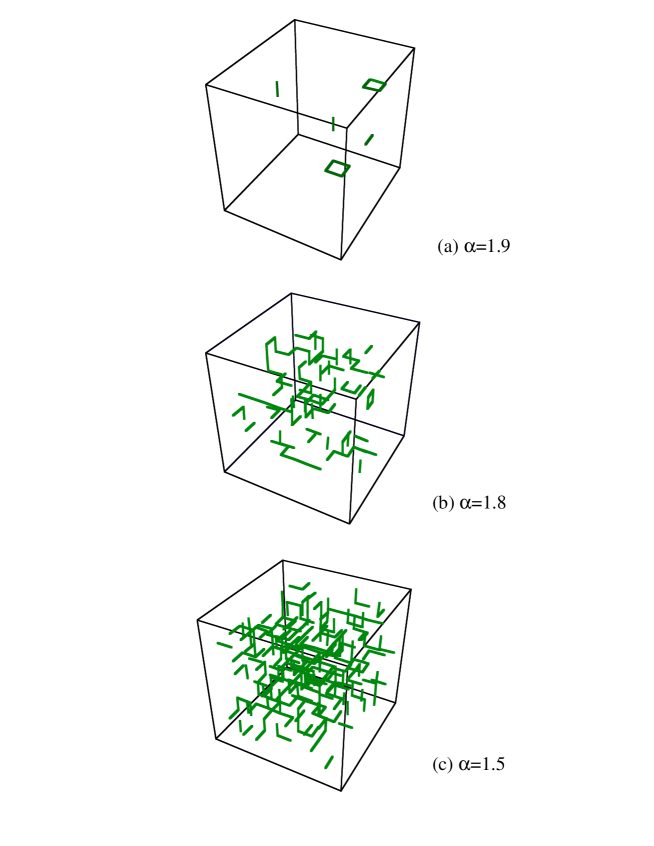
Figure 7.1: The monopole current in the monopole-current system in ${\bf R}^{3}$ at a fixed time : (a) the “critical phase” ($\alpha=1.9\simeq\ln 7$), (b) the “monopole condensed phase” near the critical point ($\alpha=1.8$) and (c) the “monopole condensed phase” ($\alpha=1.5$).

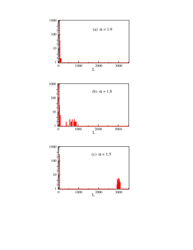
Figure 7.2: The histograms of the monopole-current length $L$ of each monopole cluster in the monopole-current system. The data at each $\alpha$ are taken from 40 current configurations. (a) In the “critical phase”, only short monopole loops appear. (b) In the “ monopole condensed phase” near the critical point, monopole currents become in a cluster. (c) In the “confinement phase”, there appears one large monopole cluster in each current configuration.

The lattice QCD simulation shows that one long monopole loop and many short loops appear in the confinement phase [61]. Only the long loop becomes important for the properties of the QCD vacuum, while many short loops are originated from the fluctuation in the ultraviolet region and therefore can be neglected. In this system, the partition function can be approximated as the single monopole loop ensemble with the length $L$,

$$Z=\sum_{L}\rho(L)e^{-\alpha L},$$ (7.4)

where $L$ and $\rho(L)$ are length of the monopole loop and its configuration number, respectively. The monopole current with length $L$ is regarded as the $L$ step self-avoiding random walk, where $2D-1=7$ direction is possible in each step in the $D$ dimensional space-time. Therefore, $\rho(L)$ is roughly estimated as $(2D-1)^{L}=7^{L}$. Using this partition function, the expectation value of the monopole current length is found to be

$$\langle L\rangle=\frac{1}{Z}\sum_{L}\rho(L)Le^{-\alpha L}=\left\{\begin{array}[]{ll}\{\alpha-\ln(2D-1)\}^{-1}&\mbox{if $\alpha>\ln(2D-1)$}\\ \infty&\mbox{if $\alpha<\ln(2D-1)$}.\end{array}\right.$$ (7.5)

When the energy $\alpha$ is larger than the entropy $\ln(2D-1)$, the monopole loop length is finite. However, when $\alpha$ is smaller than the entropy, the monopole loop length becomes infinite, which corresponds to monopole condensation in the current representation [20]. Here, the critical value on monopole condensation $\alpha_{c}\simeq{\rm ln}(2D-1)\simeq{\rm ln}7=1.945$, which corresponds to the “entropy” of the self-avoiding random walk. Such a transition is quite similar to the Kosterlitz-Thouless type transition in (1+2)-dimensional superconductor [21], where vortex condensation plays an important role to the transition.

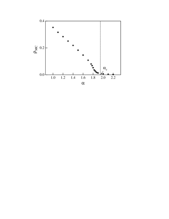
Figure 7.3: The monopole density $\rho_{MC}$ as the function of $\alpha$. The monopole density becomes small for large $\alpha$ and almost vanishes for $\alpha>\alpha_{c}={\rm ln}7=1.945$.

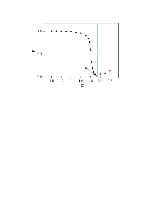
Figure 7.4: The clustering parameter $\eta\equiv\sum_{i}L_{i}^{2}/(\sum_{i}L_{i})^{2}$ as the function of $\alpha$. Near the critical point $\alpha_{c}=\ln 7=1.945$, $\eta$ is drastically changed from unity to zero.

In performing the simulation, we construct the monopole current as the sum of plaquettes of the monopole current because of the current conservation condition, $\partial_{\mu}k_{\mu}$ = 0. As the initial current configuration, we prepare a random monopole current system (hot start) or no monopole current system (cold start). Then, we update the link of the monopole current using the Metropolis method [42].

We generate the monopole current system using the monopole current action 7.3. Fig.7.1 shows the monopole current on $8^{4}$ lattices for the typical cases, ($\alpha=1.5,1.8,1.9$) at a fixed time. For these cases, we show in Fig.7.2 the histograms of monopole loop length [62] of each monopole cluster with 40 current configurations. For large $\alpha$, only small loops appear and monopole density is small. On the other hand, for small $\alpha$, there appears a global network of one large monopole cluster, and the monopole currents are complicated and dense. The lattice monopole density

$$\rho_{MC}\equiv\frac{1}{4V}\sum_{s,\mu}|k_{\mu}(s)|$$ (7.6)

and the clustering parameter

$$\eta\equiv\frac{\sum_{i}L^{2}_{i}}{(\sum_{i}L_{i})^{2}}$$ (7.7)

[63] are shown in Fig.7.3. and Fig.7.4, respectively. Here, $L_{i}$ is the loop length of the $i$-th monopole cluster. For the extreme limit of $\eta=1$, all the monopole loops are linked in a cluster, while many monopole loops are isolated for small $\eta$. As $\alpha$ decreases, the monopole density $\rho_{MC}$ becomes larger gradually for $\alpha\stackrel{{\scriptstyle<}}{{\scriptstyle{\sim}}}\alpha_{c}$. However, the clustering parameter is drastically changed at $\alpha=1.8$ closed to ${\rm ln7}$. Thus, these monopole current simulations clearly show the Kosterlitz-Thouless-type transition around $\alpha_{c}={\rm ln}7$ in agreement with the theoretical consideration on monopole (-current) condensation.

7.2 Role of Monopoles for Confinement

In this section, we study how these monopole currents contribute to the color confinement properties. Quark confinement is characterized by the linear inter-quark potential, which can be obtained from the area-law behavior of the Wilson loop, $\langle W\rangle=\langle P{\rm exp}({ie\oint A_{\mu}dx_{\mu}})\rangle$. Therefore, it is desired to extract the gauge variable from the monopole current $k_{\mu}$. We now derive the abelian gauge variable in stead of the non-abelian gauge field, because the lattice QCD results show that the color confinement phenomena can be discussed only with abelian part to some extent. However, in the presence of the magnetic monopoles, the ordinary abelian gauge field $A_{\mu}(x)$ inevitably includes the singularity as the Dirac string, which leads to some difficulties in the field theoretical treatment. Instead, the dual field formalism is much useful to describe the monopole current system, because the dual gauge field $B_{\mu}(x)$ can be introduced without the singularity for such a system with $k_{\mu}\neq 0$ and $j_{\mu}=0$. This is the dual version of the ordinary gauge theory with $A_{\mu}(x)$ for the QED system with $j_{\mu}\neq 0$ and $k_{\mu}=0$.

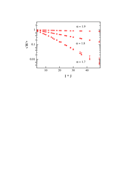
Figure 7.5: The expectation value of the Wilson loop $\langle W(I\times J)\rangle$ on the fine mesh $c=a/2$ for $\alpha=1.7,1.8,1.9$. The area-law behavior of $\langle W\rangle$ indicates the linear inter-quark potential, although the string tension is zero for $\alpha=1.9>\alpha_{c}$.

Now, we apply the dual field formalism to the monopole current system discussed in Section 7.1. Since the monopole current $k^{lat}_{\mu}(s)$ is generated on the lattice with the mesh $a$, the continuous dual field $B_{\mu}(x)$ is derived from $k_{\mu}(x)$ using Eq.(6.13), in principle. In estimating the integral in Eq.(6.13) numerically, we use a fine lattice with a small mesh $c$. To extract $B_{\mu}(x)$ correctly, the mesh $c$ is to be taken enough small. However, too fine mesh is not necessary because the original current $k^{lat}_{\mu}(s)$ includes the error in the order of $a$. Numerical analyses show that the use of $c\simeq a$ is too crude for the correct estimation of the integral in Eq.(6.13). Instead, the calculation with $c\leq a/2$ is good enough for the estimation of $B_{\mu}(x)$, and hence we take $c=a/2$ hereafter.

The expectation value of the Wilson loop $\langle W\rangle$ is shown in Fig.7.5. The Wilson loop exhibits the area-law and the linear confinement potential: ${\rm ln}\langle W\rangle$ decreases linearly with the inter-quark distance, where its slope corresponds to the string tension. Quantitatively, the string tension is measured by the Creutz ratio, and we show in Fig.7.6 $\chi(3,3)$ as a typical example.

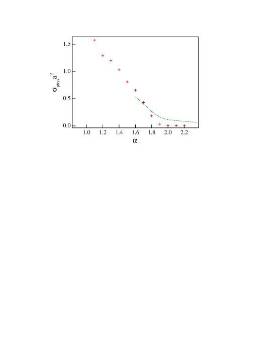
Figure 7.6: The Creutz ratio as the function of $\alpha$ in the monopole current system. The dotted line denotes the Creutz ratio as the function of $\beta=1.25\alpha$ in the lattice QCD.

For the monopole condensed phase as $\alpha<\alpha_{c}$, the string tension gets a finite value, while it vanishes for the non-condensed phase of monopole as $\alpha\leq\alpha_{c}$. Thus, the confinement phase directly corresponds to the monopole condensed phase and therefore monopole condensation is essential as essence of the confinement mechanism.

7.3 Monopole Condensation in the QCD Vacuum

In this section, we compare the lattice QCD with the monopole-current system in terms of monopole condensation and confinement properties, as shown in Fig.7.7. The lattice QCD simulation shows that the QCD vacuum in the MA gauge holds the global network of monopole current as shown in Section 4.3. Considering the similarity on the monopole clustering, the QCD vacuum can be regarded as the monopole-condensed phase with $\alpha<\alpha_{c}$ in the monopole current system, as shown in Fig.7.1(c). Such identification of the QCD vacuum with the monopole-condensed phase is also suggested in terms of the confinement properties, because the confinement phase corresponds to the monopole condensed phase as shown in Section 7.2.

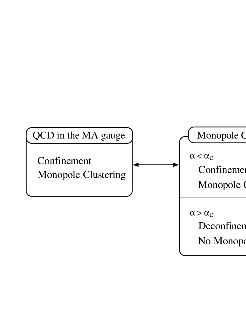
Figure 7.7: Comparison between QCD in the MA gauge and the monopole current system. The QCD vacuum corresponds to the monopole-condensed phase in the monopole current system because of the similarity on confinement and the monopole clustering.

7.4 Comparison with Vortex Condensation in 1+2 Superconductor

In this section, we summarize in Table 7.1 the correspondence between monopole condensation in the QCD vacuum and vortex condensation in the 1+2 dimensional superconductor [21] in terms of the topological object and the phase transition. For these two systems, condensation of the line-like topological object plays the relevant role for the determination of the phase. The phase structure is controlled by the balance of power between “entropy” (configuration number of the topological object) and “energy” (self-energy of the topological object).

In the 1+2 dimensional superconductor, the Abrikosov vortex is the important topological object. While the vortex scarcely appears at the low $T$, such topological excitations frequently occur at the high $T$, which enhances the entropy factor in the free energy. Then, at the critical temperature, vortex condensation occurs due to “entropy dominance” and the system goes to the normal phase. This phase transition is known as the Kosterlitz-Thouless transition.

Similarly in the QCD vacuum, the monopole current plays the relevant role as the line-like topological object in the 4-dimensional space-time. In the monopole-current system, the control parameter is the self-energy $\alpha$ of the monopole current. While only the local fluctuation of the monopole current appears for $\alpha>\alpha_{c}\simeq$ ln7, monopole condensation occurs for $\alpha<\alpha_{c}$ as the result of entropy dominance on the monopole-current configuration. Moreover, this monopole condensation leads to the electric confinement.

System	1+2 dim Superconductor	4-dim Monopole system
Line-like topological object	Vortex	Monopole current
Control parameter	Temperature $T$	Monopole self-energy $\alpha$
Condensed phase (Entropy dominance)	$High$ $temperature$ Normal phase $\uparrow$ Vortex condensation	$Small$ $\alpha$ Confinement phase $\uparrow$ Monopole condensation
Non-condensed phase (Energy dominance)	$Low$ $temperature$ Superconducting phase	$Large$ $\alpha$ Deconfinement phase

Table 7.1 Correspondence between the monopole current system and the 1+2 dimensional superconductor

7.5 Monopole Size and Critical Scale in QCD

Up to now, we have argued about the correspondence between the lattice QCD and the monopole current system described by (7.1) in terms of the qualitative aspects as monopole condensation and confinement. In the final section of this chapter, we attempt further consideration on the correspondence between the coupling constants, $\alpha$ and $\beta\equiv\frac{2N_{c}}{e^{2}}$. Here, we note also the limitation of the simple “monopole current approach” in the ultraviolet region and the critical scale of the dual superconductor picture of QCD.

To begin with, let us consider one magnetic monopole with an intrinsic radius $R$ in the multi-monopole system. In the static frame of the monopole, it creates a spherical magnetic field, ${\bf H}(r)={g(r)\over 4\pi r^{3}}{\bf r}={{\bf r}\over e(r)r^{3}}$ for $r\geq R$ and ${\bf H}(r)={g(r)\over 4\pi R^{3}}{\bf r}={{\bf r}\over e(r)R^{3}}$ for $r\leq R$, where the QCD running gauge coupling $e(r)$ is used to include the vacuum polarization effect. Here, the effective magnetic-charge distribution is assumed to be constant inside the monopole for the simplicity.

Now, we consider the lattice formalism with a large mesh $a>R$. The electromagnetic energy observed on the lattice around a monopole is roughly estimated as

$$M(a)\simeq\int_{a}^{\infty}d^{3}x{1\over 2}{\bf H}(r)^{2}\simeq{g^{2}(a)\over 8\pi a}={2\pi\over e^{2}(a)a},$$ (7.8)

which is largely changed depending on the lattice mesh $a$. This simple estimation neglects the possible reduction of $g(r)$ in the infrared region due to the asymptotic freedom of QCD. The screening effect of the magnetic field by other monopoles also reduces $g(r)$ effectively in a dense monopole system. However, $M(a)$ is modified by at most factor 2 ($M(a)=\frac{\pi}{e^{2}(a)a}$) even for the screening case as $g(r)=g(a)\cdot\theta(2a-r)$. Then, even in the multi-monopole system, $M(a)$ would provide an approximate value for the electromagnetic energy on lattices created by one monopole, and we call $M(a)$ as “lattice monopole mass”.

For the large mesh $a>R$, the monopole contribution to the lattice action reads $S=M(a)a\cdot L$, where $L$ denotes the length of the monopole current measured in the lattice unit $a$. Therefore, $M(a)$ is closely related to the monopole-current coupling $\alpha^{lat}$ and $\beta=2N_{c}/e^{2}$, $\alpha^{lat}\simeq M(a)a\simeq{2\pi\over e^{2}(a)}={\pi\over 2}\cdot\beta_{\rm SU(2)}.$ For the above screening case, this relation becomes $\alpha^{lat}\simeq M(a)a\simeq{\pi\over e^{2}(a)}={\pi\over 4}\cdot\beta_{\rm SU(2)},$ which is consistent with the numerical result, $\alpha=0.8\beta$, discussed in Section 7.2. Here, as long as the mesh is large as $a>R$, the lattice monopole action would not need modification by the monopole size effect, and the current coupling $\alpha^{lat}$ is proportional to $\beta$. Quantum mechanically, there is the energy fluctuation about $a^{-1}$ at the scale $a$, and therefore monopole excitation occurs very often at the long-distance scale satisfying $M(a)\stackrel{{\scriptstyle<}}{{\scriptstyle{\sim}}}a^{-1}$. Thus, $M(a)a\simeq\alpha^{lat}$ is the control parameter for monopole excitation at the scale $a(>R)$, and we can obtain the quantitative criterion for “monopole condensation” as $M(a)a\stackrel{{\scriptstyle<}}{{\scriptstyle{\sim}}}{\rm ln}(2D-1)$ from the analysis using the current dynamics in Section 7.1.

Second, we discuss the ultraviolet region with $a<R$. In the current dynamics, there exists a critical coupling $\alpha_{c}\simeq{\rm ln}(2D-1)$ as shown in Section 7.1 and 7.2. Above $\alpha_{c}$, the lattice current action provides no monopole condensation and no confinement, while $\beta\rightarrow\infty$ can be taken in the original QCD keeping the confinement property shown in Fig.7.6. Such a discrepancy between $\beta$ and $\alpha$ can be naturally interpreted by introducing the monopole size effect. Obviously, the monopole-current theory should be drastically changed in the ultraviolet region as $a<R$, if the QCD-monopole has its peculiar size $R$.

Here, let us reconsider the relation between $a$ and $\alpha^{lat}$ in the lattice current action. Similarly in the lattice QCD, the action has no definite scale except for the lattice mesh $a(>R)$, and therefore the scale unit $a$ would be determined so as to reproduce a suitable dimensional variable, e.g. the string tension $\sigma\simeq$ 1GeV/fm, in the monopole current dynamics. For instance, $a$ is determined as a function of $\alpha^{lat}$ using the Creutz ratio $\chi\simeq\sigma a^{2}$ in Fig.7.6. Therefore, $a$ should reach $R$ before realizing $\alpha^{lat}\rightarrow\alpha^{lat}_{c}$, and the framework of the current theory is to be largely modified due to the monopole size effect for $a<R$.

In conclusion, the QCD-monopole size $R$ provides a critical scale $R_{c}$ for the description of QCD in terms of the dual Higgs mechanism. Quantitatively, the difference between the monopole current system and QCD appear larger than $\beta=1.25\alpha$, which corresponds to $R_{c}\simeq 0.25$fm. In the infrared region as $a>R_{c}$, QCD can be approximated as a local monopole-current action [20], and the QCD vacuum can be regarded as the dual superconductor. On the other hand, in the ultraviolet region as $a<R_{c}$, the monopole theory becomes nonlocal and complicated due to the monopole size effect, and the perturbative QCD would be applicable instead.

Chapter 8 Dual Ginzburg-Landau Theory

The lattice QCD simulation shows abelian dominance and monopole dominance for the string tension in the maximally abelian (MA) gauge [23, 24, 26], and hence the monopole is considered to be the essential degrees of freedom for the confinement properties. In the confinement phase in the MA gauge, there appears the long and complicated monopole current covering the whole lattice space, which suggests monopole condensation. Thus, monopole condensation scheme is one of the realistic candidates of the physical interpretation for the confinement mechanism. In this chapter, we study the confinement phenomena using the dual Ginzburg-Landau (DGL) theory [22, 33], where the confinement mechanism is described by monopole condensation [15, 16, 17].

The DGL theory [22, 33] is the infrared effective theory of QCD based on the dual superconductor picture. In the ordinary Ginzburg-Landau theory, condensation of the Cooper-pair field leads to exclusion or squeezing of the magnetic field in the superconductor. Here, the U(1)_e-gauge symmetry is spontaneously broken and the abelian gauge field, the photon, becomes massive as the result of the Higgs mechanism. The Cooper-pair field plays a role of the Higgs field. In the QCD vacuum, condensation of the “monopole field” would provide the exclusion or squeezing of the color-electric field through the dual Meissner effect. In the monopole-condensed system, the dual gauge symmetry is spontaneously broken and the “dual gauge field” becomes massive.

Let us formulate the DGL theory starting from QCD. The QCD Lagrangian has the SU($N_{c}$) symmetry and is written by the quark field $q(x)$ and the gluon field $A_{\mu}(x)$ as

$${\cal L}_{\rm QCD}=-\frac{1}{2}{\rm tr}\left(G_{\mu\nu}G^{\mu\nu}\right)+\bar{q}\left(i\gamma_{\mu}D^{\mu}-m\right)q,$$ (8.1)

where $G_{\mu\nu}$ denotes the SU($N_{c}$) field strength,

$$G_{\mu\nu}\equiv\frac{1}{ie}([{\hat{D}_{\mu}},{\hat{D}_{\nu}}]-[\hat{\partial}_{\mu},\hat{\partial}_{\nu}])\hskip 28.45274pt\mbox{\rm with}\hskip 14.22636pt\hat{D}_{\mu}\equiv\hat{\partial}_{\mu}+ieA_{\mu}.$$ (8.2)

In terms of the Cartan decomposition, the gluon field $A_{\mu}(x)\equiv A_{\mu}^{a}(x)T^{a}$ $\in$ su($N_{c}$) with $N_{c}$=3 is decomposed into the diagonal component $\vec{A_{\mu}}=(A_{\mu}^{3},A_{\mu}^{8})$ and the off-diagonal component $C^{a}_{\mu}\in{\bf C}$,

$$A_{\mu}=\vec{A}_{\mu}\cdot\vec{H}+\sum\limits_{a=1}^{3}({C_{\mu}^{*a}}E_{a}+C_{\mu}^{a}E_{-a}).$$ (8.3)

Here, the Cartan subalgebra $\vec{H}$ is defined as

$${\vec{H}\equiv(H_{1},H_{2})\equiv(T_{3},T_{8}),}$$ (8.4)

and the raising and the lowering operators $E_{\pm a}(a=1,2,3)$ are defined as

$${E_{\pm 1}\equiv{1\over{\sqrt{2}}}(T_{1}\pm iT_{2})},\hskip 14.22636pt{E_{\pm 2}\equiv{1\over{\sqrt{2}}}(T_{4}\mp iT_{5})},\hskip 14.22636pt{E_{\pm 3}\equiv{1\over{\sqrt{2}}}(T_{6}\pm iT_{7})}.$$ (8.5)

One finds the relations $\left[{\vec{H},E_{a}}\right]=\vec{\alpha}_{a}E_{a}$ and $\left[{\vec{H},E_{-a}}\right]=-\vec{\alpha}_{a}E_{-a}$, where $\vec{\alpha}_{a}$ denotes the root vector of the SU(3) algebra: ${\vec{\alpha}_{1}=(1,0)}$, ${\vec{\alpha}_{2}=(-{1\over 2},-{{\sqrt{3}}\over 2})}$ and ${\vec{\alpha}_{3}=(-{1\over 2},{{\sqrt{3}}\over 2})}$. The off-diagonal gluon component $C_{\mu}^{a}$ is written as

$${C_{\mu}^{1}={1\over{\sqrt{2}}}(A_{\mu}^{1}+iA_{\mu}^{2})},\hskip 14.22636pt{C_{\mu}^{2}={1\over{\sqrt{2}}}(A_{\mu}^{4}-iA_{\mu}^{5})},\hskip 14.22636pt{C_{\mu}^{3}={1\over{\sqrt{2}}}(A_{\mu}^{6}+iA_{\mu}^{7})}.$$ (8.6)

According to the Cartan decomposition, the QCD Lagrangian is expressed as

$${\cal L}_{\rm QCD} = {\cal L}^{\rm Abel}+{\cal L}^{\rm off},$$ (8.7)

where ${\cal L}^{\rm Abel}$ is diagonal part of ${\cal L}_{\rm QCD}$,

$${\cal L}^{\rm Abel} = -\frac{1}{4}\left(\partial_{\mu}{\vec{A_{\nu}}}-\partial_{\nu}{\vec{A_{\mu}}}\right)^{2}{+\bar{q}(i\gamma_{\mu}\partial^{\mu}-e\gamma_{\mu}\vec{A}^{\mu}\cdot\vec{H}-m)q},$$ (8.8)

and ${\cal L}^{\rm off}$ is remaining part including the off-diagonal gluons,

$${\cal L}^{\rm off} = -{{1\over 2}\sum\limits_{a=1}^{3}{\left|{\left({(\partial_{\mu}-ie(\vec{\alpha}^{a}\cdot\vec{A}_{\mu}))\wedge C^{a}}\right)_{\mu\nu}-{{ie}\over{\sqrt{2}}}\alpha_{abc}C_{\mu}^{*b}C_{\nu}^{*c}}\right|}^{2}}$$ (8.9)

$${-{{ie}\over 2}\sum\limits_{a=1}^{3}{(\vec{f}_{\mu\nu}\cdot\vec{\alpha}_{a})}(C^{*a}\wedge C^{a})^{\mu\nu}}{+{e^{2}\over 4}\left[{\sum\limits_{a=1}^{3}{\vec{\alpha}_{a}(C^{*a}\wedge C^{a})_{\mu\nu}}}\right]^{2}}$$

$$-{e\sum\limits_{a=1}^{3}{\left[{C^{*a}_{\mu}(\bar{q}\gamma^{\mu}E_{a}q)+C^{a}_{\mu}(\bar{q}\gamma^{\mu}E_{-a}q)}\right]}}$$

with $(a\wedge b)_{\mu\nu}\equiv a_{\mu}b_{\nu}-b_{\mu}a_{\nu}$.

In the abelian gauge defined by diagonalizing a gauge dependent operator $\Phi$, the SU(3) gauge theory is reduced into [ U(1)₃ $\times$ U(1)₈]^e gluon gauge theory [22, 33] and monopoles appear. Particularly, in the MA gauge, off-diagonal components are forced to be small and behave as massive fields, while diagonal gluon components remain largely propagate over the long range [48]. In fact, in the MA gauge, off-diagonal gluons are infrared-irrelevant and can be neglected at the long distance. Therefore, after MA gauge fixing with $\Omega$, we construct the abelian projected QCD by dropping off the charged part and define the abelian gauge field ${\cal A}_{\mu}$ as

$${\cal A}_{\mu}\equiv\frac{1}{2}{\rm tr}(A_{\mu}\vec{H})\cdot\vec{H}\equiv\vec{A}_{\mu}\cdot\vec{H}.$$ (8.10)

Accordingly, the SU(3) field strength

$$G_{\mu\nu}^{\Omega}=(\partial_{\mu}A_{\nu}-\partial_{\nu}A_{\mu})+ie[A_{\mu},A_{\nu}]+\frac{i}{e}\Omega[\partial_{\mu},\partial_{\nu}]\Omega^{\dagger}$$ (8.11)

is modified as

$${\cal F}_{\mu\nu}=\partial_{\mu}{\cal A}_{\nu}-\partial_{\nu}{\cal A}_{\mu}-{\cal F}_{\mu\nu}^{\rm sing},$$ (8.12)

where ${\cal F}_{\mu\nu}^{\rm sing}=\frac{i}{e}\Omega[\partial_{\mu},\partial_{\nu}]\Omega^{\dagger}$. This corresponds to Eq.(4.24) in the lattice formalism. Here, the breaking of the abelian Bianchi identity is brought by the appearance of ${\cal F}_{\mu\nu}^{\rm sing}$. In the SU(3) case, there are three kinds of magnetic charges of the QCD-monopole corresponding to the subspace on degeneracy of the diagonalized operator $\Phi_{\rm diag}$; for $\Phi_{diag}={\rm diag}(\Phi_{1},\Phi_{2},\Phi_{3})$, $\Phi_{1}=\Phi_{2}$, $\Phi_{2}=\Phi_{3}$ and $\Phi_{3}=\Phi_{1}$. For example, the magnetic charge is proportional to the root vector $\vec{\alpha}_{1}$ in the case of the $\Phi_{1}=\Phi_{2}$. Thus, the magnetic charge of the monopole current is discretized as

$$\vec{m}=g\sum\limits_{a=1}^{3}\xi_{a}\vec{\alpha_{a}},\hskip 28.45274pt\xi_{a}\in{\bf Z}.$$ (8.13)

For $N$ monopole system, the magnetic current $k_{\mu}\equiv\vec{k}_{\mu}\cdot\vec{H}$ is expressed as

$$\vec{k}^{\mu}(x)=-g\sum\limits_{l=1}^{N}{\vec{m}_{l}\int{d\tau_{l}}}\frac{d\overline{x}_{l}^{\mu}(\tau_{l})}{d\tau_{l}}\delta^{4}(x-\bar{x}_{l}(\tau_{l})).$$ (8.14)

In the DGL theory, the monopole field is introduced by integrating over all trajectories of the monopole particle as will be shown in the later section.

8.1 Dual Gauge Field

The extended Maxwell equation is described by the field strength $F_{\mu\nu}$ as

$$\partial_{\nu}F^{\nu\mu}=j^{\mu},\hskip 56.9055pt\partial_{\nu}^{*}F^{\nu\mu}=k^{\mu}$$ (8.15)

with the electric current $j_{\mu}$ and the magnetic current $k_{\mu}$, and the electro-magnetic duality ($F_{\mu\nu}\leftrightarrow{}^{*}F_{\mu\nu}$, $j_{\mu}\leftrightarrow k_{\mu}$) is manifest in this formalism. In the ordinary QED, the description by the gauge field $A_{\mu}$ is useful, since QED includes only the electric current. In this description by $A_{\mu}$, however, this electro-magnetic duality in the Maxwell equation is not manifest and the introduction of the magnetic monopole leads to the singularity in the gauge field $A_{\mu}$. As shown in Section 6.3, for “the dual system” including only the magnetic current, it is rather useful to take the dual description with the dual gauge field $B_{\mu}$ instead of $A_{\mu}$. Here, the dual gauge field $B_{\mu}$ is introduced so as to satisfy

$${}^{*}F^{\mu\nu}=\frac{1}{2}\varepsilon^{\mu\nu\alpha\beta}F_{\alpha\beta}\equiv\partial^{\mu}B^{\nu}-\partial^{\nu}B^{\mu},$$ (8.16)

or equivalently, the electro-magnetic field is written as

$$E^{i} = \frac{1}{2}\varepsilon^{ijk}{}^{*}F^{jk}=\varepsilon^{ijk}\partial^{j}B^{k},$$ (8.17)

$$H^{i} = -^{*}F^{0i}=-\partial^{0}B^{i}+\partial^{i}B^{0}.$$ (8.18)

Now, we adopt here the Zwanziger formalism [64] described both with $A_{\mu}$ and $B_{\mu}$ in order to keep the electro-magnetic duality in the extended Maxwell equation manifest. In the general case with $j_{\mu}\neq 0$ and $k_{\mu}\neq 0$, we rewrite the field strength to keep the duality manifest in the following way. For an arbitrary anti-symmetric tensor $G_{\mu\nu}$ and an arbitrary constant four-vector $n_{\mu}$, there is an identity

$$G={1\over{n^{2}}}\left\{{\left[{n\wedge\left({n\cdot G}\right)}\right]-^{*}\left[{n\wedge\left({n\cdot^{*}G}\right)}\right]}\right\}$$ (8.19)

with $(n\cdot G)_{\mu}\equiv n_{\alpha}G^{\alpha\mu}$. Substituting $G=F=(\partial\wedge A)$ and ${}^{*}G={}^{*}F=(\partial\wedge B)$, we get

$$F = {1\over{n^{2}}}(\left\{{{n\wedge\left[{n\cdot(\partial\wedge A)}\right]}}\right\}-^{*}\left\{{n\wedge\left[{n\cdot(\partial\wedge B)}\right]}\right\}),$$ (8.20)

$${}^{*}F = {1\over{n^{2}}}({}^{*}\left\{{{n\wedge\left[{n\cdot(\partial\wedge A)}\right]}}\right\}+\left\{{n\wedge\left[{n\cdot(\partial\wedge B)}\right]}\right\}),$$ (8.21)

and then the extended Maxwell equations $\partial_{\nu}F^{\nu\mu}=j^{\mu}$ and $\partial_{\nu}^{*}F^{\nu\mu}=k^{\mu}$ are written as

$$\partial_{\nu}F^{\nu\mu} = {1\over{n^{2}}}\Bigl{(}\left\{{(n\cdot\partial)^{2}A^{\mu}-(n\cdot\partial)\partial^{\mu}(n\cdot A)-n^{\mu}(n\cdot\partial)(\partial\cdot A)+n^{\mu}\partial^{2}(n\cdot A)}\right\}$$

$$-{(n\cdot\partial)\varepsilon^{\mu}{}_{\nu\kappa\lambda}n^{\nu}\partial^{\kappa}B^{\lambda}}\Bigr{)}=j^{\mu},$$

$$\partial_{\nu}^{*}F^{\nu\mu} = {1\over{n^{2}}}\Bigl{(}\left\{{(n\cdot\partial)^{2}B^{\mu}-(n\cdot\partial)\partial^{\mu}(n\cdot B)-n^{\mu}(n\cdot\partial)(\partial\cdot B)+n^{\mu}\partial^{2}(n\cdot B)}\right\}$$

$$+{(n\cdot\partial)\varepsilon^{\mu}{}_{\nu\kappa\lambda}n^{\nu}\partial^{\kappa}A^{\lambda}}\Bigr{)}=k^{\mu}.$$

Therefore, the Lagrangian which leads to these field equations is derived as

$${\cal L} = -{1\over{2n^{2}}}\left[{n\cdot(\partial\wedge A)}\right]\left[{n\cdot^{*}(\partial\wedge B)}\right]+{1\over{2n^{2}}}\left[{n\cdot(\partial\wedge B)}\right]\left[{n\cdot^{*}(\partial\wedge A)}\right]$$ (8.22)

$$-{1\over{2n^{2}}}\left[{n\cdot(\partial\wedge A)}\right]^{2}-{1\over{2n^{2}}}\left[{n\cdot(\partial\wedge B)}\right]^{2}-j_{\mu}A^{\mu}-k_{\mu}B^{\mu}.$$

In the Zwanziger formalism, the duality transformation $F_{\mu\nu}\leftrightarrow{}^{*}F_{\mu\nu}$ is given by the replacement $A_{\mu}\leftrightarrow B_{\mu}$ and the electro-magnetic duality is manifest, and the system can be described without singularities. Particularly in the absence of $j_{\mu}$ and $k_{\mu}$, the theory can be written using “only $A_{\mu}$”, “only $B_{\mu}$”, or “both $A_{\mu}$ and $B_{\mu}$” in the Zwanziger formalism as

$$\int{{\cal D}Ae^{i\int{d^{4}x{\cal L}_{0}[A]}}}=\int{{\cal D}Be^{i\int{d^{4}x{\cal L}_{0}[B]}}}=\int{{\cal D}A{\cal D}Be^{i\int{d^{4}x{\cal L}_{0}[A,B]}}},$$ (8.23)

where

$${\cal L}_{0}[A] \equiv -{1\over 4}(\partial\wedge A)^{2},$$ (8.24)

$${\cal L}_{0}[A,B] \equiv -{1\over{2n^{2}}}\left[{n\cdot(\partial\wedge A)}\right]\left[{n\cdot^{*}(\partial\wedge B)}\right]+{1\over{2n^{2}}}\left[{n\cdot(\partial\wedge B)}\right]\left[{n\cdot^{*}(\partial\wedge A)}\right]$$ (8.25)

$$-{1\over{2n^{2}}}\left[{n\cdot(\partial\wedge A)}\right]^{2}-{1\over{2n^{2}}}\left[{n\cdot(\partial\wedge B)}\right]^{2},$$

$${\cal L}_{0}[B] \equiv -{1\over 4}(\partial\wedge B)^{2}.$$ (8.26)

In the Zwanziger formalism, the Lagrangian can be written with holding the duality between the gauge field $A_{\mu}$ and the dual gauge field $B_{\mu}$. However, occasionally it is more useful to describe only with $A_{\mu}$ or $B_{\mu}$ for practical calculations. Here, we try to describe the Lagrangian with only $A_{\mu}$ or $B_{\mu}$ by the functional integration over $B_{\mu}$ or $A_{\mu}$ in the partition functional [65].

Since the dual gauge field $B_{\mu}$ is bilinear in the Lagrangian (8.25), $B_{\mu}$ can be analytically integrated in the partition functional in the Zwanziger formalism,

$$\int{\cal D}A{\cal D}Be^{i\int d^{4}x{\cal L}[A,B]}=\int{\cal D}Ae^{i\int d^{4}x{\cal L}_{k}[A]}$$ (8.27)

with

$${\cal L}_{k}[A]=-{1\over 4}\{(\partial\wedge A)_{\mu\nu}-F^{\rm sing}_{\mu\nu}\}^{2}.$$ (8.28)

Here, the singular term $F_{\mu\nu}^{\rm sing}\equiv\varepsilon_{\mu\nu\alpha\beta}{1\over{n\cdot\partial}}n^{\alpha}k^{\beta}$ appears due to existence of the magnetic current $k_{\mu}$, and includes the nonlocal operator $\langle x|\frac{1}{n\cdot\partial}|y\rangle=\theta(x_{n}-y_{n})\delta^{3}(x_{\bot}-y_{\bot})$.

Thus, the field strength $F_{\mu\nu}$ includes the nonlocality in this description only by $A_{\mu}$ in the presence of the magnetic current $k_{\mu}$. Similarly, the theory can be described only with the dual gauge field $B_{\mu}$ after the functional integration on $A_{\mu}$. In this case, the theory is replaced by $(B_{\mu},j_{\mu})$ in the above argument, and the Lagrangian reads

$${\cal L}_{j}[B]=-{1\over 4}\{{}^{*}(\partial\wedge B)_{\mu\nu}-\varepsilon_{\mu\nu\alpha\beta}{1\over{n\cdot\partial}}n^{\alpha}j^{\beta}\}^{2},$$ (8.29)

where the nonlocal part appears ${}^{*}F_{\mu\nu}$ reflecting existence of the electric current $j_{\mu}$.

In this way, the system including both the electric and the monopole currents can be described without any singularities using the Zwanziger formalism, where the dual field $B_{\mu}$ is introduced as well as the gauge field $A_{\mu}$. On the other hand, the description only with $A_{\mu}$ or $B_{\mu}$ leads to the appearance of the nonlocal operator in the field strength in the general case. In constructing the DGL theory from abelian projected QCD, the above formalism can be applied by the simple replacement of $A_{\mu}\rightarrow{\cal A}_{\mu}\equiv\vec{A}_{\mu}\cdot\vec{H}$, $B_{\mu}\rightarrow{\cal B}_{\mu}\equiv\vec{B}_{\mu}\cdot\vec{H}$ and so on.

8.2 Monopole Field from the Monopole Particle

In this section, we derive the Lagrangian for the monopole field from the monopole-particle trajectories following Stone and Thomas [66, 67, 68]. At the infrared scale in the MA gauge, the monopole current becomes dense and complicated, and the monopole currents interact each other only in the short distance due to the screening effect [57] corresponding to monopole current. The infrared effective action $k_{\mu}$ is expected to be described by the local action of $k_{\mu}$

$$Z=\int_{a}dk_{\mu}e^{-\alpha k^{2}_{\mu}}.$$ (8.30)

Here, $\alpha$ is the monopole self-energy and the “mesh” $a$ is introduced as an ultraviolet cut-off larger than the screening length [59]. As shown Section 4.1, almost all monopoles have the unit charge in the abelian gauge, and therefore the partition functional is approximately described by the ensemble of the monopole loops

$$Z=\sum_{N}\frac{Z^{N}_{\rm loop}}{N!}\hskip 28.45274pt\mbox{with}\hskip 28.45274ptZ_{\rm loop}\equiv\sum_{L=0}^{\infty}\rho(L)e^{-\alpha L},$$ (8.31)

where $\rho(L)$ is the number of closed loop configurations with the length $L$. Here, we have taken the lattice unit $a=1$. Each monopole loop with the length $L$ can be approximated as $L$ step random walk [66] because of the absence of the nonlocal interaction.

Let us consider the grand canonical ensemble for closed-loops on the $D$-dimensional lattice in the unit of the lattice spacing 1. At the infrared scale, the partition function for a single monopole loop is written as

$$Z_{\rm loop}=\int_{0}^{\infty}d\tau\rho(\tau)e^{-\alpha\tau}.$$ (8.32)

The probability distribution of starting at $x$ and ending at $x^{\prime}$ after a walk of $\tau$ steps is given as

$$\rho(x,x^{\prime},\tau)=\int_{x}^{x^{\prime}}d[x(\cdot)]{\rm exp}\{-\int_{0}^{\tau}{\frac{D}{2}\dot{x}(\tau^{\prime})^{2}d\tau^{\prime}\}},$$ (8.33)

which satisfies

$$\frac{\partial\rho(x,x^{\prime},\tau)}{\partial\tau}=\frac{1}{2D}\frac{\partial^{2}\rho(x,x^{\prime},\tau)}{\partial x_{\mu}^{2}}.$$ (8.34)

The total number of paths from $x$ to $x^{\prime}$ with $\tau$ steps is estimated as

$$\Gamma(x,x^{\prime},\tau) = (2D)^{\tau}\rho(x,x^{\prime},\tau)$$ (8.35)

$$= N\int d[x(\cdot)]{\rm exp}\{-\int_{0}^{\tau}d\tau^{\prime}\frac{D}{2}\dot{x}^{2}-{\rm ln}(2D)\},$$

where the factor $2D$ is the configuration number for a walk of one step. Using the eigen-function $\Phi_{m}(x)$ satisfying

$$\{-\frac{1}{2}\partial_{\mu}^{2}-{\rm ln}(2D)\}\Phi_{m}(x)=\omega_{m}\Phi_{m}\hskip 14.22636pt\mbox{and}\hskip 14.22636pt\int d^{D}x\,\Phi_{m}^{2}(x)=1,$$ (8.36)

$\Gamma(x,x^{\prime},\tau)$ is written by

$$\Gamma(x,x^{\prime},\tau)=\sum_{n}\Phi_{n}(x)\Phi_{n}(x^{\prime})e^{-\omega_{n}\tau}.$$ (8.37)

For the closed loop, all $\tau$ starting points on the loop define the same configuration, and hence $\Gamma(x,x^{\prime},\tau)$ satisfies

$$\int d^{D}x\Gamma(x,x,\tau)=\tau\rho(\tau).$$ (8.38)

Then, we get

$$-\frac{\partial Z_{\rm loop}}{\partial\alpha} = \int_{0}^{\infty}d\tau\tau\rho(\tau)e^{-\alpha\tau}=\int_{0}^{\infty}d\tau\int d^{D}x\Gamma(x,x,\tau)e^{-\alpha\tau}=\int_{0}^{\infty}d\tau\sum_{n}e^{-(\omega_{n}+\alpha)\tau}$$ (8.39)

$$= \sum_{n}\frac{1}{\omega_{n}+\alpha}={\rm Tr}\left(-\frac{1}{2D}\partial_{\mu}^{2}-{\rm ln}(2D)+\alpha\right)^{-1}.$$

Integrating on $\alpha$, we obtain

$$Z_{\rm loop} = -{\rm Tr}{\rm ln}(-\frac{1}{2D}\partial_{\mu}^{2}-{\rm ln}(2D)+\alpha)$$ (8.40)

$$= -{\rm ln}\,{\rm Det}(-\frac{1}{2D}\partial_{\mu}^{2}-{\rm ln}(2D)+\alpha).$$

Thus, the partition function for the whole system is expressed as

$$Z = \sum_{N}\frac{Z^{N}_{\rm loop}}{N!}={\rm exp}[Z^{N}_{\rm loop}]={\rm Det^{-1}}(-\frac{1}{2D}\partial_{\mu}^{2}+m^{2})$$ (8.41)

$$=\int{\cal D}\varphi\int{\cal D}\varphi^{*}{\rm exp}[-\int d^{D}x\varphi^{*}(-\frac{1}{2D}\partial_{\mu}^{2}+m^{2})\varphi].$$

Hence, noninteracting loops can be written as a free-field theory of the complex scalar field with the mass $m^{2}\equiv\alpha-{\rm ln}(2D)$ [66].

Here, considering the probability weight of $e^{-\alpha\tau}$, the “expectation value” of the number of the walk which starts at $x$ and ends at $x^{\prime}$ is proportional to

$$\int_{0}^{\infty}d\tau\Gamma(x,x^{\prime},\tau)e^{-\alpha\tau}$$ (8.42)

$$= \sum_{n}\frac{\Phi_{n}(x)\Phi_{n}(x^{\prime})}{\omega_{n}+\alpha}=\sum_{n}\langle x|n\rangle\langle n|\frac{1}{-\frac{1}{2D}\partial^{2}_{\mu}+m^{2}}|n\rangle\langle n|x^{\prime}\rangle$$

$$= \frac{1}{Z}\int{\cal D}\varphi\int{\cal D}\varphi^{*}\varphi(x)\varphi^{*}(x^{\prime}){\rm exp}\{-\int dx\varphi^{*}({-\frac{1}{2D}\partial_{\mu}^{2}+m^{2}})\varphi\}$$

$$= \langle\varphi(x)\varphi^{*}(x^{\prime})\rangle.$$

In particular for $|x-x^{\prime}|\rightarrow\infty$, $\langle\varphi(x)\varphi^{*}(x^{\prime})\rangle$ indicates the density of loops whose length is infinity and becomes $\langle\varphi\rangle\langle\varphi^{*}\rangle=|\langle\varphi\rangle|^{2}$. Thus, the expectation value $|\langle\varphi\rangle|$ of the free massive scalar field is directly related to the loop density. When the self-energy $\alpha$ is larger than “entropy” ln$(2D)$, i.e., $m^{2}>0$, the loop density is suppressed by the action factor and the system is described by the free scalar field theory. On the other hand, when $\alpha$ is less than ln$(2D)$, i.e., $m^{2}<0$, infinite long loop appears and the expectation value of the scalar field takes a non-zero value, i.e, the scalar field $\varphi$ condenses in the description of the scalar field theory. In order to stop the loop density being infinite, we need $-\lambda|\varphi|^{4}$ with positive $\lambda$ in the Lagrangian, corresponding to a short-distance repulsion in Eq.(8.41).

In the monopole-current system (8.30) appearing in the QCD vacuum, this complex scalar field $\varphi$ corresponds to the “monopole field”. Here, the monopole current system can be regarded as a self-avoiding random walk, and then the factor “$2D$” in this argument is expected to be replaced by “$2D-1$”. Hence, whether the monopole condenses or not is determined by the balance of the “self energy” $\alpha$ and the “entropy” ln$(2D-1)$, as is already shown in the Chapter 7. In the presence of the dual gauge field $B_{\mu}$, the derivative $\partial_{\mu}$ is simply replaced by the dual covariant derivative $\partial_{\mu}+igB_{\mu}$ with the dual gauge coupling constant $g$. Finally, the Lagrangian for the monopole field $\chi\equiv\frac{1}{\sqrt{2D}}\varphi$ is written as

$${\cal L}^{\rm mon}=\left|{(\partial_{\mu}+igB_{\mu})\chi}\right|^{2}-\lambda(\left|{\chi}\right|^{2}-v^{2})^{2},$$ (8.43)

with $2\lambda v^{2}={2D}m^{2}$.

In the SU(3) QCD in the abelian gauge, there appear three kinds of monopoles with the unit charge $\vec{m}_{a}=\pm\vec{\alpha}_{a}$ $(a=1,2,3)$ corresponding to the nontrivial root vector [20]. Among the three monopole currents $k_{\mu}^{a}$ $(a=1,2,3)$, only two monopole-current degrees of freedom are independent due to the relation $\sum_{a=1}^{3}\vec{\alpha}_{a}=0$. In fact, $k_{\mu}^{3}$ can be expressed as $-(k_{\mu}^{1}+k_{\mu}^{2})$. However, the description by the two independent monopole currents makes the global Weyl symmetry unclear and becomes complicated in the presence of the interaction with $B_{\mu}=\vec{B}_{\mu}\cdot\vec{H}$. Therefore, in order to treat $k_{\mu}^{a}$ $(a=1,2,3)$ as the independent variable, we introduce the Lagrange-multiplier field $B_{\mu}^{0}$ and rewrite the sum over the monopole current as

$$\sum_{k_{\mu}^{1},k_{\mu}^{2}}\rightarrow\sum_{k_{\mu}^{1},k_{\mu}^{2},k_{\mu}^{3}}\delta(\sum_{a=1}^{3}k_{\mu}^{a})=\sum_{k_{\mu}^{1},k_{\mu}^{2},k_{\mu}^{3}}\int{\cal D}B_{\mu}^{0}e^{i\int d^{4}x\{B^{0}_{\mu}\sum_{a=1}^{3}k_{\mu}^{a}\}}$$ (8.44)

in the partition function of the monopole current. This prescription corresponds to the introduction of the unphysical U(1)${}_{0}^{m}$ magnetic charge coupled with $B_{\mu}^{0}$. Now, we can apply the above formalism for each $k_{\mu}^{a}$ $(a=1,2,3)$ independently, and then we obtain the partition functional,

$$Z = \int{\cal D}\vec{B}_{\mu}e^{i\int d^{4}x\{-\frac{1}{4}(\partial\wedge\vec{B})^{2}\}}\int{\cal D}B_{\mu}^{0}[\prod_{a=1}^{3}{\cal D}\chi_{a}]$$ (8.45)

$$\cdot{\rm exp}\{i\int d^{4}x\sum_{a=1}^{3}\{|(\partial_{\mu}+ig\vec{\alpha}_{a}\cdot\vec{B}_{\mu}+igB^{0}_{\mu})\chi_{a}|^{2}-\lambda(|\chi_{a}|^{2}-v^{2})^{2}\}\},$$

where $\vec{\alpha}_{a}$ denotes the non-trivial root vector; $\vec{\alpha}_{1}\equiv(1,0)$, $\vec{\alpha}_{2}\equiv(-\frac{1}{2},-\frac{\sqrt{3}}{2})$ and $\vec{\alpha}_{3}\equiv(-\frac{1}{2},\frac{\sqrt{3}}{2})$. Since the partition functional $Z$ is invariant under the transformation

$$\chi_{\alpha}(x)\to e^{i\theta(x)}\chi_{a}(x),\hskip 28.45274ptB_{\mu}^{0}(x)\rightarrow B_{\mu}^{0}(x)+\frac{1}{g}\partial_{\mu}\theta(x),$$ (8.46)

the theory holds the extra dual gauge symmetry U(1)${}^{m}_{0}$ as well as U(1)${}^{m}_{3}$ $\times$ U(1)${}^{m}_{8}$. Here, the global Weyl symmetry is kept manifest in $Z$. Due to the extra local U(1)${}_{0}^{m}$ symmetry, the overall phase degrees of freedom of $\chi_{a}(x)$ in Eq.(8.45) is absorbed into $B_{\mu}^{0}$ and becomes unphysical. In fact, without loss of generality, we can set the local condition as

$$\sum\limits_{a=1}^{3}{\rm arg}\chi_{a}=0,$$ (8.47)

by using a suitable U(1)${}_{0}^{m}$ dual gauge transformation and the shift of the integral variable $B_{\mu}^{0}$. In principle, $B_{\mu}^{0}$ can be integrated out in $Z$. After the integration on $B_{\mu}^{0}$, there appear some interaction terms as the functional determinant, however, those contribution is assumed to be included into the self-interaction term of $\chi_{a}$. Thus, the final expression of $Z$ is obtained as

$$Z=\int D\vec{B}_{\mu}e^{i\int d^{4}x\{-\frac{1}{4}(\partial\wedge\vec{B})^{2}\}}[\prod_{a=1}^{3}D\chi_{a}]\,\,{\rm exp}\{i\int d^{4}x{\cal L}^{\rm mon}\},$$ (8.48)

where ${\cal L}^{\rm mon}$ denotes the monopole part of the Lagrangian in the SU(3) case,

$${\cal L}^{\rm mon}=\sum_{a=1}^{3}\{|(\partial_{\mu}+ig\vec{\alpha}_{a}\cdot\vec{B}_{\mu})\chi_{a}|^{2}-\lambda(|\chi_{a}|^{2}-v^{2})^{2}\},$$ (8.49)

with the constraint $\sum\limits_{a=1}^{3}\mbox{{\rm arg}}\chi_{a}=0$.

In the Zwanziger form (8.25), we obtain the dual Ginzburg-Landau Lagrangian as

$${\cal L}_{DGL} = -{1\over{2n^{2}}}[n\cdot(\partial\wedge\vec{A})]^{\nu}[n\cdot{}^{*}(\partial\wedge\vec{B})]_{\nu}+{1\over{2n^{2}}}[n\cdot(\partial\wedge\vec{B})]^{\nu}[n\cdot{}^{*}(\partial\wedge\vec{A})]_{\nu}$$ (8.50)

$$-{1\over{2n^{2}}}[n\cdot(\partial\wedge\vec{A})]^{2}-{1\over{2n^{2}}}[n\cdot(\partial\wedge\vec{B})]^{2}{+\bar{q}(i\gamma_{\mu}\partial^{\mu}-e\gamma_{\mu}\vec{A}^{\mu}\cdot\vec{H}-m)q}$$

$$+\sum\limits_{a=1}^{3}{\left[{\left|{(i\partial_{\mu}-g\vec{\alpha}_{a}\cdot\vec{B}_{\mu})\chi_{a}}\right|^{2}-\lambda(\left|\chi_{a}\right|^{2}-v^{2})^{2}}\right]},$$

with $\sum\limits_{a=1}^{3}{\rm{\rm arg}}\chi_{a}=0$.

In terms of the Cartan decomposition, this DGL Lagrangian is also expressed as

$${\cal L}_{DGL}= {\rm tr}\{ -{1\over{n^{2}}}[n\cdot(\partial\wedge{\cal A}]^{\nu}[n\cdot{}^{*}(\partial\wedge{\cal B})]_{\nu}+{1\over{n^{2}}}[n\cdot(\partial\wedge{\cal B})]^{\nu}[n\cdot{}^{*}(\partial\wedge{\cal A})]_{\nu}$$ (8.51)

$$-{1\over{n^{2}}}[n\cdot(\partial\wedge{\cal A})]^{2}-{1\over{n^{2}}}[n\cdot(\partial\wedge{\cal B})]^{2}\}{+\bar{q}(i\gamma_{\mu}\partial^{\mu}-e\gamma_{\mu}{\cal A}^{\mu}-m)q}$$

$$+[\hat{D}^{\rm dual}_{\mu},\chi]^{\dagger}[\hat{D}^{\rm dual}_{\mu},\chi]-\lambda(\chi^{\dagger}\chi-v^{2})^{2}\},$$

where ${\cal A_{\mu}}$, ${\cal B_{\mu}}$, $\hat{D}^{\rm dual}_{\mu}$ and $\chi$ denote ${\cal A}_{\mu}\equiv\vec{A}_{\mu}\!\cdot\!\vec{H}$, ${\cal B}_{\mu}\equiv\vec{B}_{\mu}\!\cdot\!\vec{H}$, $\hat{D}^{\rm dual}_{\mu}\equiv\hat{\partial}_{\mu}+ig{\cal B}_{\mu}$ and $\chi\equiv\sum_{a=1}^{3}\sqrt{2}\chi_{a}E_{a}$, respectively. The kinetic term of the monopole field leads to the original expression in Eq.(8.50)

$${\rm tr}([\hat{D}_{\mu}^{\rm dual},\chi]^{{\dagger}}[\hat{D}^{\rm dual}_{\mu},\chi])$$ (8.52)

$$= {\rm tr}([\hat{\partial}_{\mu}+ig{\cal B}_{\mu},\chi^{{\dagger}}][\hat{\partial}_{\mu}+ig{\cal B}_{\mu},\chi])$$

$$= 2{\rm tr}\{(\partial_{\mu}\chi^{*}_{a}E_{-a}+ig\vec{B}_{\mu}\chi^{*}_{a}[\vec{H},E_{-a}])(\partial_{\mu}\chi_{b}E_{b}+ig\vec{B}_{\mu}\chi_{b}[\vec{H},E_{b}])\}$$

$$= \left|(\partial_{\mu}+ig\vec{\alpha}_{a}\cdot\vec{B}_{\mu})\chi_{a}\right|^{2}.$$

Here, the DGL Lagrangian (8.50) has $[{\rm U(1)}_{e}]^{2}\equiv{\rm U(1)}^{3}_{e}\times{\rm U(1)}^{8}_{e}$ gauge symmetry and $[{\rm U(1)}_{m}]^{2}\equiv{\rm U(1)}^{3}_{m}\times{\rm U(1)}^{8}_{m}$ dual gauge symmetry, since the Lagrangian is invariant under the gauge transformation by $\Omega_{e}\equiv e^{-i\theta_{e}}\equiv e^{-i\vec{\theta}_{e}\cdot\vec{H}}\in$ U(1)${}_{e}^{3}$ $\times$ U(1)${}_{e}^{8}$

$$q\rightarrow\Omega_{e}(x)q,\hskip 14.22636pt{\cal A}_{\mu}\rightarrow\Omega_{e}(x)\left({\cal A}_{\mu}-\frac{i}{e}\partial_{\mu}\right)\Omega_{e}(x)^{\dagger}={\cal A}_{\mu}+\frac{1}{e}\partial_{\mu}\theta_{e},$$ (8.53)

and also invariant under the dual gauge transformation by $\Omega_{m}\equiv e^{-i\theta_{m}}\equiv e^{-i\vec{\theta}_{m}\cdot\vec{H}}\in$ U(1)${}_{m}^{3}$ $\times$ U(1)${}_{m}^{8}$

$${\cal B}_{\mu} \rightarrow \Omega_{m}(x)\left({\cal B}_{\mu}-\frac{i}{g}\partial_{\mu}\right)\Omega_{m}(x)^{\dagger}={\cal B}_{\mu}+\frac{1}{e}\partial_{\mu}\theta_{m},$$ (8.54)

$$\chi \rightarrow \Omega_{m}\chi\Omega_{m}^{\dagger}=\sum_{a}\chi_{a}e^{i\vec{\alpha}_{a}\cdot\vec{\theta}_{m}}E_{a}.$$ (8.55)

In terms of the Weyl symmetry, it is useful to rewrite the field variable,

$${\cal A}_{\mu}=\vec{A}_{\mu}\cdot\vec{H}=\left({\matrix{{\vec{A}_{\mu}\cdot\vec{\omega}_{1}}&{0}&{0}\cr{0}&{\vec{A}_{\mu}\cdot\vec{\omega}_{2}}&{0}\cr{0}&{0}&{\vec{A}_{\mu}\cdot\vec{\omega}_{3}}\cr}}\right)\equiv\left({\matrix{{A^{\rm R}_{\mu}}&{0}&{0}\cr{0}&{A_{\mu}^{\rm B}}&{0}\cr{0}&{0}&{A_{\mu}^{\rm G}}\cr}}\right),$$ (8.56)

where $\vec{\omega}_{a}$($a=$1,2,3) denotes the SU(3) weight vector. Here, $A^{\rm R}_{\mu}$, $A^{\rm B}_{\mu}$ and $A^{\rm G}_{\mu}$ satisfies the relations,

$$\sum_{a\in\{R,B,G\}}A^{a}_{\mu}(x) = 0,$$ (8.57)

$$(A^{\rm R}_{\mu})^{2}+(A^{\rm B}_{\mu})^{2}+(A^{\rm G}_{\mu})^{2} = \frac{1}{2}\{(A^{\rm 3}_{\mu})^{2}+(A^{\rm 8}_{\mu})^{2}\}$$ (8.58)

and

$$(\partial\wedge\vec{A})^{2}_{\mu\nu} = (\partial\wedge A^{3})^{2}_{\mu\nu}+(\partial\wedge A^{8})^{2}_{\mu\nu}$$ (8.59)

$$= 2\{(\partial\wedge A^{\rm R})^{2}_{\mu\nu}+(\partial\wedge A^{\rm B})^{2}_{\mu\nu}+(\partial\wedge A^{\rm G})^{2}_{\mu\nu}\}.$$

Similarly, the dual gauge field ${\cal B}_{\mu}$ and the quark field $q$ are written as

$${\cal B}_{\mu}\equiv\left({\matrix{B^{\rm R}_{\mu}&{0}&{0}\cr{0}&{B_{\mu}^{\rm B}}&{0}\cr{0}&{0}&{B_{\mu}^{\rm G}}\cr}}\right),\hskip 28.45274ptq\equiv\left({\matrix{q^{R}\cr q^{B}\cr q^{G}\cr}}\right).$$ (8.60)

Here, $B_{\mu}^{a}$ also satisfies the similar relations to Eqs. (8.57)-(8.59). The DGL Lagrangian in the gauge sector is expressed as

$${\cal L}^{\rm gluon} = \sum_{a\in\{R,B,G\}}{\cal L}_{a}^{\rm gluon}$$

$${\cal L}_{a}^{\rm gluon} = -{1\over{n^{2}}}[n\cdot(\partial\wedge A)_{a}]^{\nu}[n\cdot{}^{*}(\partial\wedge B_{a})]_{\nu}+{1\over{n^{2}}}[n\cdot(\partial\wedge B)]^{\nu}[n\cdot{}^{*}(\partial\wedge A_{a})]_{\nu}$$ (8.61)

$$-{1\over{n^{2}}}[n\cdot(\partial\wedge A_{a})]^{2}-{1\over{n^{2}}}[n\cdot(\partial\wedge B_{a})]^{2}.$$

The quark sector in the DGL theory is written as

$${\cal L}^{\rm quark} = \sum_{a\in\{R,B,G\}}{\cal L}_{a}^{\rm quark}\hskip 5.69046pt\mbox{with}\hskip 5.69046pt{\cal L}_{a}^{\rm quark}=\bar{q}_{a}(i\gamma_{\mu}\partial^{\mu}-e\gamma_{\mu}A^{\mu}_{a}-m)q_{a}.$$ (8.62)

In this expression, the U(1)${}_{\rm R}\times$ U(1)${}_{\rm B}\times$ U(1)_G symmetry seems to hold, however, one of U(1) symmetries is fixed by the constraint as (8.57). Under the Weyl transformation as $A_{\mu}^{a}\leftrightarrow A_{\mu}^{b}$, $B_{\mu}^{a}\leftrightarrow B_{\mu}^{b}$ and $q_{a}\leftrightarrow q_{b}$ with $a$, $b\in$ {R,B,G}, the Lagrangian $\sum_{a\in\{R,B,G\}}{\cal L}_{a}$ is manifestly invariant. Since the Lagrangian including the monopole field $\chi$ is also invariant under the Weyl transformation as $\chi\rightarrow\chi^{\prime}=W\chi W^{\dagger}$ with $W$ $\in$ Weyl, the DGL Lagrangian has the Weyl global symmetry as the relic of the SU(3) symmetry. In this way, the dual Ginzburg-Landau theory has the [U(1)₃ $\times$ U(1)₈]${}^{local}_{e}$ $\times$ [U(1)₃ $\times$ U(1)₈]${}^{local}_{m}$ $\times$ Weyl symmetry.

8.3 Dual Meissner Effect by Monopole Condensation

Based on the dual superconductor picture, monopole condensation leads to the color confinement, which is brought as the result that the color-electric field is excluded from the QCD vacuum through dual Meissner effect. In this section, we show the dual Meissner effect caused by monopole condensation in term of the DGL theory.

We separate the monopole field $\chi_{a}$ into the mean field $\langle\chi_{\alpha}\rangle=v$ and its fluctuation $\tilde{\chi}_{a}$,

$$\chi_{a}=(v+\tilde{\chi}_{a})e^{i\xi_{a}},$$ (8.63)

where the monopole condensate does not depend on $a$ because of the Weyl symmetry. Due to the constraint $\sum_{a=1}^{3}$ arg$\chi_{a}=0$, there are only two independent degrees of freedom among the three phase variables $\xi_{a}$ ($a=$1,2,3). Using this expression (8.63), the Lagrangian (8.50) is expressed as

$${\cal L}_{DGL} = -{1\over{2n^{2}}}[n\cdot(\partial\wedge\vec{A})]^{\nu}[n\cdot{}^{*}(\partial\wedge\vec{B})]_{\nu}+{1\over{2n^{2}}}[n\cdot(\partial\wedge\vec{B})]^{\nu}[n\cdot{}^{*}(\partial\wedge\vec{A})]_{\nu}$$ (8.64)

$$-{1\over{2n^{2}}}[n\cdot(\partial\wedge\vec{A})]^{2}-{1\over{2n^{2}}}[n\cdot(\partial\wedge\vec{B})]^{2}$$

$${+\bar{q}(i\gamma_{\mu}\partial^{\mu}-e\gamma_{\mu}\vec{A}^{\mu}\cdot\vec{H}-m)q}+{1\over 2}m_{B}^{2}\vec{B}^{2}+\sum\limits_{a=1}^{3}{\left[{(\partial_{\mu}\tilde{\chi}_{a})^{2}-m_{\chi}^{2}\tilde{\chi}_{a}^{2}}\right]}$$

$$+\sum\limits_{a=1}^{3}{\left[{g^{2}(\vec{\alpha}_{a}\cdot\vec{B}_{\mu})^{2}(\tilde{\chi}_{a}^{2}+2\tilde{\chi}_{a}v)^{2}-\lambda(4v\tilde{\chi}_{a}^{3}+\tilde{\chi}_{a}^{4})}\right]},$$

where $m_{\rm B}=\sqrt{3}gv$ and $m_{\chi}=2\sqrt{\lambda}v$ denote masses of the dual gauge field ${\cal B}_{\mu}$ and the monopole $\chi_{a}$, respectively. Thus, monopole condensation makes the dual gauge field massive and the two independent phase variables of the monopole field are changed into the longitudinal degrees of freedom of the dual gauge field, which is the dual Higgs mechanism. Here, the color electric field ${\vec{\bf E}}$ cannot propagate over the longer distance than $1/m_{B}$ and the dual Meissner effect occurs. In this way, the color-electric flux is confined into the QCD vacuum by the similar mechanism on the magnetic flux in the superconductivity.

8.4 Color-flux-tube in the Monopole-Condensed Vacuum

As a result of the dual Meissner effect, the color electric flux is squeezed like a tube in the monopole condensed vacuum. In this section, we now investigate the structure of flux-tube with a quark and an antiquark at the both ends. In the standard notation, [33, 69], the quark charges are $\vec{Q}_{a}\equiv e\vec{w}_{a}$, where $\vec{w}_{a}(a=1,2,3)$ are the weight vectors of the SU(3) algebra, $\vec{w}_{1}=(0,-\frac{1}{\sqrt{3}})$, $\vec{w}_{2}=(-\frac{1}{2},\frac{1}{2\sqrt{3}})$, $\vec{w}_{3}=(\frac{1}{2},\frac{1}{2\sqrt{3}})$, for the three color states [69], red($R$), blue($B$) and green($G$), respectively. Using the Gauss law, one finds the color electric field $\vec{\bf{E}}$ and then the dual gauge field $\vec{B}_{\mu}$, obeying $\vec{F}_{\mu\nu}={}^{*}(\partial\wedge\vec{B})_{\mu\nu}$, are proportional to the color charge $\vec{Q}$. The monopole $\chi_{a}$ couples with the quark charge $\vec{Q}_{b}$ in the form of $\vec{\alpha}_{a}\cdot\vec{Q}_{b}\chi_{a}$. We note the algebraic relation between the root vector and the weight vector as,

$$2\vec{w}_{a}\cdot\vec{\alpha}_{b}=\sum_{c=1}^{3}\varepsilon_{abc}\in\{-1,0,1\},$$ (8.65)

and therefore one kind of monopole $\chi_{a}$ couples with not three but two of the quark charges as is shown in Fig.8.1.

Figure 8.1: The electric charge of quarks and the magnetic charge of monopoles. Since the quark color $\vec{Q}_{1}$ is vertical to the magnetic charge $g\vec{\alpha}_{1}$ of the monopole field $\chi_{1}$, condensation of $\chi_{1}$ does not contribute to confinement of the color $\vec{Q}_{1}$.

For the example, in the case of ($R$-$\bar{R}$) system, $|\chi_{1}|$ is never affected; $|\chi_{1}|=v$. For this case, we can rewrite Eq.(8.50) as,

$${\cal L}_{DGL}=-{1\over 3}\cdot{1\over 4}(\partial_{\mu}B^{\rm R}_{\nu}-\partial_{\nu}B^{\rm R}_{\mu})^{2}+2\left|{(\partial_{\mu}+\frac{i}{2}gB^{\rm R}_{\mu})\chi^{\rm R}}\right|^{2}-2\lambda(\left|\chi^{\rm R}\right|^{2}-v^{2})^{2},$$ (8.66)

where $\vec{B}_{\mu}\equiv\vec{w}_{1}B_{\mu}^{\rm R}$ and $|\chi_{1}|=v$, $\chi_{2}=\chi^{{\rm R}}$ and $\chi_{3}=\chi^{\rm R*}$, because the system is invariant under the transformation, $\chi_{2}\leftrightarrow\chi_{3}$. In this case, we can rewrite the DGL lagrangian in the simple GL form;

$${\cal L}_{DGL}=-{1\over 4}(\partial_{\mu}\hat{B}_{\nu}-\partial_{\nu}\hat{B}_{\mu})^{2}+\left|{(\partial_{\mu}+i\hat{g}\hat{B}_{\mu})\hat{\chi}}\right|^{2}-\hat{\lambda}(\left|{\hat{\chi}}\right|^{2}-\hat{v}^{2})^{2},$$ (8.67)

where the field variables and coupling constants are redefined as

$$\hat{B}_{\mu}\equiv{1\over{\sqrt{3}}}B^{\rm R}_{\mu},\hskip 14.22636pt\hat{g}\equiv{{\sqrt{3}}\over 2}g,\hskip 14.22636pt\hat{\chi}\equiv\sqrt{2}\chi^{\rm R},\hskip 14.22636pt\hat{v}\equiv\sqrt{2}v,\hskip 14.22636pt\hat{\lambda}\equiv{\lambda\over 2}.$$ (8.68)

We get the same expression for the other two cases ($B$-$\bar{B}$, $G$-$\bar{G}$). Hereafter, we will drop the notation $\hat{}$ since there is no confusion. The field equations for $B_{\mu}$ and $\chi$ are derived by the extreme condition,

$$\partial^{2}\chi+2igB^{\mu}(\partial_{\mu}\chi)+ig(\partial_{\mu}B^{\mu})\chi-g^{2}B_{\mu}^{2}\chi+2\lambda(|\chi|^{2}-v^{2})^{2}\chi=0,$$ (8.69)

$$\partial_{\mu}(\partial^{\mu}B^{\nu}-\partial^{\nu}B^{\mu})+ig\{(\partial^{\nu}\chi^{*})\chi-(\partial^{\nu}\chi)\chi^{*}\}+2g^{2}B^{\nu}|\chi|^{2}=0.$$ (8.70)

For these equations, there is a static solution of vortex, which is known as the Nielsen-Olesen vortex [70]. Using the cylindrical coordinate($r,\theta,z$), we consider the static solution satisfying

$${\bf B}=B_{\theta}{\bf e}_{\theta},\hskip 56.9055pt{\bf E}=\frac{1}{r}\frac{d}{dr}[rB(r)]{\bf e}_{z},\hskip 56.9055pt\chi=\bar{\chi}(r)e^{in\theta}$$ (8.71)

under the suitable boundary condition.

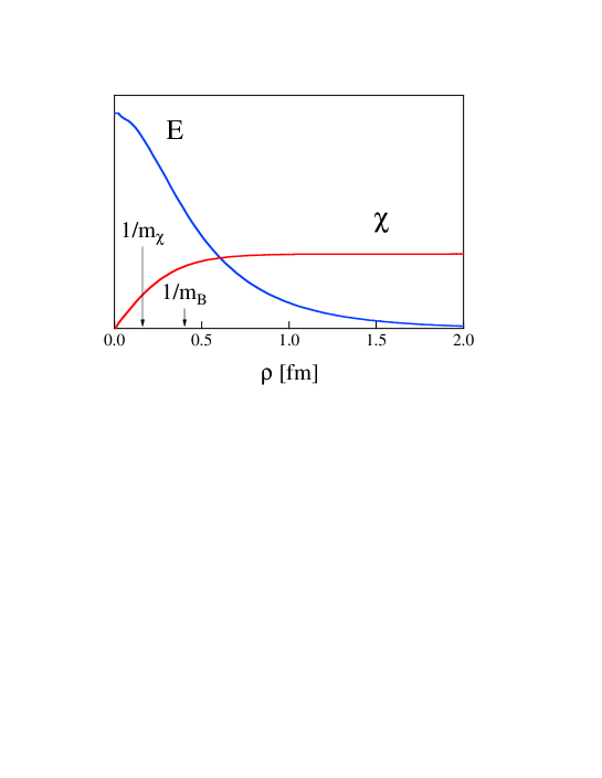
Figure 8.2: The color-electric field $E(r)$ the monopole condensate $\bar{\chi}(r)$ are plotted as the function of $r$ in the cylindrical coordinate.

We show in Fig.8.2 the profile of the color electric-field $E(r)$ and the monopole field $\chi(r)$. Apart from $r=0$, the monopole condenses, while the monopole condensate disappears near the center of flux-tube. Accordingly, the color electric-field is squeezed like a one-dimensional tube, whose radius is about $1/m_{B}$. In this way, in the QCD vacuum, there are three types of the flux-tubes according to the color of quarks, being different from the superconductivity. However, the DGL Lagrangian in the all color system becomes a simple GL type and there is a solution where the color-electric field is squeezed like a one-dimensional tube as the Abrikosov vortex. This result is consistent with the Regge trajectory of hadrons and the lattice QCD results, which indicates that the QCD vacuum can be regarded as the dual version of the superconductor.

8.5 Quark Confinement Potential

In the DGL theory, the color-electric flux between quarks is squeezed into one-dimensional tube as the result of monopole condensation. This indicates that the static potential between quark and anti-quark is linear confinement potential. Here, we investigate the interquark potential using the gluon propagator including the nonperturbative effect [33].

The static potential between heavy quarks can be obtained from the vacuum energy where the static quark and antiquark exist. Here, we take a quench approximation, i.e. we neglect the quantum effect of the light quarks. As a first step, we approximate the monopole filed $\chi_{a}$ as the mean field $|\chi_{a}|=v$ neglecting the effect of the quark sources on the condensed monopole. Later, we include the correction in order to eliminate the divergence originated from this approximation. In this scheme, information on confinement is included in the gluon propagator, which leads to the strong interaction in the infrared region.

The vacuum energy $V(j)$ in the presence of the static quark sources $j$ is obtained from

$$Z=<0|e^{i\int\vec{j}_{\mu}\vec{A}^{\mu}d{{}^{4}}x}|0>=N\int{\cal D}\vec{A}_{\mu}{\cal D}\vec{B}_{\mu}e^{i\int{({\cal L}+\vec{j}_{\mu}\vec{A}^{\mu})d^{4}x}}=e^{-iV(j)\int{dt}}.$$ (8.72)

The Lagrangian on the mean field level for the monopole field is written as

$${\cal L}_{DGL-MF} = -{1\over{2n^{2}}}[n\cdot(\partial\wedge\vec{A})]^{\nu}[n\cdot{}^{*}(\partial\wedge\vec{B})]_{\nu}+{1\over{2n^{2}}}[n\cdot(\partial\wedge\vec{B})]^{\nu}[n\cdot{}^{*}(\partial\wedge\vec{A})]_{\nu}$$ (8.73)

$$-{1\over{2n^{2}}}[n\cdot(\partial\wedge\vec{A})]^{2}-{1\over{2n^{2}}}[n\cdot(\partial\wedge\vec{B})]^{2}$$

$${+\bar{q}(i\gamma_{\mu}\partial^{\mu}-e\gamma_{\mu}\vec{A}^{\mu}\cdot\vec{H}-m)q}+{1\over 2}m_{B}^{2}\vec{B}_{\mu}^{2}.$$

Integrating out the dual gauge field $B_{\mu}$, it becomes

$${\cal L}_{DGL-MF}=-{1\over 4}\vec{f}_{\mu\nu}\vec{f}^{\mu\nu}+{1\over 2}\vec{A}^{\mu}K_{\mu\nu}\vec{A}^{\nu}{+\bar{q}(i\gamma_{\mu}\partial^{\mu}-e\gamma_{\mu}\vec{A}^{\mu}\cdot\vec{H}-m)q}$$ (8.74)

with

$$K_{\mu\nu} \equiv {{n^{2}m_{B}^{2}}\over{(n\cdot\partial)^{2}+n^{2}m_{B}^{2}}}X_{\mu\nu}$$ (8.75)

$$X^{\mu\nu} = {1\over{n^{2}}}\epsilon_{\lambda}^{\mu\alpha\beta}\epsilon^{\lambda\nu\gamma\delta}n_{\alpha}n_{\gamma}\partial_{\beta}\partial_{\delta}$$

$$= {1\over{n^{2}}}[-n^{2}\partial^{2}g^{\mu\nu}+(n\cdot\partial)^{2}g^{\mu\nu}+n^{\mu}n^{\nu}\partial^{2}-(n\cdot\partial)(n^{\mu}\partial^{\nu}+n^{\nu}\partial^{\mu})+n^{2}\partial^{\mu}\partial^{\nu}],$$

where $X_{\mu\nu}$ satisfies the relation, $X_{\mu\nu}=X_{\nu\mu}$ and $X_{\mu\nu}\partial^{\nu}=X_{\mu\nu}n^{\nu}=0$. When we introduce the external source $j$ in stead of dynamical quark part, we get

$${\cal L}_{DGL-MF} = {1\over 2}\vec{A}^{\mu}D^{-1}_{\mu\nu}\vec{A}^{\nu}+\vec{j}_{\mu}\vec{A}^{\mu}$$ (8.76)

$$= {1\over 2}(\vec{A}^{\mu}+\vec{j}_{\alpha}D^{\alpha\mu})D_{\mu\nu}^{-1}(\vec{A}^{\nu}+D^{\nu\beta}\vec{j}_{\beta})-{1\over 2}\vec{j}_{\mu}D^{\mu\nu}\vec{j}_{\nu}.$$ (8.77)

Integrating out $A_{\mu}$, we obtain the non-local current-current correlation as

$${\cal L}_{j}=-{1\over 2}\vec{j}_{\mu}D^{\mu\nu}\vec{j}_{\nu},$$ (8.78)

where the propagator of the diagonal gluons is written as

$$D_{\mu\nu}^{-1} = \left(g_{\mu\nu}\partial^{2}-(1-{1\over{\alpha_{e}}})\partial_{\mu}\partial_{\nu}\right)+{{m_{B}^{2}n^{2}}\over{(n\cdot\partial)^{2}+m_{B}^{2}n^{2}}}X_{\mu\nu}$$ (8.79)

$$D_{\mu\nu} = {1\over{\partial^{2}}}\left({g_{\mu\nu}+(\alpha_{e}-1){{\partial_{\mu}\partial_{\nu}}\over{\partial^{2}}}}\right)-{1\over{\partial^{2}}}{{m_{B}^{2}}\over{\partial^{2}+m_{B}^{2}}}{{n^{2}}\over{(n\cdot\partial)^{2}}}X_{\mu\nu}$$ (8.80)

in the Lorentz gauge $\partial_{\mu}A^{\mu}=0$. If the monopole does not condense $v=0$ or $m_{B}=0$, the second term in (8.80) disappears, and this propagator returns to familiar propagator derived in the perturbative sense. The nonperturbative effect is included in the second term. Indeed, the second term leads to the confinement potential as is shown from now on.

The generating functional is given as

$$Z=e^{i\int{{\cal L}_{j}d^{4}x}}\equiv e^{iS_{j}}=e^{-iV(j)\int{dt}}.$$ (8.81)

Now we try to estimate

$$S_{j}\equiv\int{{\cal L}_{j}d^{4}x}=-{1\over 2}\int{}\vec{j}_{\mu}D^{\mu\nu}\vec{j}_{\nu}d^{4}x.$$ (8.82)

The static source of the quark with charge $\vec{Q}_{a}$ located at $a$ and the anti-quark $\vec{Q}_{b}$ at $b$ is given by

$$\vec{j}_{\mu}(x)=-g_{\mu 0}\{{\vec{Q}_{a}\delta^{3}({\bf{x-a}})+\vec{Q}_{b}\delta^{3}({\bf{x-b}})}\}$$ (8.83)

and its Fourier transformation leads to

$$\vec{j}_{\mu}(k)=-g_{\mu 0}({\vec{Q}_{a}}e^{-i\bf k\cdot\bf a}+{\vec{Q}_{b}}e^{-i\bf k\cdot\bf b}).$$ (8.84)

Substituting the propagator (8.80) and the source (8.84) into (8.82), we get using the unit vector $n$

$$S_{j}=-{1\over 2}\int{{{d^{4}k}\over{(2\pi)^{4}}}}\vec{j}_{\mu}(-k)D^{\mu\nu}\vec{j}_{\nu}(k)$$

$$= {1\over 2}\int{{{d^{4}k}\over{(2\pi)^{4}}}}\vec{j}_{\mu}(-k)[{1\over{k^{2}-m_{B}^{2}}}g^{\mu\nu}+{{-m_{B}^{2}}\over{k^{2}-m_{B}^{2}}}{{n^{2}}\over{(n\cdot k)^{2}}}(g^{\mu\nu}-{{n^{\mu}n^{\nu}}\over{n^{2}}})]\vec{j}_{\nu}(k)$$

$$= -{1\over 2}\int{{{d^{3}k}\over{(2\pi)^{3}}}}(\vec{Q}_{a}+\vec{Q}_{b}e^{i\mbox{\boldmath k$\cdot$r}})(\vec{Q}_{a}+\vec{Q}_{b}e^{-i\mbox{\boldmath k$\cdot$r}})\times[{1\over{\mbox{\boldmath k}^{2}+m_{B}^{2}}}+{{m_{B}^{2}}\over{\mbox{\boldmath k}^{2}+m_{B}^{2}}}{1\over{(\mbox{\boldmath n$\cdot$k})^{2}}}]\int{dt},$$

where r $\equiv$b$-$a is relative vector between quark and anti-quark, and $2\pi\delta(0)=\int{dt}$ is used. Here, we take $n//{\bf r}$, because of the axial symmetry of the system and the energy minimum condition.

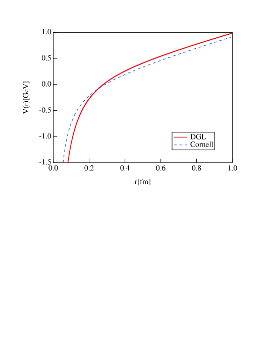
Figure 8.3: Confinement potential $V(r)$ as the function of the distance $r$ between a static quark-antiquark.

The inter-quark potential is obtained from (8.81) as

$$V(r;n)\equiv V_{\rm yukawa}(r)+V_{\rm linear}(r;n),$$ (8.86)

where the yukawa term is

$$V_{\rm yukawa}(r) = {1\over 2}\int{{{d^{3}k}\over{(2\pi)^{3}}}}(\vec{Q}_{a}+\vec{Q}_{b}e^{i{\mbox{\boldmath{k$\cdot$r}}}})(\vec{Q}_{a}+\vec{Q}_{b}e^{-i{\mbox{\boldmath k$\cdot$r}}}){1\over{\mbox{\boldmath k}^{2}+m_{B}^{2}}}$$ (8.87)

$$= \vec{Q}_{a}\cdot\vec{Q}_{b}\int{{{d^{3}k}\over{(2\pi)^{3}}}}{{e^{i{\mbox{\boldmath k$\cdot$r}}}}\over{\mbox{\boldmath k}^{2}+m_{B}^{2}}}={{\vec{Q}_{a}\cdot\vec{Q}_{b}}\over{4\pi}}{{e^{-m_{B}r}}\over r}$$

and the linear term is

$$V_{\rm linear}(r;n) = {1\over 2}\int{{{d^{3}k}\over{(2\pi)^{3}}}}(\vec{Q}_{a}+\vec{Q}_{b}e^{i\mbox{\boldmath k$\cdot$r}})(\vec{Q}_{a}+\vec{Q}_{b}e^{-i{\mbox{\boldmath k$\cdot$r}}}){{m_{B}^{2}}\over{\mbox{\boldmath k}^{2}+m_{B}^{2}}}{1\over{\mbox{\boldmath(n$\cdot$k)}}^{2}}$$ (8.88)

$$= {1\over 2}\int{{{d^{3}k}\over{(2\pi)^{3}}}}\left({\vec{Q}_{a}^{2}+\vec{Q}^{2}_{b}+2\vec{Q}_{a}\cdot\vec{Q}_{b}{\rm cos}({\mbox{\boldmath k$\cdot$r}})}\right){{m_{B}^{2}}\over{\mbox{\boldmath k}^{2}+m_{B}^{2}}}{1\over\mbox{\boldmath(n$\cdot$k)}^{2}}.$$

Introducing the ultraviolet cutoff $m_{\chi}$ corresponding to the core of the flux-tube, we get the expression,

$$V_{\rm linear}(r)={1\over{16\pi^{2}}}\int_{-\infty}^{\infty}{{{dk_{r}}\over{k_{r}^{2}}}}({\vec{Q}_{a}^{2}+\vec{Q}^{2}_{b}+2\vec{Q}_{a}\cdot\vec{Q}_{b}\cos(k_{r}r)})\ln({{m_{\chi}^{2}+k_{r}^{2}+m_{B}^{2}}\over{k_{r}^{2}+m_{B}^{2}}}),$$ (8.89)

where $k_{r}$ is parallel component of $k$ to the Dirac-string direction $n$. Since $\vec{Q}_{a}\cdot\vec{Q}_{b}$ is $-\frac{1}{3}e^{2}$ for any color system, we finally get

$$V(r)=-{e^{2}\over{12\pi}}\cdot{{e^{-m_{B}r}}\over r}+{{e^{2}m^{2}_{B}}\over{24\pi}}\ln({{m_{\chi}^{2}+m_{B}^{2}}\over{m_{B}^{2}}})r.$$ (8.90)

The string tension is given from the slope of the linear confinement potential as

$$\sigma={{e^{2}m_{B}^{2}}\over{24\pi}}\ln\left({{{m^{2}_{B}+m^{2}_{\chi}}\over{m^{2}_{B}}}}\right),$$ (8.91)

which corresponds to the vortex energy for the unit length in the typeII superconductor. Here, the gauge field mass ${m_{A}^{2}}$ is neglected in the numerator in the logarithm function, because it is much smaller than the mass of the Higgs field (Cooper-pair field), ${m_{A}^{2}}\ll{m_{\phi}^{2}}$. Thus, the confinement potential arises from the second term of the gluon propagator (8.80).

The parameters in the dual Ginzburg-Landau theory is determined so as to reproduce the interquark potential of heavy quarknium or results of the lattice QCD simulation; $e=5.5$, monopole condensate $v=0.126$GeV and interaction strength between the monopoles $\lambda=$25. These parameters lead to the unit magnetic charge $g=2.3$, the mass of the dual gauge field $m_{B}=0.5$GeV, monopole field mass $m_{\chi}=1.26$GeV and the string tension $\sigma=1.0$GeV/fm. Using these parameters, we compare in Fig.8.3 the phenomelogical potential like Cornell potential [71]

$$V_{\rm Cornell}=-{{e^{2}_{c}}\over{3\pi}}{1\over r}+\sigma_{c}r.$$ (8.92)

In the short range $r\leq 0.2$fm= (1GeV)^-1, the Coulomb term dominates, while the linear potential dominates in the longer distance.

Thus, in the DGL theory, the gluon propagator includes the long range correlation between quarks through the non-local operator $\frac{1}{(n\cdot\partial)^{2}}$. Such a long range correlation along the direction of the Dirac string leads to the linear confinement potential.

8.6 Asymptotic Behavior in DGL Theory

Finally, we discuss the gauge coupling behavior in the DGL theory in terms of the renormalization group [72]. In the abelian gauge fixing, the Dirac condition $eg=4\pi$ for the dual gauge coupling constant $g$ is derived [19, 33]. Since Dirac condition is a geometrical relation, it is renormalization group invariant. Therefore, “see-saw relation” between the gauge coupling constant $e$ and the dual gauge coupling constant $g$ is expected; a strong coupling system in one sector corresponds to a weak-coupling system in the other sector [33, 73].

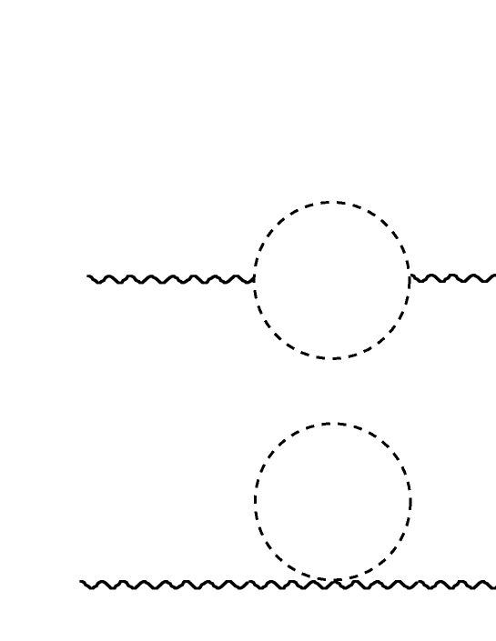
Figure 8.4: The lowest-order polarization diagrams of the dual gauge field $B_{\mu}$, which is denoted by the wavy line, in the DGL theory. The dotted line denotes the monopole field.

The DGL theory in the pure gauge is renormalizable similar to the abelian Higgs model [74], and is not asymptotically free on $g$ in view of the renormalization group: $g(p^{2})$ become large as $p^{2}$ increases. Hence, asymptotic freedom is expected for the QCD gauge coupling constant $e$ owing to the Dirac condition: $e(p^{2})$ defined by $e(p^{2})g(p^{2})=4\pi$ become small as $p^{2}$ increases. Thus, the DGL theory qualitatively shows asymptotic freedom on the QCD gauge coupling $e$ [33, 73]. This asymptotic behavior in the DGL theory is consistent with QCD qualitatively, and seems a desirable feature for an effective theory of QCD.

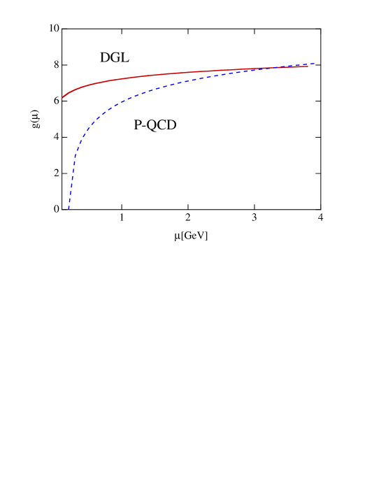
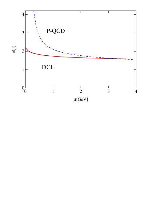
Figure 8.5: The running coupling constant $g(\mu)$ as the function of the renormalization point $\mu$. The solid curve denotes the result in the DGL theory, which is directly calculated. The dashed curve denotes the leading-order perturbative QCD result, where $g(\mu)$ is obtained using the Dirac condition $eg=4\pi$.

Figure 8.6: The running coupling constant $e(\mu)$ as the function of the renormalization point $\mu$. The solid curve denotes the result in the DGL theory, where $e(\mu)$ is obtained using the Dirac condition $eg=4\pi$. The dashed curve denotes the leading-order perturbative QCD result.

Next, we attempt to calculate the $\beta$-function and the running coupling constant from the polarization tensor $\Pi_{\mu\nu}^{ab}(p)$ of the dual gauge field $B_{\mu}$ in the DGL theory. In particular, we are interested in the infrared region ($p\leq 1{\rm GeV}$), where the perturbative QCD calculation is not reliable.

With the dimensional regularization [1, 74] by shifting the space-time dimension as $d=4-\epsilon$, we calculate the simplest nontrivial radiative correction from the monopole loop diagrams as shown in Fig.8.4,

$$\Pi_{\mu\nu}^{ab}(p)=-{1\over 32\pi^{2}}\delta^{ab}(g\mu^{-\epsilon})^{2}(p^{2}g_{\mu\nu}-p_{\mu}p_{\nu}){1\over\epsilon}+O(\epsilon^{0}),$$ (8.93)

where $g$ is the bare dual-gauge coupling and $\mu$ the renormalization point. In the minimum subtraction scheme [1], the O(1/$\epsilon$) divergence is eliminated by the counter term contribution,

$$\Pi_{\mu\nu}^{{\rm C}ab}(p)=-(Z_{3}-1)\delta^{ab}(p^{2}g_{\mu\nu}-p_{\mu}p_{\nu}),$$ (8.94)

where $Z_{3}$ is the wave-function renormalization constant [74] of the dual gauge field $B_{\mu}$,

$$Z_{3}(\mu)=1-{(g\mu^{-\epsilon})^{2}\over 32\pi^{2}}{1\over\epsilon}.$$ (8.95)

Because of the Ward identity $Z_{1}=Z_{2}$ [74], the renormalized coupling constant is simply given by $g(\mu)=Z_{3}(\mu)^{1/2}g$. The $\beta$-function [1, 74] is then expressed as

$$\beta\equiv\mu{d\over d\mu}g(\mu)=\mu{d\over d\mu}\{Z_{3}(\mu)^{1/2}g\}={1\over 32\pi^{2}}g(\mu)^{3}+O[g(\mu)^{5}],$$ (8.96)

which determines the behavior of the running coupling $g(\mu)$ as

$${1\over g^{2}(\mu)}={1\over g^{2}(\mu_{0})}-{1\over 32\pi^{2}}\ln(\mu^{2}/\mu_{0}^{2})$$ (8.97)

within the leading order.

By summation of the multi-polarization diagrams, one obtains the final formula for the running coupling $g(\mu)$ including the higher order correction,

$$g^{2}(\mu)=g^{2}(\mu_{0})-{1\over 32\pi^{2}}\ln(\mu^{2}/\mu_{0}^{2}).$$ (8.98)

In the DGL theory, the QCD gauge coupling $e(\mu)$ defined by $e(\mu)g(\mu)=4\pi$ is simply expressed as

$$e^{2}(\mu)=e^{2}(\mu_{0})\left\{1+{1\over e^{2}(\mu_{0})}\ln(\mu/\mu_{0})\right\}^{-1}.$$ (8.99)

We show in Fig.8.6 the running coupling constants, $g(\mu)$ and $e(\mu)$, in the DGL theory with the parameter set in Ref. [75]: $m_{\chi}$=1.67GeV. Similarly in QED or the abelian Higgs model, we have imposed the renormalization condition as $g(\mu=2m_{\chi})=7.9$ [ $e(\mu=2m_{\chi})=1.59$ ], which is taken to be consistent with the parameter $g=6.28$ ($e=2.0$) in Ref. [75] in the infrared region (see Fig.8.6). This result shows that the gauge coupling $e(\mu)$ behaves as “walking coupling constant”, which means the coupling varies slowly, even in the infrared region as $\mu\leq 1{\rm GeV}$.

Thus, owing to the Dirac condition $eg=4\pi$, the DGL theory has asymptotic freedom nature on the gauge coupling constant $e$, where the “walking coupling constant” is predicted for $e$ even in the infrared region.

Chapter 9 QCD Phase Transition at Finite Temperature

The QCD vacuum is non-trivial at zero temperature. In this vacuum, quarks and gluons are confined in hadrons and the chiral symmetry is spontaneously broken. As the temperature increases, however, the color degrees of freedom in hadrons are defrozen. Above the critical temperature, the QCD vacuum is in the quark-gluon plasma (QGP) phase, where quarks and gluons move almost freely.

The QCD phase transition is investigated in the various field of physics. As for the lattice QCD, the QCD phase transition is one of the most important subject in the computer science and studied using the Monte Carlo simulation. The simulation demonstrates that such a phase transition happens at about 280 MeV for the pure gauge case [76] and at about 100$\sim$200MeV for the full QCD case [77]. In the early Universe, the QCD phase transition is considered to have occurred, i.e, the system was changed from the QGP phase into the hadron phase around the 200-300 MeV as the temperature decreases. As for the actual experience, in the recent years, some experimental groups are trying to create QGP in the laboratory using high-energy heavy-ion collisions. The RHIC (Relativistic Heavy Ion Collier) project is aimed at forming QGP and at studying its properties.

In this chapter, we investigate the behavior of the color-confinement at high temperature by studying the change of the properties in the QCD vacuum with temperatures in terms of the dual Ginzburg-Landau theory [47, 78]. To this end, we concentrate on the pure-gauge QCD case, where glueballs appear as the physical excitation. Although such a pure gauge system is different from the real world, it is regarded as a proto-type of real QCD and is well studied by using the lattice QCD simulation [42]. It is worth mentioning that our framework based on the DGL theory can be extended to include the dynamical quarks straightforwardly [22, 33] keeping the chiral symmetry of the system, which is explicitly broken in the color-dielectric model [79] or in the lattice QCD with the Wilson fermion [42].

9.1 Effective Potential Formalism at Finite Temperature

In order to find the stable vacuum in the field theory, the effective potential formalism is useful [80]. The effective potential indicates the vacuum energy at zero temperature and corresponds to the thermodynamical potential at finite temperature. Here, we investigate the effective potential in the path integral formalism in the DGL theory [47]. The partition functional is written as

$$Z[J]=\int{\cal D}{\chi_{\alpha}}{\cal D}{\vec{B}_{\mu}}\exp{\left(i\int d^{4}x\{{\cal{L}}_{\rm DGL}-J\sum_{\alpha=1}^{3}|\chi_{\alpha}|^{2}\}\right)},$$ (9.1)

where we take the quadratic source term [81] instead of the standard linear source term [1, 80]. As is well-known in the $\phi^{4}$ theory [1, 80], the use of the linear source term leads to an imaginary mass of the scalar field $\chi_{\alpha}$ in the negative-curvature region of the classical potential, and therefore the effective action cannot be obtained there due to the appearance of “tachyons”. In this respect, there is an extremely advanced point in the use of the quadratic source term [81], because the mass of the scalar field $\chi_{\alpha}$ is always real even in the negative-curvature region of the classical potential owing to the contribution of the source $J$ to the scalar mass (see Eq.(9.5). Then, one obtains the effective action for the whole region of the order parameter without any difficulty of the imaginary-mass problem. Moreover, the effective action with the quadratic source can be formulated keeping the symmetry of the classical potential. Since this method with the quadratic source term is quite general, it is convenient to formulate the non-convex effective potential in the $\phi^{4}$ theory, the linear $\sigma$ model or the Higgs sector in the unified theory [1].

The vacuum expectation value of $\chi_{\alpha}$ ($\alpha$=1,2,3) is the same value $\bar{\chi}$ due to the Weyl symmetry [22], and therefore we separate the monopole field $\chi_{\alpha}$ into its mean field $\bar{\chi}$ and its fluctuation $\tilde{\chi}_{\alpha}$ as

$$\chi_{\alpha}=\left(\bar{\chi}+\tilde{\chi_{\alpha}}\right)\exp{\left(i\xi_{\alpha}\right)}.$$ (9.2)

Here, the phase variables $\xi_{\alpha}$ have a constraint, $\sum_{\alpha=1}^{3}\xi_{\alpha}=0$, where two independent degrees of freedom remain corresponding to the dual gauge symmetry $[{\rm U(1)}_{3}\times{\rm U(1)}_{8}]_{m}$ [22, 33]. When monopoles condense, the phase variables $\xi_{\alpha}$ turn into the longitudinal degrees of the dual gauge field $\vec{B}_{\mu}$, which is the dual Higgs mechanism.

Since we are interested in the translational-invariant system as the QCD vacuum, we consider the $x$-independent constant source $J$, which leads to a homogeneous monopole condensate. In the unitary gauge, the Lagrangian with the source term is rewritten as

$${\cal L}_{\rm DGL} -J\sum_{\alpha=1}^{3}|\chi_{\alpha}|^{2}={\cal L}_{\rm cl}(\bar{\chi})-3J\bar{\chi}^{2}-2\bar{\chi}[2\lambda(\bar{\chi}^{2}-v^{2})+J]\sum_{\alpha=1}^{3}\tilde{\chi}_{\alpha}$$

$$-{1\over 4}(\partial_{\mu}\vec{B}_{\nu}-\partial_{\nu}\vec{B}_{\mu})^{2}+{1\over 2}m_{B}^{2}\vec{B}_{\mu}^{2}+\sum_{\alpha=1}^{3}[(\partial_{\mu}\tilde{\chi}_{\alpha})^{2}-m_{\chi}^{2}\tilde{\chi}_{\alpha}^{2}]$$

$$+\sum_{\alpha=1}^{3}\{g^{2}(\vec{\epsilon}_{\alpha}\cdot\vec{B}_{\mu})^{2}(\tilde{\chi}_{\alpha}^{2}+2\bar{\chi}\tilde{\chi}_{\alpha})-\lambda(4\bar{\chi}\tilde{\chi}_{\alpha}^{3}+\tilde{\chi}_{\alpha}^{4})\},$$

where ${\cal L}_{\rm cl}(\bar{\chi})$ is the classical part,

$${\cal L}_{\rm cl}(\bar{\chi})=-3\lambda(\bar{\chi}^{2}-v^{2})^{2}.$$ (9.4)

Here, the masses of $\tilde{\chi}_{\alpha}$ and $\vec{B}_{\mu}$ are given by

$$m_{\chi}^{2}=2\lambda(3\bar{\chi}^{2}-v^{2})+J=4\lambda\bar{\chi}^{2},\hbox{\quad}m_{B}^{2}=3g^{2}\bar{\chi}^{2},$$ (9.5)

where we have used the relation between the mean field $\bar{\chi}$ and the source $J$,

$$J=-2\lambda(\bar{\chi}^{2}-v^{2}).$$ (9.6)

This relation is obtained by the condition that the linear term of $\tilde{\chi}_{\alpha}$ vanishes. It is remarkable that the scalar mass $m_{\chi}$ is always real owing to the source $J$ even in the negative-curvature region of the classical potential, $\bar{\chi}<v/\sqrt{3}$.

Integrating over $\vec{B}_{\mu}$ and $\tilde{\chi}_{\alpha}$ by neglecting the higher order terms of the fluctuations, we obtain the partition functional,

$$Z[J]=\exp{\left(i\int d^{4}x\{{\cal L}_{\rm cl}(\bar{\chi})-3J\bar{\chi}^{2}\}\right)}[\hbox{Det}(iD_{B}^{-1})]^{-1}[\hbox{Det}(iD_{\chi}^{-1})]^{-3/2},$$ (9.7)

where the exponents, $-1$ and $-3/2$, originate from the numbers of the internal degrees of freedom. Here, $D_{B}$ and $D_{\chi}$ are the propagators of $\vec{B}_{\mu}$ and $\tilde{\chi}_{\alpha}$ in the monopole condensed vacuum,

$$D_{B}=\left(g_{\mu\nu}-{k_{\mu}k_{\nu}\over m_{B}^{2}}\right){i\over k^{2}-m_{B}^{2}+i\epsilon},\hbox{\quad}D_{\chi}={-i\over k^{2}-m_{\chi}^{2}+i\epsilon}$$ (9.8)

in the momentum representation. Hence, the effective action is given by the Legendre transformation [1],

$$\Gamma(\bar{\chi}) = -i\ln Z[J]+\int d^{4}x3J\bar{\chi}^{2}$$ (9.9)

$$= \int d^{4}x{\cal L}_{\rm cl}(\bar{\chi})+i\ln{\rm Det}(iD_{B}^{-1})+{3\over 2}i\ln{\rm Det}(iD_{\chi}^{-1}).$$

The functional determinants are easily calculable in the momentum space, and we obtain the formal expression of the effective potential [1],

$$V_{\rm eff}(\bar{\chi})={-\Gamma(\bar{\chi})/\int d^{4}x}=3\lambda(\bar{\chi}^{2}-v^{2})^{2} +3\int{d^{4}k\over i(2\pi)^{4}}\ln(m_{B}^{2}-k^{2}-i\epsilon)$$ (9.10)

$$+{3\over 2}\int{d^{4}k\over i(2\pi)^{4}}\ln(m_{\chi}^{2}-k^{2}-i\epsilon).$$

In the finite-temperature system [80], the partition functional $Z$ is described by the Euclidean variables; $x_{0}=-i\tau$, and the upper bound of the $\tau$ integration is $\beta=1/T$ with $T$ being the temperature. Then, the $k_{0}$-integration in the functional determinant becomes the infinite sum over the Matsubara frequency [80]. The effective potential at finite temperatures physically corresponds to the thermodynamical potential, and is given by

$$V_{\rm eff}(\bar{\chi};T)=3\lambda(\bar{\chi}^{2}-v^{2})^{2} +3T\sum_{n=-\infty}^{\infty}\int{d^{3}k\over(2\pi)^{3}}\ln\{(2n\pi T)^{2}+k^{2}+m_{B}^{2}\}$$ (9.11)

$$+{3\over 2}T\sum_{n=-\infty}^{\infty}\int{d^{3}k\over(2\pi)^{3}}\ln\{(2n\pi T)^{2}+k^{2}+m_{\chi}^{2}\}$$

in the DGL theory. Performing the summation over $n$ and the angular integration, we obtain the final expression of the effective potential at finite temperatures,

$$V_{\rm eff}(\bar{\chi};T)=3\lambda(\bar{\chi}^{2}-v^{2})^{2} +3{T\over\pi^{2}}\int_{0}^{\infty}dkk^{2}\ln{\left(1-e^{-\sqrt{k^{2}+m_{B}^{2}}/T}\right)}$$ (9.12)

$$+{3\over 2}{T\over\pi^{2}}\int_{0}^{\infty}dkk^{2}\ln{\left(1-e^{-\sqrt{k^{2}+m_{\chi}^{2}}/T}\right)},$$

where $m_{B}$ and $m_{\chi}$ are functions of $\bar{\chi}$ as shown in Eq.(9.5). Here, we have dropped the $T$-independent part (quantum fluctuation), because we are interested in the thermal contribution to the QCD vacuum [82].

Before the numerical calculation, we examine the outline of the phase transition using the high-temperature (high-$T$) expansion. The effective potential is well approximated by the high-$T$ expansion, when the particle mass is much smaller than the temperature. Since the particle masses are almost zero for $|\bar{\chi}|\simeq 0$ as shown in Eq.(9.5), the high-$T$ expansion is applicable for the effective potential around $|\bar{\chi}|=0$.

The temperature-dependent part of the effective potential for bosons is expressed as

$$V_{T}(\bar{\chi};T) \equiv {T\over{\pi^{2}}}\int_{0}^{\infty}{dkk^{2}\ln(1-e^{-\sqrt{k^{2}+m^{2}}/T})}$$ (9.13)

$$= {{T^{4}}\over{\pi^{2}}}\int{dyy^{2}\ln(1-e^{-\sqrt{y^{2}+a^{2}}})},$$

with $y^{2}\equiv\frac{k^{2}}{T^{2}}$ and $a^{2}\equiv\frac{m^{2}}{T^{2}}$. In the high-$T$ expansion, $V_{T}(\bar{\chi};T)$ is expanded in powers of $a$,

$$V_{T}(\bar{\chi};T) = V(a^{2}(\bar{\chi}))\left|{{}_{a^{2}=0}+{{\partial V}\over{\partial a^{2}}}}\right.\left|{{}_{a^{2}=0}a^{2}}\right.+...$$ (9.14)

$$\approx {{T^{4}}\over{\pi^{2}}}\int_{0}^{\infty}{dyy^{2}\ln(1-e^{-y})}+{{T^{4}}\over{2\pi^{2}}}\int_{0}^{\infty}{dyy^{2}{1\over{\sqrt{y^{2}+a^{2}}}}{1\over{e^{\sqrt{y^{2}+a^{2}}}-1}}}\left|{{}_{a^{2}=0}a^{2}}\right.$$

$$= {{T^{4}}\over{\pi^{2}}}(-{{\pi^{4}}\over{45}})+{{T^{4}}\over{2\pi^{2}}}{{\pi^{2}}\over 6}({m\over T})^{2}=-{{\pi^{2}T^{4}}\over{45}}+{{T^{4}}\over{12}}({m\over T})^{2}.$$

Thus, $V_{\rm eff}$ in Eq.(9.12) is expressed as

$$V_{\rm eff}(\bar{\chi};T)\simeq 3\lambda(\bar{\chi}^{2}-v^{2})^{2}-{{\pi^{2}T^{4}}\over{10}}+{{T^{2}}\over{12}}({3\over 2}m_{\chi}^{2}+3m_{B}^{2})$$ (9.15)

in the high-$T$ expansion. As the temperature increases, the effective potential at $|\bar{\chi}|=0$ is changed from the minimum point to maximum point at the lower critical temperature

$$T_{low}=2v(\frac{6\lambda}{2\lambda+3g^{2}}),^{\frac{1}{2}}$$ (9.16)

which satisfies the flat curvature condition as

$$\frac{\partial^{2}V}{\partial\bar{\chi}^{2}}|_{\bar{\chi}=0}=0.$$ (9.17)

In fact, $V_{\rm eff}(\bar{\chi};T)$ at $\bar{\chi}=0$ is a local maximum for $T<T_{low}$, while it becomes a (local) minimum and the system is (meta-) stable for $T>T_{low}$. For the 2nd-order phase transition, $V_{\rm eff}$ has only one absolute minimum at each $T$ because of continuous variation of the order parameter, and therefore $T_{low}$ coincides the thermodynamical critical temperature $T_{c}$. On the other hand, for the 1st-order phase transition with a jump of the order parameter, there are two absolute minima at $T_{c}$, and the second minimum at $\bar{\chi}=0$ appears at the lower critical temperature $T_{low}$, so that $T_{low}$ is lower than $T_{c}$. In any case, using the high-$T$ expansion, we derive the analytical expression for $T_{low}$, which provides a lower bound for the critical temperature.

9.2 Numerical Results on QCD Phase Transition

Here, we show the results on the QCD phase transition which obtained from the numerical calculation [47].

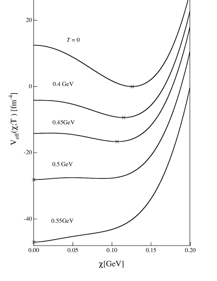
Figure 9.1: The effective potentials at various temperatures as functions of the monopole condensate $\bar{\chi}$. The numbers beside each curve are the temperatures. The absolute minimum points of the effective potentials are shown by crosses.

We first show in Fig.9.1 the effective potential at various temperatures (thermodynamical potential), $V_{\rm eff}(\bar{\chi};T)$, as a function of the monopole condensate $\bar{\chi}$, an order parameter for the color confinement. The parameters, $\lambda$ = 25, $v$ = 0.126GeV and $g$ = 2.3, are extracted by fitting the static potential in the DGL theory to the Cornell potential . These values provide $m_{B}$ = 0.5GeV and $m_{\chi}$ = 1.26GeV at $T$ = 0. The (local-)minimum point of $V_{\rm eff}(\bar{\chi};T)$ corresponds to the physical (meta-)stable vacuum state. As the temperature increases, the broken dual gauge symmetry tends to be restored, and the monopole condensate in the physical vacuum, $\bar{\chi}_{\rm phys}(T)$, is decreased. A first order phase transition is found at the thermodynamical critical temperature, $T_{C}\simeq 0.49$ GeV, and the QCD vacuum becomes trivial, $\bar{\chi}_{\rm phys}(T)=0$, for $T\geq T_{C}$. This phase transition is regarded as the deconfinement phase transition, because there is no confining force among colored particles in the QCD vacuum with $\bar{\chi}_{\rm phys}(T)=0$.

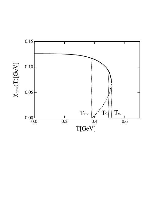
Figure 9.2: The monopole condensate $\bar{\chi}_{\rm phys}(T)$ at minima of the effective potential as a function of the temperature $T$. The solid curve denotes $\bar{\chi}_{\rm phys}(T)$ corresponding to the confinement phase, which is the absolute minimum up to $T_{C}=$0.49 GeV and becomes a local minimum up to $T_{\rm up}=$0.51 GeV. A minimum appears at $\bar{\chi}=0$ above $T_{\rm low}=$0.38 GeV and becomes the absolute minimum above $T_{C}=$0.49 GeV. The dot-dashed curve denotes the value of $\bar{\chi}$ at the local maximum.

We show the behavior of the monopole condensate in the physical vacuum, $\bar{\chi}_{\rm phys}(T)$, as a function of the temperature $T$ in Fig.9.2. One finds $\bar{\chi}_{\rm phys}$= 0.126 GeV at $T=0$, and the monopole condensate decreases monotonously up to $\bar{\chi}_{\rm phys}$ = 0.07 GeV at the upper critical temperature $T_{\rm up}=$ 0.51 GeV, where the minimum at finite $\bar{\chi}$ disappears in $V_{\rm eff}(\bar{\chi};T)$. On the other hand, the local minimum is developed at $\bar{\chi}$ = 0 in $V_{\rm eff}(\bar{\chi};T)$ above the lower critical temperature $T_{\rm low}=$ 0.38 GeV, which is analytically obtained by using the high-temperature expansion in previous section [80, 82]. The minimum value of $V_{\rm eff}(\bar{\chi};T)$ at $\bar{\chi}=0$ becomes deeper than that at finite $\bar{\chi}$ above the thermodynamical critical temperature $T_{C}$ = 0.49 GeV. Here, we get the first-order phase transition because we have considered full orders in $\bar{\chi}^{2}$ as shown in Eq.(9.12). On the other hand, Monden et al [82] did not get the first-order phase transition due to the use of only the lowest order in $\bar{\chi}^{2}$ in the high-temperature expansion [80], and therefore they had to introduce the cubic term in $\chi_{\alpha}$ in the Lagrangian.

Figure 9.3: The monopole condensate $\bar{\chi}_{\rm phys}(T)$ at minima of the effective potential as a function of the temperature in the case of variable $\lambda(T)$ so as to reproduce $T_{C}=$0.28GeV. The meanings of the curves are the same as in Fig.9.2.

Here, we consider the possibility of the temperature dependence on the parameters ($\lambda$,$v$) in the DGL theory. The critical temperature, $T_{C}$ = 0.49 GeV, seems much larger than one of the recent lattice QCD prediction, $T_{C}=0.26\sim 0.28$GeV, which is, for instance, estimated from the relation, $T_{C}/\sqrt{\sigma}\simeq 0.62$ [83] and the string tension $\sigma=0.89\sim 1.0$GeV/fm. However, we should remember that the self-interaction term of $\chi_{\alpha}$ has been introduced phenomenologically in the DGL Lagrangian. In particular, the asymptotic freedom behavior of QCD leads to a possible reduction of the self-interaction among monopoles at high temperatures. Hence, we use a simple ansatz for the temperature dependence on $\lambda$,

$$\lambda(T)=\lambda\left({T_{C}-aT\over T_{C}}\right),$$ (9.18)

keeping the other parameter $v$ constant. Here, the constant $a$ is determined as $a=0.89$ so as to reproduce $T_{C}=0.28$GeV. (We take $\lambda(T)=0$ for $T>T_{C}/a$.) The results for the monopole condensate $\bar{\chi}_{\rm phys}(T)$ are shown in Fig.9.3. The qualitative behavior is the same as in the above argument with a constant $\lambda$. We find a weak first-order phase transition in this case also. Here, we find a large reduction of the self-interaction of the monopoles near the critical temperature $T_{C}$: $\lambda(T\simeq T_{C})\simeq 2.7$ is considerably smaller than $\lambda(T=0)=25$.

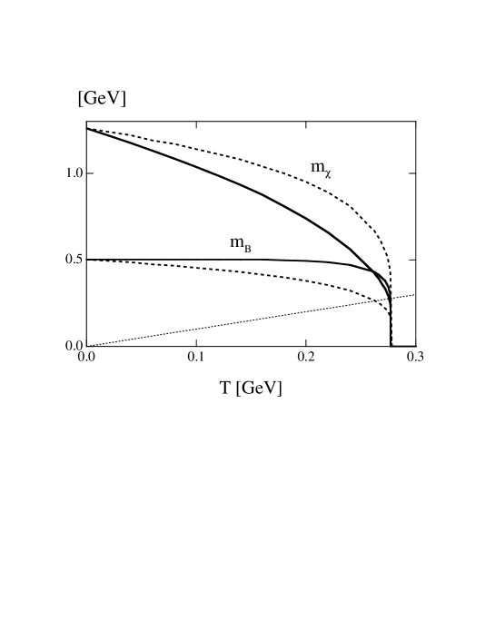
Figure 9.4: The dual gauge field mass $m_{B}(T)$ and the monopole field mass $m_{\chi}(T)$. The solid lines denote the case of variable $\lambda(T)$ with a constant $v$. The dashed lines denote the case of variable $v(T)$ with a constant $\lambda$. A large reduction of these masses is found near the critical temperature. The dotted line denotes $m=T$. The phase transition occurs at the temperature satisfying $m_{B},m_{\chi}\simeq T$.

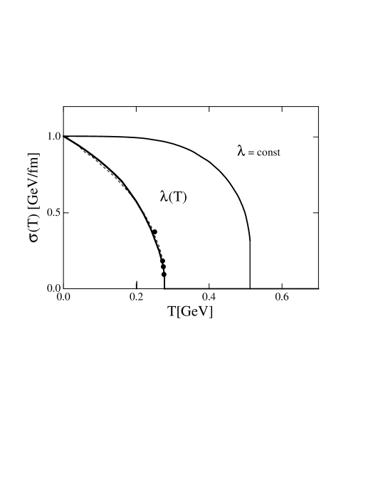
Figure 9.5: The string tension $\sigma(T)$ as a function of the temperature $T$. The solid and dashed lines correspond to the variable $\lambda(T)$ case with a constant $v$ and the variable $v(T)$ case with a constant $\lambda$, respectively. The constant ($\lambda$, $v$) case is also shown by the thin line. The lattice QCD results in the pure gauge are shown by black dots near the critical temperature.

Next, we investigate the variation of the masses of the dual gauge field $\vec{B}_{\mu}$ and the monopole field $\tilde{\chi}_{\alpha}$ at finite temperatures. Here, $\tilde{\chi}_{\alpha}$ would appear as the color-singlet glueball field with $0^{+}$ [22, 73]. These masses $m_{B}$ and $m_{\chi}$, at the finite temperature $T$ are given by

$$m_{B}(T)=\sqrt{3}g\bar{\chi}_{\rm phys}(T),\hbox{\quad}m_{\chi}(T)=2\sqrt{\lambda(T)}\bar{\chi}_{\rm phys}(T)$$ (9.19)

as shown in Eq.(9.5). In Fig.9.4, we show $m_{B}(T)$ and $m_{\chi}(T)$ as functions of the temperature $T$ using variable $\lambda(T)$ in Eq.(9.18). (Their behaviors are almost the same as the case of a constant $\lambda$ except for the difference of the value of $T_{C}$.) It is worth mentioning that $m_{B}(T)$ and $m_{\chi}(T)$ drop down to $m_{B},m_{\chi}\sim T_{C}$(=0.28GeV) from $m_{B},m_{\chi}\sim$ 1 GeV near the critical temperature $T_{C}$. In other words, the QCD phase transition occurs at the temperature satisfying $m_{B},m_{\chi}\simeq T$, which seems quite natural because the thermodynamical factor $1/\{\exp(\sqrt{k^{2}+m^{2}}/T)\pm 1\}$ becomes relevant only for $m\stackrel{{\scriptstyle<}}{{\sim}}T$. Thus, our result predicts a large reduction of the dual gauge field mass $m_{B}$ and the monopole field mass $m_{\chi}$ near the critical temperature $T_{C}$. It is desirable to study the change of the scalar glueball mass at finite temperatures, especially near $T_{C}$, in the lattice QCD simulation with the larger lattice size and the higher accuracy.

We investigate the string tension $\sigma$ at finite temperatures, since $\sigma$ is one of the most important variables for the color confinement, and controls the hadron properties through the inter-quark potential. We use the expression of the string tension $\sigma(T)$ provided by SST [33],

$$\sigma(T)={e^{2}m_{B}^{2}(T)\over 24\pi}\ln\left({m_{B}^{2}(T)+m_{\chi}^{2}(T)\over m_{B}^{2}(T)}\right),$$ (9.20)

where the masses $m_{B}(T)$ and $m_{\chi}(T)$ are given by Eq.(9.19). The results are shown in Fig.9.5 as a function of the temperature $T$. In the case of constant $\lambda$, the string tension $\sigma(T)$ decreases very gradually up to the temperature, $T_{\rm up}$= 0.51 GeV. On the other hand, in the case of variable $\lambda(T)$, the string tension $\sigma(T)$ decreases rapidly with temperature, and $\sigma(T)$ drops down to zero around $T_{C}=$ 0.28 GeV. Hence, one expects a rapid change of the masses and the sizes of the quarkonia according to the large reduction of $\sigma(T)$ at high temperatures. We plot also the pure-gauge lattice QCD results for the temperature dependence of the string tension by black dots [84], with $T_{C}=0.28$GeV [83]. We find our results with variable $\lambda(T)$ agree with the lattice QCD data.

We discuss further the temperature dependence of the parameters ($\lambda$,$v$) in the DGL theory. Definitely, we should follow the lattice QCD data for this determination as the case of the Ginzburg-Landau theory of superconductors extracting the temperature dependence from experiments. Since there exists the lattice QCD data on the string tension $\sigma$ [84], we try to reproduce $\sigma$ by taking a simple ansatz on $\lambda$ and $v$. We try the following ansatz,

$$B(T)\equiv 3\lambda(T)v^{4}(T)=3\lambda v^{4}\left({T_{C}-aT\over T_{C}}\right),$$ (9.21)

where the constant $a$ is determined so as to reproduce $T_{C}=0.28$GeV. (We take $B(T)=0$ for $T>T_{C}/a$.) The variable $B(T)$ corresponds to the bag constant, the energy-density difference between the nonperturbative vacuum ($|\chi_{\alpha}|\neq 0$) and the perturbative vacuum ($|\chi_{\alpha}|=0$) in the DGL theory; see Eq.(9.12). The ansatz (9.21) suggests the reduction of the bag constant at high temperatures, which provides the swelling of hot hadrons by way of the bag-model picture. Since we have already examined a typical case for variable $\lambda(T)$ keeping $v$ constant, we show here another typical case for variable $v(T)$ keeping $\lambda$ constant. The string tension $\sigma(T)$ in the variable $v(T)$ case with $a=0.91$ is shown by the dashed line in Fig.9.5. We find almost an identical result and find again a good agreement with the lattice QCD data. Other combinations on $\lambda(T)$ and $v(T)$ under the relation (9.21) also provide equally good results on $\sigma(T)$.

Finally, we investigate the relation between the scalar glueball mass $m_{\chi}(T)$ and the string tension $\sigma(T)$. For variable $\lambda(T)$ keeping $v$ constant, one finds from Eq.(9.20) an approximate relation,

$${m_{\chi}(T)\over\sqrt{\sigma(T)}}\simeq{(24\pi)^{1/2}\over e}\simeq 1.6,$$ (9.22)

near the critical temperature $T_{C}$. On the other hand, for variable $v(T)$ keeping $\lambda$ constant, the scalar glueball mass at finite temperatures, $m_{\chi}(T)$, is shown by the dashed line in Fig.9.4, and Eq.(9.20) leads to a simple relation,

$${m_{\chi}(T)\over\sqrt{\sigma(T)}}=\left({2\lambda\over\pi\ln\{(3g^{2}+4\lambda)/3g^{2}\}}\right)^{1/2}\simeq 3.0,$$ (9.23)

for the whole region of $T$. Thus, the DGL theory suggests a proportional relation between the scalar glueball mass and the square root of the string tension at least near $T_{C}$. It is worth mentioning that Engels et al. [83] obtained a similar relation, $m_{\rm GB}(T)=(1.7\pm 0.5)\sqrt{\sigma(T)}$, for the lowest scalar glueball at finite temperatures from the thermodynamical study on the SU(2) lattice gauge theory. Eqs.(9.22) and (9.23) can be examined from the thermodynamical study on the glueball mass in the lattice QCD, which may also reveal $T$-dependence on the parameters in the DGL theory.

9.3 Hadron Bubble Formation in Early Universe

The remaining part of this section, we consider the application of the DGL theory to big bang [78]. As Witten proposed [85], if the QCD phase transition is of first order, the hadron and the QGP phase should coexist in early Universe. Such a mixed phase may cause the inhomogeneity of the Universe in the baryon number distribution. This inhomogeneity affects the primordial nucleo-synthesis [86].

As a result of the 1st order phase transition, hadron bubbles appear in the QGP phase near the critical temperature. We now consider how hadron bubbles are formed in the DGL theory. In the supercooling system, the free energy of the hadron bubble with radius $R$ profile $\bar{\chi}(r;R)$ is written using the effective potential at finite temperature,

$$E[\bar{\chi}(r;R)]=4\pi\int_{0}^{\infty}drr^{2}\{3(\frac{d\bar{\chi}(r;R)}{dr})^{2}+V_{\rm eff}(\bar{\chi};T)\}.$$ (9.24)

We use the sine-Gordon kink ansatz for the profile of the monopole condensate,

$$\bar{\chi}(r;R)=\bar{\chi}_{H}\tan^{-1}e^{(R-r)/\delta}/\tan^{-1}e^{R/\delta},$$ (9.25)

where the thickness of the surface $\delta$ is determined by the free energy minimum conditions. The result is shown in Fig.9.7. The monopole condensate $\bar{\chi}(r;R)$ is connected smoothly between inside and outside the bubble. The energy density of the hadron bubble is shown in Fig.9.7. It is negative inside and positive near the boundary surface. The total energy is roughly estimated as the sum of the surface term (corresponding to the positive region near the surface) and the volume term (corresponding to the negative region inside the bubble).

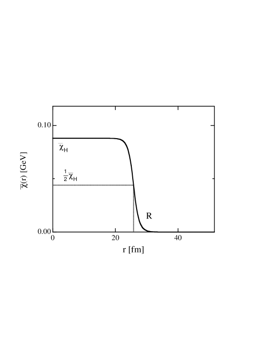
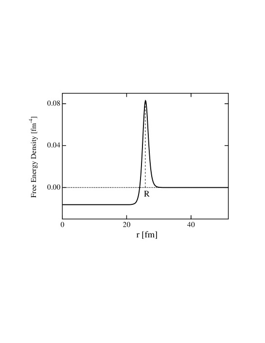
Figure 9.6: The profile of the monopole condensate in the hadron bubble. There is the QGP phase without monopole condensation outside the bubble, while hadron phase with monopole condensation remains inside the bubble.

Figure 9.7: The energy density of the hadron bubble. It is negative inside and positive near the boundary surface.

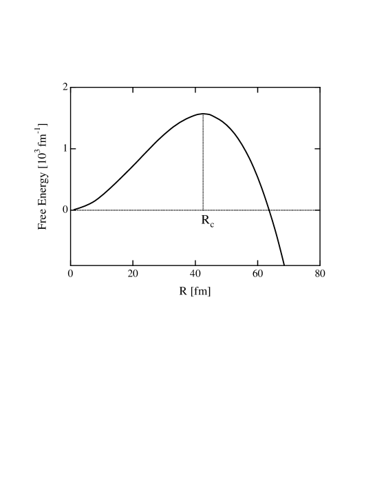
Figure 9.8: The total energy of the bubble is plotted as a function of the hadron bubble radius$R$. The total energy is roughly estimated as the sum of the volume term and the surface term.

Figure 9.9: The critical radius $R_{c}$, corresponding to maximum of the energy in Fig.9.9, is plotted as a function of temperature.

The energy of the hadron bubble with radius $R$ is shown in Fig.9.9. The bubble whose radius is smaller than critical radius $R_{c}$ collapses. Only larger bubbles ( $R>R_{c}$) are found to grow up from the energetical argument. However, the creation of large bubbles is suppressed because of formation probability. In the bubble formation process, there exists a large barrier height $h$ of the effective potential and therefore the creation of large bubbles needs the large energy fluctuation above the barrier height. Such a process is suppressed because of the thermal dynamical factor (proportional to bubble formation rate), ${\rm exp}(-\frac{4}{3}\pi R_{\rm c}^{3}h/T)$. Thus, the only small bubbles are created practically, although its radius should be larger than $R_{\rm c}$ energitically. The temperature dependence of the critical radius is shown in Fig.9.9. In the temperature region of the supercooling state, i.e, $T_{\rm low}<T<T_{\rm c}$, the hadron bubbles are created. As the temperature decreases, the size of hadron bubble becomes smaller, however the bubble formation rate becomes larger.

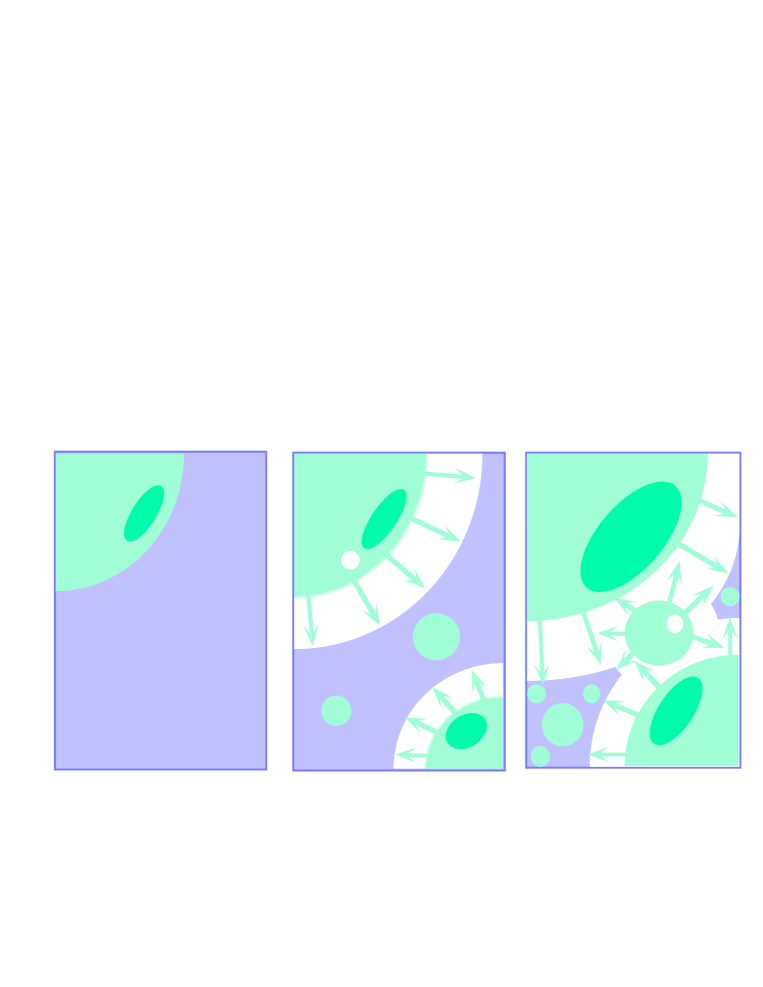
Figure 9.10: The scenario of the QCD phase transition in the early universe. The shaded and white regions denote the hadron and QGP phases, respectively. (a) Slightly below $T_{c}$, only large hadron bubbles appear with very small creation rate. (b) Hadron bubbles expand with radiating shock wave. (c) Near $T_{\rm low}$, many small hadron bubbles are created. (d) The QGP phase pressured by the hadron phase is isolated.

From these results, we can imagine how the QCD phase transition happens in the big bang scenario [87], as shown in Fig.9.10. At the first stage slightly below $T_{\rm c}$, only large bubbles are created but its rate is quite small. As temperature is lowered, smaller bubbles are created with much formation rate. During this process, the created hadron bubbles expand with radiating shock wave which reheats QGP phase [87]. Near $T_{\rm low}$ many small bubbles are violently created. Finally QGP phase is isolated like the bubble [87]. Such an evolution of the hadron bubble can be obtained from the numerical simulation using the DGL theory.

Thus, using the quadratic source term instead of the linear source term, we have obtained the effective potential in the DGL theory in the all $|\chi|$ region. Thermal effects reduce the monopole condensate and lead to deconfinement phase transition. Since the critical temperature is found very large, $T_{c}\sim 0.5$GeV, with the parameters unchanged at finite temperature, we introduce a large reduction of the self-interaction between monopoles so as to make the phase transition temperature about 0.28GeV, which is suggested in the lattice QCD. We find large reduction of string tension with the temperature in accordance with the lattice QCD results. We predict that the glueball mass decreases considerably near the critical temperature, which is to be checked by lattice QCD simulation and experiment. Based on this effective potential at finite temperature, we further investigated properties of hadron bubbles created in the early Universe and discussed the hadron bubble formation process from estimation of the size of hadron bubble at various temperatures.

Chapter 10 Application to Quark Gluon Plasma

In the recent years, some experimental groups are trying to create quark gluon plasma (QGP) as the new form of matter in the laboratory by high-energy heavy-ion collisions. The RHIC (Relativistic Heavy Ion Collier) project will start in the next year. The scenario of producing QGP is based on Bjorken’s picture [88]. Just after heavy ions pass through each other, many color-flux-tubes are produced between the projectile and the target, and pulled by them as shown in Fig.10.1(a). Usually, it is guessed that these flux-tubes are cut into several pieces through quark-antiquark pair creations, and these short flux-tubes, which behave as excited ’mesons’, are thermalized by stochastic collisions among themselves. If the energy deposition is larger than a critical value, the thermalized system becomes the QGP phase, whereas if it is lower, the system remains to be the hadron phase.

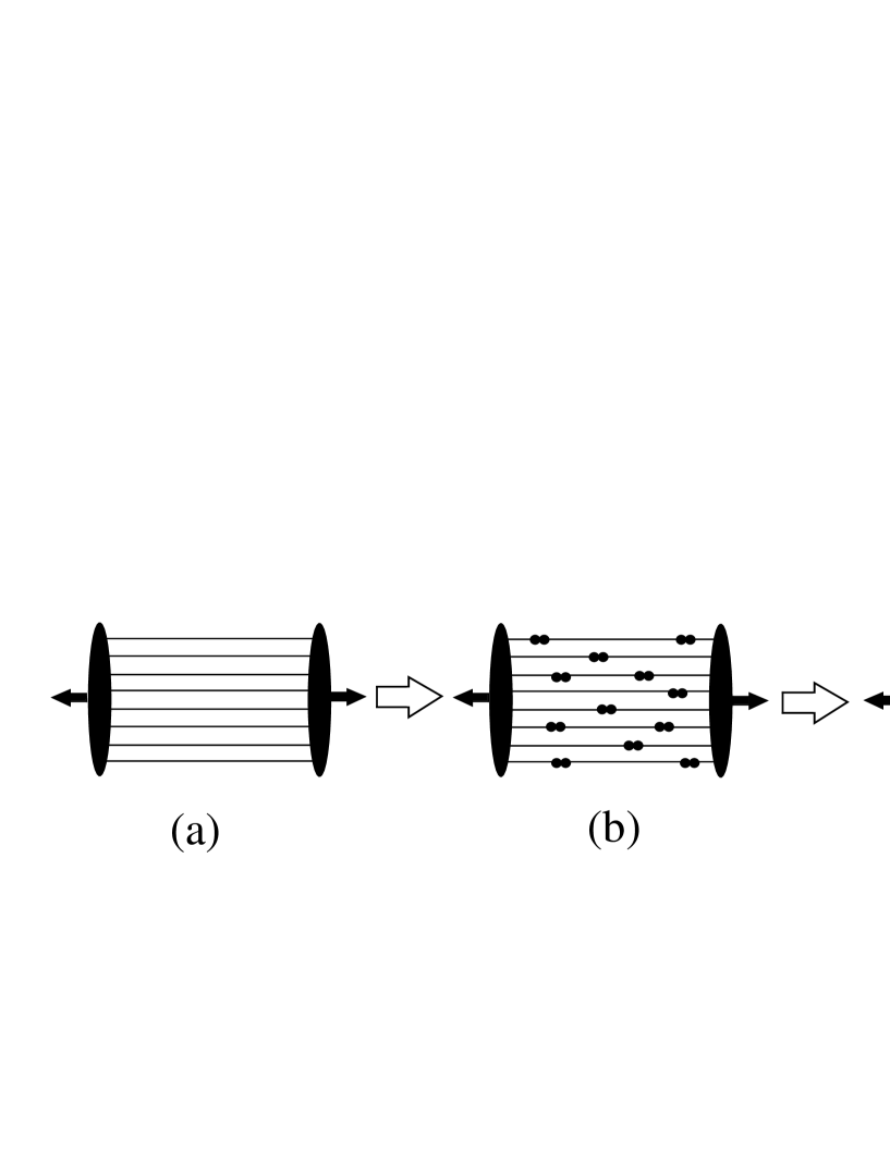
Figure 10.1: The scenario of the QGP formation in high-energy heavy-ion collisions. (a) There appear many color-flux-tubes between the projectile nucleus and the target nucleus just after the collision. (b) When the distance between the two nuclei becomes large, There appears the pair creation of quark and anti-quark. (c) Many created quarks and anti-quarks make frequent collisions to form a thermal equilibrium and form QGP, when the energy density is larger than a critical value.

The features of the multi color–flux-tube system strongly depend on their density of the flux-tubes created by hard process in early stage. When the flux-tube number density is low enough, the system is approximated as the incoherent sum of the individual flux-tube. Its evolution is expected to be superposition of random multiple hadron creations of many color-flux-tubes produced between many nucleon-nucleon pairs. On the other hand, when the flux-tube number density is sufficiently high, many flux-tubes overlap each other and would be melted into a big flux-tube. During this process, each flux-tube loses its individuality and the whole system can be regarded as a huge flux-tube between heavy-ions like a condenser [89].

In this chapter, we would like to study the properties of the multi-flux-tube system [90]. QCD is very hard to deal with in the infrared region analytically due to the breakdown of the perturbation technique. Moreover, for such a large scale system there is a severe limit on the computational power even in the lattice QCD simulation. For the study of the QGP formation, the DGL theory would provide a useful method, because it describes the properties of the color-electric flux tube, which are important in the pre-equillibrium system just after the ultrarelativistic heavy-ion collisions.

10.1 Formalism on Multi-flux-tube System

In this section, we formulate the multi-flux-tube system in the DGL theory. In this theory, the color-flux-tube is described as the dual version of the Abrikosov vortex [70]. Different from the multi-vortex system in the superconductor, however, there are some kinds of the color-flux-tubes corresponding to the kinds of color. Furthermore, in the superconductor, the direction of the flux-tube is all same and the system can be described only by the ground state such as triangle lattice system, while in the QCD vacuum many color flux-tubes distribute randomly and the system includes the highly excited states. Here, we simplify such a complex system and discuss qualitatively. For simplicity, we consider a single color charge system using the dual Ginzburg-Landau Lagrangian Eq.(8.67).

We consider two ideal cases of multi-flux-tube penetrating on a two dimensional plane. The directions of all the color-flux-tubes are the same [Fig.10.2(a)] in one case or alternative[Fig.10.2(b)] in the other case. When the flux-tubes are long enough, the effect of the flux edges is negligible. Hence, taking the direction of the flux-tubes as the $z$-axis, the system is translationally invariant in the $z$-direction and is essentially described only with two spatial coordinates $(x,y)$. For the periodic case in the $(x,y)$ coordinate, we can regard the system as two flux-tubes going through two poles (north and south poles) of the $S^{2}$ sphere. For the system of flux-tubes with all the directions being the same, we take two flux-tubes passing through the two poles on $S^{2}$ sphere as shown in Fig.10.2(a) (which we call the two flux-tubes system). For the alternative case, on the other hand, we take a flux-tube coming in from the south pole and the other leaving out through the north pole (which we call flux-tube and anti-flux-tube system). Such a prescription leads the exact solution for the periodic crystal of the sine-Gordon kinks, and also provides a simple but good description for the finite density Skyrmion system studied by Manton [92].

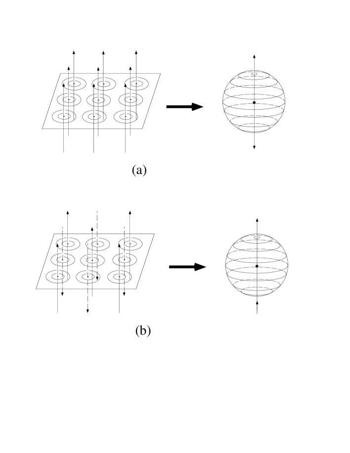
Figure 10.2: (a) A multi-flux-tube system with the same direction of the flux-tubes is approximated by the two color-flux-tubes going out from the north and the south poles on a sphere $S^{2}$. (b) A multi-flux-tube system, where flux-tube direction is alternative, is approximated by the flux-tube and ’anti-flux-tube’ system penetrating on $S^{2}$ with the color-flux going in from the south pole and leaving out from the north pole.

The two color-flux-tube system on the sphere $S^{2}$ with radius $R$ corresponds to the multi-flux-tube system with the density $\rho=1/(2\pi R^{2})$. Introducing the polar coordinates $(R,\theta,\varphi)$ on $S^{2}$, we consider the static solution satisfying

$$B_{0}=0,\hskip 56.9055pt{\bf B}=B(\theta){\bf e}_{\varphi}\equiv\frac{\tilde{B}(\theta)}{R\sin\theta}{\bf e}_{\varphi},\hskip 56.9055pt\chi=\bar{\chi}(\theta)e^{in\varphi},$$ (10.1)

where we have used the axial symmetry of the system. Here the electric field penetrates vertically on the sphere surface, ${\bf E}//{\bf e}_{r}$;

$${\bf E}={\bf\nabla}\times{\bf B}=E{\bf e}_{r},$$ (10.2)

which corresponds to the electric field penetrating vertically on the plane, ${\bf E}//{\bf e}_{z}$. The field equations are given by

$${1\over{R^{2}\sin\theta}}{d\over{d\theta}}(\sin\theta{{d\bar{\chi}}\over{d\theta}})-[{1\over{R^{2}\sin^{2}\theta}}(n-g\tilde{B}(\theta))^{2}+2\lambda(\bar{\chi}^{2}-v^{2})]\bar{\chi}=0,$$ (10.3)

$${d\over{R^{2}d\theta}}({1\over{\sin\theta}}{d\over{d\theta}}\tilde{B}(\theta))+\frac{2g}{\sin\theta}(n-g\tilde{B}(\theta))\bar{\chi}^{2}=0.$$ (10.4)

Consider the closed loop $C$ on $S^{2}$ with a constant polar angle $\theta=\alpha$ and $\phi\in[0,2\pi)$, the electric flux penetrating the area surrounded by the loop $C$ is given by

$$\Phi(\alpha)=\int_{S}{\bf E}\cdot d{\bf S}=\int{\bf\nabla}\times{\bf B}\cdot d{\bf S}=\oint_{c}{\bf B}\cdot d{\bf l}=2\pi\tilde{B}(\alpha).$$ (10.5)

The boundary conditions for the two flux-tubes system as shown in Fig.10.2(a) are given as

$$\Phi(\alpha)=2\pi\tilde{B}(\alpha)=0,\hskip 56.9055pt\bar{\chi}(\alpha)=0\hskip 56.9055pt{\rm as}\hskip 14.22636pt\alpha\rightarrow 0,$$ (10.6)

$$\Phi(\alpha)=2\pi\tilde{B}(\alpha)=\frac{1}{2}\int_{S}ER^{2}d\Omega=\pm\frac{2\pi n}{g}\hskip 56.9055pt{\rm as}\hskip 14.22636pt\alpha\rightarrow\frac{\pi}{2}\pm\epsilon,$$ (10.7)

Here, $n$ corresponds to the topological number of the flux-tube, which appears also in the vortex solution in the superconductivity. This boundary condition at $\alpha\rightarrow\frac{\pi}{2}\pm\epsilon$ has a discontinuity for the dual gauge field $\tilde{B}$. Because the electric flux leaves out from the two poles, there should be some sources to provide the electric flux. In this case, the Dirac-string like singularity appears on the $\theta=\pi/2$ line, through which the electric flux comes into the sphere from long distance. For the flux-tube and anti-flux-tube system as shown in Fig.10.2(b), the boundary condition around $\theta=0,\pi$ is given as

$$\Phi(\alpha)=2\pi\tilde{B}(\alpha)=0,\hskip 56.9055pt\bar{\chi}(\alpha)=0\hskip 56.9055pt{\rm as}\hskip 14.22636pt\alpha\rightarrow 0,\pi.$$ (10.8)

In this case, there does not appear the Dirac-string like singularity, since the electric flux is conserved. The free energy for the unit length of the color-flux-tube is written as

$$F = \int{R^{2}d\Omega}\left[{{1\over 2}\left({{1\over{R^{2}\sin\theta}}{d\over{d\theta}}\tilde{B}(\theta)}\right)^{2}+\left({{1\over R}{{d\bar{\chi}}\over{d\theta}}}\right)^{2}}\right]$$ (10.9)

$$+ \int{R^{2}d\Omega}\left[{{1\over{R^{2}\sin^{2}\theta}}(n-g\tilde{B}(\theta))^{2}\bar{\chi}^{2}+\lambda\left({\bar{\chi}^{2}-v^{2}}\right)^{2}}\right]$$

$$= \int_{0}^{\theta=\pi}{2\pi\sin}\theta d\theta\left[{\left({{{d\bar{\chi}}\over{d\theta}}}\right)^{2}+{1\over{\sin^{2}\theta}}(n-g\tilde{B}(\theta))\bar{\chi}^{2}}\right]$$

$$+ \int_{0}^{\theta=\pi}{2\pi\sin}\theta d\theta\left[{{1\over 2}\left({{1\over{\sin\theta}}{d\over{d\theta}}\tilde{B}(\theta)}\right)^{2}}\right]\cdot{1\over{R^{2}}}$$

$$+ \int_{0}^{\theta=\pi}{2\pi\sin}\theta d\theta\left[{\lambda\left({\bar{\chi}^{2}-v^{2}}\right)^{2}}\right]\cdot R^{2}.$$

First, we consider a limit of $R\rightarrow\infty$, which corresponds to the ordinary single vortex solution. Introducing a new variable $\rho\equiv R\sin\theta$, the free energy in the limit $R\gg\rho$$(\theta\sim 0)$ is written as

$$F = \int{2\pi\rho d\rho}\left[{{1\over 2}\left({{1\over\rho}{d\over{d\rho}}\rho B(\rho)}\right)^{2}+\left({{{d\bar{\chi}}\over{d\rho}}}\right)^{2}}\right]$$ (10.10)

$$+ \int{2\pi\rho d\rho}\left[{{1\over{\rho^{2}}}(n-g\rho B(\rho))\bar{\chi}^{2}+\lambda\left({\bar{\chi}^{2}-v^{2}}\right)^{2}}\right],$$

and the field equations are

$${1\over\rho}{d\over{d\rho}}\rho\left({{d\over{d\rho}}\bar{\chi}}\right)-{1\over{\rho^{2}}}(n-g\rho B(\rho))^{2}-2\lambda\left({\bar{\chi}^{2}-v^{2}}\right)\bar{\chi}=0,$$ (10.11)

$${d\over{d\rho}}{1\over\rho}{d\over{d\rho}}\left({\rho B(\rho)}\right)+{{2g}\over{\rho}}(n-g\rho B(\rho))\bar{\chi}^{2}=0,$$ (10.12)

with the boundary condition,

$$\Phi=2\pi\rho B(\rho)|^{\infty}_{0}=\frac{2\pi n}{g}\hskip 14.22636pt\mbox{as}\hskip 14.22636pt\rho\rightarrow\infty.$$ (10.13)

Above equations, (10.10-10.12), coincide exactly with those of ordinary single vortex solution in the cylindrical coordinate. Thus, we get the desired results.

One can analytically investigate the dependence of the profile functions$(\tilde{B}(\theta),\chi(\theta))$ on the flux-tube number density. For this purpose, we express the free energy as

$$F\equiv f_{0}+f_{E}\cdot{1\over{R^{2}}}+f_{\chi}\cdot R^{2},$$ (10.14)

where $f_{0},f_{E},$ and$f_{\chi}$ are $R$ independent functions and written as

$$f_{0} \equiv \int_{0}^{\theta=\pi}{2\pi\sin}\theta d\theta\left[{\left({{{d\bar{\chi}}\over{d\theta}}}\right)^{2}+{1\over{\sin^{2}\theta}}(n-g\tilde{B}(\theta))^{2}\bar{\chi}^{2}}\right],$$ (10.15)

$$f_{E} \equiv \int_{0}^{\theta=\pi}{2\pi\sin}\theta d\theta{{1\over 2}\left({{1\over{\sin\theta}}{d\over{d\theta}}\tilde{B}(\theta)}\right)^{2}},$$ (10.16)

$$f_{\chi} \equiv \int_{0}^{\theta=\pi}{2\pi\sin}\theta d\theta{\lambda\left({\bar{\chi}^{2}-v^{2}}\right)^{2}}.$$ (10.17)

In the large $R$ case, which corresponds to the small color-flux-tube number density in the original multi-flux-tube system, the third term $f_{\chi}R^{2}$ is dominant. Hence, the free energy $F$ is minimized as $\bar{\chi}\sim v$, that is, the monopole tends to condense, and then the color electric field is localized only around $\theta=0$ (north pole) and $\theta=\pi$ (south pole) as shown in Fig.10.3. On the other hand, in the small $R$ case, the second term ${f_{E}}/{R^{2}}$ is dominant. There is a constraint on the total flux penetrating on the upper sphere,

$$\Phi\equiv\int^{\frac{\pi}{2}}_{0}E(\theta)2\pi R^{2}{\rm sin}\theta d\theta=\frac{2n\pi}{g},$$ (10.18)

that is,

$$\int^{1}_{0}E(t)dt=\frac{n}{gR^{2}}\equiv C\hskip 14.22636pt\mbox{with}\hskip 14.22636ptt={\cos}\theta.$$ (10.19)

Hence, one finds the equation,

$$f_{E}\propto\int^{\frac{\pi}{2}}_{0}E(\theta)^{2}{\rm\sin}\theta d\theta=\int^{1}_{0}E(t)^{2}dt=\int^{1}_{0}\{(E(t)-C)^{2}\}dt+C^{2}\geq C^{2}.$$ (10.20)

This condition leads to the uniform color electric field $E=C$, which provides the minimum of $f_{E}$. Thus, the color electric field tends to spread over the space uniformly.

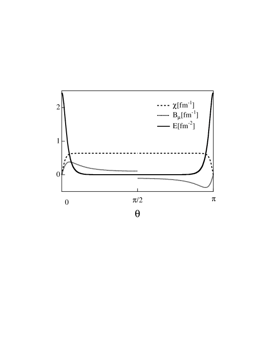
Figure 10.3: The color-electric field $E(\theta)$ (solid curve), the monopole condensate $\bar{\chi}(\theta)$ (dashed curve) and the dual gauge field $B(\theta)$ (dotted curve) are plotted as functions of the polar angle $\theta$ for the low density case with $R=$4.0fm.

Here, we consider the critical radius $R_{c}$ of the phase transition to the normal phase, where the monopole condensate disappears. There are three useful inequalities on $f_{E}$, $f_{\chi}$, and $F$,

$$f_{E}\geq 2\pi(\frac{n}{g})^{2}$$ (10.21)

$$0\leq f_{\chi}\leq\ 4\pi\lambda v^{4},$$ (10.22)

$$F=f_{0}+f_{E}\cdot\frac{1}{R^{2}}+f_{\chi}\cdot R^{2}\geq f_{0}+2\sqrt{f_{E}f_{\chi}}.$$ (10.23)

The equality is satisfied in Eq.(10.23),

$$R^{4}=\frac{f_{E}}{f_{\chi}}$$ (10.24)

Using the inequalities equations(10.21)-(10.23), $R^{4}$ is larger than the critical $R^{4}_{c}$;

$$R^{4}\geq R^{4}_{c}\equiv\frac{2\pi n^{2}/g^{2}}{4\pi\lambda v^{4}}=\large(\frac{n^{2}}{2\lambda g^{2}}\large)\frac{1}{v^{4}}.$$ (10.25)

For $R>R_{c}$, there exists a nontrivial inhomogeneous solution, which differs from the normal phase. For $R\leq R_{c}$, homogeneous normal phase provides the minimum of $F$. Thus, $R_{c}$ is the critical radius of the phase transition from the flux-tube phase to the normal one. In this case, the critical radius and the electric field are given by

$$\rho_{c}=\frac{1}{2\pi R^{2}_{c}}=\sqrt{\frac{\lambda}{2}}\frac{gv^{2}}{\pi n},$$ (10.26)

$$E_{c}=\frac{n}{gR_{c}^{2}}=\sqrt{2\lambda}v^{2},$$ (10.27)

respectively.

10.2 Numerical Results on Multi-flux-tube System

We start with showing the low density case of two flux tubes system in Fig.10.3. The parameters of the DGL theory are fixed as $\lambda=$ 25, $v=$ 0.126GeV, which lead the masses $m_{B}=$ 0.5GeV and $m_{\chi}=$ 1.26GeV [33]. This parameter set provides the flux-tube radius $r_{FT}\sim$0.4fm and the suitable interquark potential with the string tension as $\sigma=$1GeV/fm. The monopole condensate $\bar{\chi}(\theta)$, the dual gauge field $\tilde{B}(\theta)$ and the color electric field $E(\theta)$ are plotted as functions of the polar angle $\theta$. The electric field $E(\theta)$ is localized around the two poles($\theta$=0 and $\pi$) and drops suddenly as $\theta$ deviates from the two poles. The monopole condensate vanishes at the two poles and becomes constant in the region away from these poles. This behavior corresponds to the case of independent two vortices in superconductivity. Different from these physical quantities, the dual gauge field $\tilde{B}(\theta)$ is discontinuous at $\theta=\pi/2$. There should be Dirac-string like source to provide, because the electric flux leaving out from the two poles. It should be noted that the system has the reflection symmetry on $\theta=\frac{\pi}{2}$ plane.

We show now in Fig.10.4 the number density dependence of the flux-tubes. For the large radius of the sphere, ($R\geq$2fm), the color electric flux is localized at $\theta=0$ and $\pi$ and there the monopole condensate vanishes, while the $\bar{\chi}$ becomes constant $\bar{\chi}\simeq v$ around $\theta=\frac{\pi}{2}$. As the radius $R$ decreases, the electric flux, localized at $\theta=0$, $\theta=\pi$, starts to overlap, and the value of the monopole condensate $\bar{\chi}$ becomes small. The electric field $E(\theta)$ becomes constant and $\bar{\chi}$ vanishes below a critical radius $R_{c}$. We show in Fig.10.5 the monopole condensate at $\theta=\frac{\pi}{2}$ (the maximum value of the monopole condensate) as a function of the sphere radius $R$ (flux-tube number density $\rho=1/(2\pi R^{2})$). The (first order) phase transition occurs and the system becomes homogeneous normal phase above the critical value of the flux-tube number density.

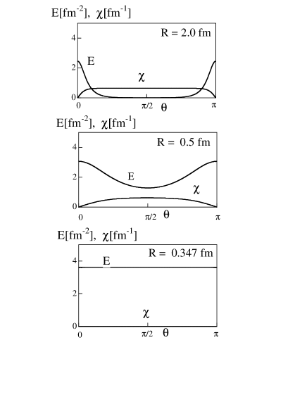
Figure 10.4: The flux-flux system on $S^{2}$. The color-electric field $E(\theta)$ and the monopole condensate $\bar{\chi}(\theta)$ are depicted as functions of the polar angle $\theta$ for the three radii; $R=$2.0fm, 0.5fm and 0.347fm. Below the critical radius $R_{c}$=0.347fm, the color-electric field $E$ becomes constant and the monopole condensate $\bar{\chi}$ vanishes entirely.

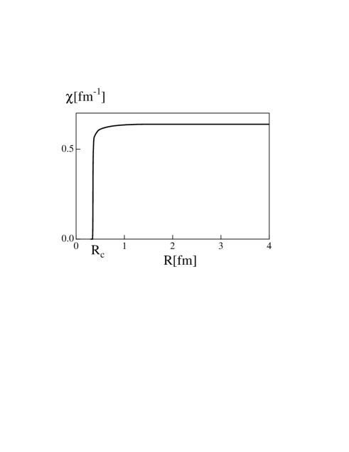
Figure 10.5: The $R$ dependence of the monopole condensate. Here, the flux tube density is given by $1/(2\pi R^{2})$. The monopole condensate at $\theta=\frac{\pi}{2}$ decreases, as the radius $R$ becomes smaller, and vanishes below $R=R_{c}$.

Here, we compare the free energy of two flux tube system with that of inhomogeneous system in Fig.10.6. At large $R$, the former is smaller and the system favors the existence of two flux tubes. As $R$ becomes smaller, the energy difference of the system becomes smaller. Two flux-tubes melt and the electric field are changed to be homogeneous below the critical radius $R_{c}=0.35$fm, which corresponds to the critical density $\rho_{c}=1/(2\pi R_{c}^{2})=1.3{\rm fm}^{-2}$. This critical density agrees with the analytic estimation in Eq.(10.26), $\rho_{c}=\sqrt{\frac{\lambda}{2}}\frac{gv^{2}}{\pi n}=1.3{\rm fm}^{-2}$.

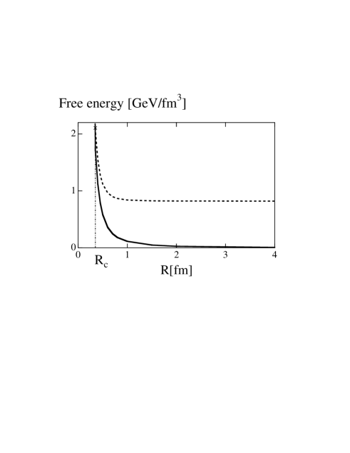
Figure 10.6: The free energy in flux-flux system (solid curve) and uniform system (dashed curve). Because the lower free energy system is realized, the inhomogeneous system is changed into a homogeneous system below the critical radius, $R_{c}=0.35{\rm fm}$. Here, the critical flux-tube density reads $\rho_{c}=1.3{\rm fm}^{-2}$.

We discuss now the system of flux-tube and anti-flux-tube with opposite direction placed at $\theta=$0 and $\theta=\pi$ respectively as shown in Fig.10.7. At low flux-tube number density ( $R\geq 2$fm), the flux-tube is localized at $\theta=0$, while the anti-flux-tube at $\theta=\pi$. The monopole condensate $\bar{\chi}(\theta)$ vanishes at the two poles ($\theta=0,\pi$) and becomes constant away from these poles. As $R$ decreases, the electric flux starts to cancel each other and the monopole condensate becomes small. We also compare the free-energy of the flux-tube and anti-flux-tube system with the homogeneous system, in which both monopole condensate and electric field are vanished. The critical radius, $R_{c}=$ 0.31fm, is similar to the value of the two flux-tubes system.

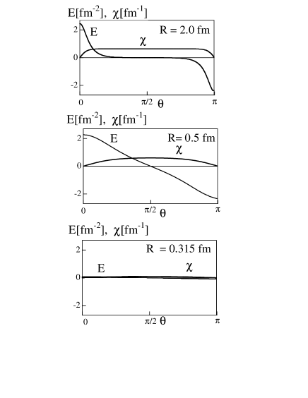
Figure 10.7: The flux the and anti-flux-tube system on $S^{2}$. The color-electric field $E(\theta)$ and the monopole condensate $\bar{\chi}(\theta)$ are depicted as functions of the polar angle $\theta$ for the three radii; $R=$2.0fm, 0.5fm, and 0.315fm. Below $R=$0.315fm, both the color electric flux and the monopole condensate vanish entirely.

Thus, we have found in both cases that the solution behaves as two independent flux-tubes at a large $R$, i.e., a small number density $\rho$. As the radius $R$ decreases, the monopole condensate decreases and eventually vanishes at a critical density, where the color-electric field $E$ becomes uniform. The critical density $\rho_{c}$ is found as $\rho_{c}=$1.3${\rm fm}^{-2}=(1.14{\rm fm})^{-2}$ for the two color-flux tube system; $\rho_{c}=$1.7${\rm fm}^{-2}=(1.3{\rm fm})^{-2}$ for the flux-tube and anti-flux-tube system. Such similar values in both cases suggest that an actual flux-tube system would become uniform around similar density to $\rho_{c}\sim$1.5fm^-2, because realistic flux-tube system includes the flux-tubes and anti-flux tubes randomly, which would correspond to an intermediate system between the above two ideal cases. Thus, the configuration of the color-electric field and the monopole field depend largely on the flux-tube density.

As discussed above, many flux-tubes are melted around $\rho_{c}\sim$ 1.5 fm^-2. Let us discuss here in case of central collision between heavy-ions with mass number $A$. The nuclear radius $R$ is given by $R=R_{0}A^{1/3}$, where $R_{0}$=1.2fm corresponds to the nuclear radius, and the normal baryon-number density is $\frac{A}{\frac{4}{3}\pi R^{3}}=\frac{1}{\frac{4}{3}\pi R_{0}^{3}}$. In the central region, one nucleon in the projectile makes hard collisions with $\frac{3}{2}A^{1/3}$$(=2\pi R_{0}^{3}A^{1/3}\times\rho_{0})$ nucleons in the target, because the reaction volume is $\pi R_{0}^{2}\times 2R=2\pi R^{3}_{0}A^{1/3}$. Hence, nucleon-nucleon collision number is expected as $(\frac{3}{2}A^{1/3})^{2}=\frac{9}{4}A^{2/3}$ per the single-nucleon area $\pi R_{0}^{2}$ between projectile and target nuclei. Assuming one flux-tube formed in one nucleon-nucleon hard collision, the flux-tube density is estimated as $\rho=\frac{\frac{9}{4}A^{2/3}}{\pi R_{0}^{2}}=\frac{A^{2/3}}{(1.4{\rm fm})^{2}}$. For instance, $\rho$ would be 4.5, 5.8 and 17.5 fm^-2 for $A=$ 27, 40 and 208. This would indicate that the scenario of creating large sizes of flux tube becomes much relevant for $A$-$A$ collision with larger $A$.

It would be important to reconsider the process of the QGP formation in terms of the flux-tube number density. When the flux-tube density is low enough, the flux-tubes are localized. Each flux-tube evolution would be regarded as the multi-creation of hadrons in the high energy p-p collision via the flux-tube breaking. In this process, $q$-$\bar{q}$ pair creation plays an essential role on the QGP formation, which is the usual scenario.

On the other hand, for the dense flux-tube system, neighboring flux-tubes are melted into a large cylindrical tube, where monopole condensate disappears. Such a system, where the color electric field is made between heavy-ions, becomes approximately homogeneous and is regarded as the ’color condenser’. In this case, large homogeneous QGP may be created in the central region.

In the actual case, however, the variations and directions of the color-flux-tubes are random. For instance, in the peripheral region, flux-tubes would be localized and are broken by quark-antiquark pair creations. In the central region, dense flux-tubes are melted by annihilation or unification [90] of flux-tubes, which will be discussed in the next section. In this region, a huge system of dynamical gluons appears, because many dynamical gluons are created during this process. Thermalization of such quarks and gluons leads to QGP. Thus, the process of QGP formation should depend largely on the density of created flux-tubes, which is closely related to the incident energy, the impact parameter and the size of the projectile and the target nuclei.

10.3 Flux-tube Interaction and QGP Formation Process

Finally, we investigate the interaction among various color-flux-tubes, which is considered to be important for the QGP formation process. Each flux tube is characterized by the color charge $\vec{Q}$ [69, 91] at its one end. To classify sorts of the flux tube, we call the flux tube with a red quark ($R$) at its one end as “$R$-$\bar{R}$ flux tube”, and so on. In this case, the “direction” of the color-electric flux in the flux tube should be distinguished. For instance, $\bar{R}$-$R$ flux tube is different from $R$-$\bar{R}$ flux tube in terms of the flux direction. We study the interaction between two color-electric flux tubes using the DGL theory. The color-electric charges at one end of the flux tubes are denoted by $\vec{Q}_{1}$ and $\vec{Q}_{2}$. We idealize the system as two sufficiently long flux tubes, and neglect the effect of their ends. We denote by $d$ as the distance between the two flux tubes. For $d\gg m_{\chi}^{-1}$, the interaction energy per unit length in the two flux tube system is estimated as

$$E_{\rm int}\simeq{8\pi\vec{Q}_{1}\cdot\vec{Q}_{2}\over e^{2}}m_{B}^{2}K_{0}(m_{B}d),$$ (10.28)

where $K_{0}(x)$ is the modified Bessel function. Here, we have used the similar calculation on the Abrikosov vortex in the type-II superconductor [93].

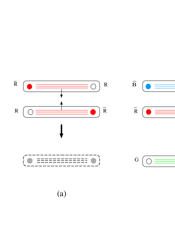
Figure 10.8: The annihilation process of the color-electric flux tubes during the QGP formation in ultrarelativistic heavy-ion collisions. (a) The same flux tubes with opposite flux direction are attracted each other, and are annihilated into dynamical gluons. (b) The different flux tubes (e.g. $R$-$\bar{R}$ and $B$-$\bar{B}$) are attractive, and are unified into a single flux tube.

As shown in Fig.10.8, there are two interesting cases on the interaction between two color-electric flux tubes.

1. (a) For the same flux tubes with opposite flux direction (e.g. $R$-$\bar{R}$ and $\bar{R}$-$R$), one finds $\vec{Q}_{1}=-\vec{Q}_{2}$ i.e. $\vec{Q}_{1}\cdot\vec{Q}_{2}=-e^{2}/3$, so that these flux tubes are attracted each other. It should be noted that they would be annihilated into dynamical gluons in this case.

2. (b) For the different flux tubes satisfying $\vec{Q}_{1}\cdot\vec{Q}_{2}<0$ (e.g. $R$-$\bar{R}$ and $B$-$\bar{B}$), one finds $\vec{Q}_{1}\cdot\vec{Q}_{2}=-e^{2}/6$, so that these flux tubes are attractive. In this case, they would be unified into a single flux tube (similar to $\bar{G}$-$G$ flux tube).

Based on the above calculation, we propose a new scenario on the QGP formation via the annihilation of the color-electric flux tubes. When the flux tubes are sufficiently dense in the central region just after ultrarelativistic heavy-ion collisions, many flux tubes are annihilated or unified. During the annihilation process of the flux tubes, lots of dynamical gluons (and quarks) would be created. Thus, the energy of the flux tubes turns into that of the stochastic kinetic motion of gluons (and quarks). The thermalization is achieved through the stochastic gluon self-interaction, and finally the hot QGP would be created. Here, the gluon self-interaction in QCD plays an essential role to the thermalization process, which is quite different from the photon system in QED.

In more realistic case, both the quark-pair creation and the flux-tube annihilation would take place at the same time. For instance, the flux tube breaking [89, 94, 95] would occur before the flux tube annihilation for the dilute flux tube system. On the contrary, in case of the extremely high energy collisions, these would be lots of flux tubes overlapping in the central region between heavy ions, and therefore the flux tube annihilation should play the dominant role in the QGP formation. In any case, the DGL theory would provide a calculable method for dynamics of the color-electric flux tubes in the QGP formation.

Chapter 11 Summary and Concluding Remarks

In the basis of the dual superconductor picture, we have systematically studied the confinement phenomena using the lattice QCD Monte-Carlo simulation, the monopole-current dynamics and the dual Ginzburg-Landau (DGL) theory, an infrared effective theory of QCD. In the dual Higgs theory, color confinement is understood by one-dimensional squeezing of the color-electric flux in the QCD vacuum through the dual Meissner effect caused by monopole condensation. For the construction of the dual superconducting theory from QCD, there are two large gaps on speciality of the abelian sector and the appearance of monopoles, however, these gaps are expected to be fulfilled by taking the ’t Hooft abelian gauge fixing, which is defined by the diagonalization of a suitable gauge-dependent variable, $\Phi[A_{\mu}(x)]$. In the abelian gauge, the SU($N_{c}$) gauge theory is reduced into the U(1)${}^{N_{c}-1}$ gauge theory including color-magnetic monopoles, which topologically appears corresponding to the nontrivial homotopy group, $\Pi_{2}($SU$(N_{c})/$U$(1)^{N_{c}-1})={\bf Z}^{N_{c}-1}$. In this gauge, the diagonal and the off-diagonal gluon components behave as the abelian gauge field and the charged matter field, respectively, in terms of the residual gauge symmetry. As a remarkable fact, “abelian dominance”, irrelevance of off-diagonal gluons, is numerically observed for the nonperturbative QCD phenomena like confinement and dynamical chiral-symmetry breaking in the lattice QCD simulation in the MA gauge, which is a sort of the abelian gauge. Monopole condensation has been also suggested by the lattice QCD as the appearance of the global network of the monopole current in the MA gauge.

First, we have studied the origin of abelian dominance for the confinement force in MA gauge in terms of the gluon-field properties using the lattice QCD. In the MA gauge, the gluon-field fluctuation is maximally concentrated in the abelian sector. As the remarkable feature in the MA gauge, we have found that the amplitude of the off-diagonal gluon is strongly suppressed, and therefore the phase variable of the off-diagonal (charged) gluon tends to be random, according to the weakness of the constraint from the QCD action. Using the random-variable approximation for the charged-gluon phase variable, we have found the perimeter law of the charged-gluon contribution to the Wilson loop and have proved abelian dominance for the string tension in the semi-analytical manner. These theoretical results have been also numerically confirmed using the lattice QCD simulation.

Second, we have studied th QCD-monopole appearing in the abelian sector in the abelian gauge. The appearance of monopoles have been transparently formulated in terms of the gauge connection, and is originated from the singular nonabelian gauge transformation to realize the abelian gauge. We have investigated the gluon field around the monopole in the lattice QCD. The QCD-monopole carries a large fluctuation of the gluon field and provides a large abelian action of QCD. Nevertheless, QCD-monopoles can appear in QCD without large cost of the QCD action, due the large cancellation between the abelian and off-diagonal parts of the QCD action density around the monopole. We have derived a simple relation between the confinement force and the monopole density by idealizing the monopole contribution to the Wilson loop.

Third, we have studied the monopole-current dynamics using the infrared monopole-current action defined on a lattice. We have adopted the local current action, considering the infrared screening of the inter-monopole interaction due to the dual Higgs mechanism. When the monopole self-energy $\alpha$ is smaller then $\alpha_{c}=$ ln$(2D-1)$, monopole condensation can be analytically shown, and we have found this system being the confinement phase from the Wilson loop analysis. By comparing the lattice QCD with the monopole-current system, the QCD vacuum has been found to corresponds to the monopole-condensed phase in the infrared scale. We have considered the derivation of the DGL theory from the monopole ensemble, which would be essence of the QCD vacuum in the MA gauge because of abelian dominance and monopole dominance.

In the second half part of this paper, we have studied the deconfinement phase transition and the hadron flux-tube system using the DGL theory. Deconfinement phase transition is one of the most interesting subject in the QCD phase transition both for ultra-relativistic heavy-ion collisions and for early universe. We have formulated the effective potential in the DGL theory, introducing the quadratic source term to study the QCD vacuum at finite temperatures. We have found the reduction of the monopole condensate at finite temperatures, and found a first-order deconfinement phase transition at the critical temperature $T_{C}\simeq$ 0.49GeV using the temperature-independent parameters. The monopole condensate vanishes and the broken dual gauge symmetry is restored above $T_{C}$. We have considered the temperature dependence of the monopole self-interaction noting $T_{C}=0.28$GeV as the lattice QCD simulation indicates. We have found a large reduction of the monopole self-interaction near the critical temperature. We have investigated the temperature dependence of the masses for the relevant mode like $m_{B}$ and $m_{\chi}$, and have found their large reduction near the critical temperature $T_{C}$: $m_{B},m_{\chi}\sim T_{C}$. We have calculated also the string tension at finite temperatures. The results agree with the lattice QCD data both in the variable $\lambda(T)$ and in the variable $v(T)$ cases. In particular, the glueball mass reduction at high temperatures would be an important ingredient in the QCD phase transition. In the pure gauge, there are only glueball excitations with the large mass ($\stackrel{{\scriptstyle>}}{{\sim}}$ 1GeV) at low temperatures, and therefore it seems unnatural that the QCD phase transition takes place at a small critical temperature, $T_{C}\simeq$ 0.28GeV. This problem would be explained by the large reduction of the glueball mass near the critical temperature as is demonstrated. In other words, this glueball-mass reduction may determine the magnitude of the critical temperature $T_{C}$ in the QCD phase transition.

Based on this effective potential at finite temperature, we have investigated the properties of hadron bubbles created in the early Universe and discussed the hadron bubble formation process. From numerical results, we can imagine how the QCD phase transition happens in the big bang scenario. (a) Slightly below $T_{\rm c}$, only large hadron bubbles appear, but the creation rate is quite small. (b) As temperature is lowered by the expansion of the Universe, smaller bubbles are created with much formation rate. During this process, the created hadron bubbles expand by radiating shock wave, which reheats the QGP phase around them.(c) Near $T_{\rm low}$, many small hadron bubbles are violently created in the unaffected region free from the shock wave. (d) The QGP phase pressed by the hadron phase is isolated as high-density QGP bubbles,which provide the baryon density fluctuation.Thus, the numerical simulation using the DGL theory would tell how the hadron bubbles appear and evolve quantitatively in the early Universe.

We have studied the multi-flux-tube system in terms of the DGL theory. We have considered two ideal cases, where the directions of all the color-flux-tubes are the same in one case and alternative in the other case for neighboring flux-tubes. We have formulated the system of multi color-flux-tubes by regarding it as the system of two color-flux-tubes penetrating through a two dimensional sphere surface. We have found the multi flux-tube configuration becomes uniform above some critical flux-tube number density $\rho_{c}=1.3\sim 1.7{\rm fm}^{-2}$. On the other hand, the inhomogeneity on the color electric distribution appears when the flux-tube density is smaller than $\rho_{c}$. We have discussed the relation between the inhomogeneity in the color-electric distribution and the flux-tube number density in the multi-flux-tube system created during the QGP formation process in the ultra-relativistic heavy-ion collision. When the flux-tube number density is low enough, the system can be approximated as the incoherent sum of the individual flux tube. Its evolution would lead to the creation of $q$-$\bar{q}$ pairs via flux-tube breaking. In this process, this $q$-$\bar{q}$ creation plays a essential role on the QGP formation. On the other hand, for a dense flux-tube system, neighboring flux tubes are melted into a large cylindrical tube, which is approximately homogeneous in the whole space and is regarded as the “color condenser”. In this case, large homogeneous QGP may be created in the central region. Thus, the process of QGP formation is expected depending largely on the density of created flux tubes. We have finally investigated also the interaction of two color-flux-tubes in the DGL theory and showed that there is a possibility of annihilation or unification of two color-flux-tubes when the flux tubes are sufficiently dense. This process would provide an enough energy to create many dynamical gluons and to form QGP.

Acknowledgment

We are grateful for useful discussions and supports with Professor H. Toki and all the members of the Research Center for Nuclear Physics theory group. Simulations were performed on VPP500 at RIKEN and SX4 at RCNP.

Appendix A Monte Carlo Method for Lattice QCD

A.1 Gauge Field on the Lattice

Quantum Chromodynamics (QCD), a nonabelian gauge theory, is difficult to solve analytically due to the large gauge coupling in the low-energy region. The Monte Carlo simulation based on the lattice gauge theory is one of the promising methods for the direct calculation of the QCD partition functional. We review here the fundamentals of the lattice QCD and the numerical simulation [69].

The Minskowski space-time is transformed into Euclidean space-time by replacing $x^{0}=-ix^{4}$, where $x^{0}$ and $x^{4}$ are the Minskowski and the Euclidean time, respectively. A similar transformation is made in the time component of all four-vectors. In the Euclidean space, there is no distinction between upper and lower indices of four-vector, i.e, $x_{\mu}^{\rm E}=(x^{1},x^{2},x^{3},x^{4})=(x_{1},x_{2},x_{3},x_{4})$.

In principle, to latticize the theory is performed by the replacement of derivatives by finite differences with the lattice spacing $a$. This method, however, does not preserve gauge invariance, which is an essential attribute of the theory. Wilson introduced a gauge-invariant lattice action using the path representation of the gauge group $G$. The most elementary paths on the lattice are links out of which any path can be constructed. The link is identified by the site $s$ and the direction $\mu$. With each link on the lattice, we associate a group element, called the “link variable” as

$$U_{\mu}(s)\equiv{\rm exp}\{iaeA_{\mu}(s)\}\equiv{\rm exp}\{i\theta_{\mu}(s)\}\hskip 14.22636pt\in G,$$ (A.1)

with the gauge coupling constant $e$. The lattice angle variables $\theta_{\mu}$ defined as $\theta_{\mu}\equiv\theta_{\mu}^{a}T^{a}\equiv aeA_{\mu}$ is dimensionless, and link variable $U_{\mu}(s)$ is transformed as

$$U_{\mu}(s)\rightarrow V(s)U_{\mu}(s)V^{\dagger}(s+\hat{\mu}),$$ (A.2)

where $V(s)$ and $V(s+\hat{\mu})$ are the gauge functions located at the starting and the end points of the link $U_{\mu}(s)$. Thus, the gauge transformation is described by simple multiplication of the group elements in the lattice formalism.

In the continuum, the field strength tensor $G_{\mu\nu}\equiv G_{\mu\nu}^{a}T^{a}\in{g}$ is defined in terms of an infinitesimal closed path. By analogy, we defined it on the lattice in terms of a “plaquette” $\Box_{\mu\nu}$, a square bounded by four links. The field tensor $G_{\mu\nu}$, which is associated with the oriented plaquette specified by the links $\{\mu,\nu\}$ attached to site $s$, is defined through the relation

$$\Box_{\mu\nu}(s)\equiv U_{\mu}(s)U_{\nu}(s+\hat{\mu})U^{\dagger}_{\mu}(s+\hat{\nu})U_{\nu}^{\dagger}(s)\equiv{\rm exp}(iea^{2}G_{\mu\nu}(s))\hskip 14.22636pt{\in G}.$$ (A.3)

For $a\rightarrow 0$, we recover the continuum field tensor,

$$G_{\mu\nu}(s)=\frac{1}{a}[(A_{\nu}(s+\hat{\mu})-A_{\nu}(s))-(A_{\mu}(s+\hat{\nu})-A_{\mu}(s))]+ie[A_{\mu}(s),A_{\nu}(s)]+O(a).$$

The lattice action is constructed by using the relation,

$$\sum_{s}\sum_{\mu,\nu}{\rm tr}\Box_{\mu\nu}(s)=\sum_{s}\sum_{\mu,\nu}{\rm tr}[1-iea^{2}G_{\mu\nu}-\frac{1}{2}e^{2}a^{4}(G_{\mu\nu})^{2}+\cdots],$$ (A.4)

where $\mu$ and $\nu$ are summed from 1 to 4. The first term on the right hand side is a constant, and the second term vanishes because $G_{\mu\nu}$ is traceless. The sum over $s$, $\mu$, $\nu$ on the left hand side is twice the sum over all plaquettes, so that one finds

$$\sum_{s}\sum_{\mu\neq\nu}{\rm tr}\Box_{\mu\nu}=\sum_{s}\sum_{\mu>\nu}({\rm tr}\Box_{\mu\nu}+{\rm tr}\Box_{\mu\nu}^{\dagger})=2{\rm Re}\sum_{s}\sum_{\mu>\nu}{\rm tr}\Box_{\mu\nu}.$$ (A.5)

Because interchanging $\mu$ and $\nu$ changes the orientation of the designated plaquette. Thus, we have

$$\sum_{s}\sum_{\mu>\nu}{\rm Re}\,\,{\rm tr}\Box_{\mu\nu}\rightarrow-\frac{1}{4}e^{2}\int d^{4}x\sum_{\mu,\nu}{\rm tr}(G_{\mu\nu})^{2}+{\rm const.},$$ (A.6)

as $a\rightarrow 0$. Here, the sum on the left hand side extends over all plaquettes on the lattice.

Finally, we get the lattice QCD action as

$$S = \int d^{4}x\sum_{\mu,\nu}\frac{1}{2}{\rm tr}(G_{\mu\nu})^{2}=\frac{2}{e^{2}}\sum_{s}\sum_{\mu>\nu}{\rm Re}\,{\rm tr}\left[1-\Box_{\mu\nu}(s)\right]$$ (A.7)

$$= \beta\sum_{s}\sum_{\mu>\nu}{\rm Re}\,\frac{1}{N_{c}}{\rm tr}\left[1-\Box_{\mu\nu}(s)\right],$$

where $\beta\equiv\frac{2N_{c}}{e^{2}}$ is the control parameter relating to the lattice spacing $a$. The continuum limit $a\rightarrow 0$ corresponds to $e\rightarrow 0$ or $\beta\rightarrow\infty$ in the theory with the asymptotic freedom like QCD. Thus, the QCD partition functional in the lattice formalism is given as

$$Z=\int dU_{\mu}e^{-S[U_{\mu}(s)]}=\int[\Pi_{s,\mu}dU_{\mu}(s)]e^{-S[U_{\mu}(s)]}.$$ (A.8)

For SU(2), the link variable $U_{\mu}(s)$ is parameterized as $U_{\mu}\equiv U_{\mu}^{0}+i\tau^{a}U_{\mu}^{a}$, and the measure takes a form

$$dU_{\mu}(s)\equiv dU_{\mu}^{0}dU_{\mu}^{1}dU_{\mu}^{2}dU_{\mu}^{3}\delta(U_{0}^{2}+U_{1}^{2}+U_{3}^{2}+U_{3}^{2}-1).$$ (A.9)

The expectation value of arbitrary operator $O$ is calculable as

$$\langle O\rangle\equiv\frac{\int dU_{\mu}Oe^{-S[U_{\mu}]}}{\int dU_{\mu}e^{-S[U_{\mu}]}}$$ (A.10)

using the numerical simulation with the Monte Carlo method.

A.2 Monte Carlo Method

In this section, we briefly summarized the Monte Carlo method of the lattice QCD. In the lattice QCD with the action (A.7), the ensemble of gauge configuration is given by the canonical ensemble, characterized by Boltzmann distribution,

$$P(U)=\frac{1}{Z}e^{-\beta\hat{S}},$$ (A.11)

where we put $S[U]=\beta\hat{S}[U]$ and regard $\hat{S}[U]$ as a “Hamiltonian”. In principle, the lattice QCD partition function $Z$ can be calculated by the infinite number of Monte Carlo simulations using any random sampling of $U_{\mu}$. In practical, however, almost all gauge configurations with large $\hat{S}$ do not contribute to the lattice QCD partition functional $Z$. Therefore, it is necessary to sample the “important gauge configuration” with small $\hat{S}$ effectively in terms of the numerical calculation with finite number of operations. Such a “important sampling” can be realized by generating the random number with the weight $e^{-\beta\hat{S}[U]}$, and the Monte Carlo method enables us to calculate the lattice QCD partition function, numerically.

In the Monte Carlo method, our goal is to generate a time sequence of configurations such that the configuration $U$ occurs with probability $P(U)$ after a sufficiently long time. Thus, the time average of any quantity would be the same as its average over the canonical ensemble.

The time sequence is generated by a stochastic process. A configuration $U$ is updated to $U^{\prime}$ with a transition probability $T(U^{\prime},U)$, which has the following general properties:

1. $T(U^{\prime},U)\geq 0$

2. $\int dU^{\prime}T(U^{\prime},U)=\int dUT(U,U^{\prime})=1$,

3. $T(U^{\prime},U)P(U)dU=T(U,U^{\prime})P(U^{\prime})dU^{\prime}$.

The first two are just properties that any probability should have. The last is known as the condition of detailed balance. Integrating over $U^{\prime}$ on both sides of the last condition, we obtain

$$P(U)=\int dU^{\prime}T(U,U^{\prime})P(U^{\prime}),$$ (A.12)

which states that the probability $P(U)$ is an eigenfunction of $T(U^{\prime},U)$. This means that transition probability preserves the equilibrium ensemble. Thus, we get the gauge configuration ensemble obeying $P(U)$ as a “time” sequence of “thermalization”. Using the obtained gauge configuration, the ensemble average of arbitrary operator $O(U)$ is numerically estimated by

$$\langle O\rangle=\int dUO(U)P(U).$$ (A.13)

On the actual numerical simulation, there are two cautions to be carefully checked. One is the achievement of the thermo-equilibrium, the other is the vanishing of the cancellation among the sampling gauge configurations.

Appendix B Procedure of Maximally Abelian Gauge Fixing

The maximally abelian (MA) gauge is the special abelian gauge exhibiting infrared abelian dominance in the lattice QCD, and provides the theoretical basis of dual Higgs picture from QCD. In the SU(2) lattice formalism, the MA gauge is defined so as to maximize

$$R_{\rm MA}[U_{\mu}] \equiv \frac{1}{2}\sum_{s}R(s)$$ (B.1)

$$\equiv \sum_{s,\mu}{\rm tr}\{U_{\mu}(s)\tau_{3}U^{\dagger}_{\mu}(s)\tau_{3}\}$$

$$= 2\sum_{s,\mu}\{U^{0}_{\mu}(s)^{2}+U^{3}_{\mu}(s)^{2}-U^{1}_{\mu}(s)^{2}-U^{2}_{\mu}(s)^{2}\}$$

$$= 2\sum_{s,\mu}\left[1-2\{U^{1}_{\mu}(s)^{2}+U^{2}_{\mu}(s)^{2}\}\right]$$

by the gauge transformation. Here, $R(s)$ is a local scalar variable defined as

$$R(s)\equiv\sum_{\pm\mu}{\rm tr}\{U_{\pm\mu}(s)\tau_{3}U^{\dagger}_{\pm\mu}(s)\tau_{3}\}\hskip 28.45274pt\mbox{with}\hskip 28.45274ptU_{-\mu}(s)=U^{\dagger}_{\mu}(s-\mu).$$ (B.2)

Here, $R(s)$ is manifestly invariant under the lattice rotation and the reflection. In the MA gauge, the operator

$$\Phi(s)\equiv\sum_{\mu,\pm}U_{\pm\mu}(s)\tau_{3}U^{\dagger}_{\pm\mu}(s)$$ (B.3)

is diagonalized. In this appendix, we show the procedure of the MA gauge fixing on the lattice.

To begin with, we introduce a “local” gauge transformation, whose gauge function $V_{s_{0}}(s)$ is not unity at the site $s_{0}$ only,

$$\left\{\begin{array}[]{llll}V_{s_{0}}(s)&=&V(s_{0})&\hskip 28.45274pt\mbox{for $s=s_{0}$}\\ V_{s_{0}}(s)&=&1&\hskip 28.45274pt\mbox{for $s\neq s_{0}$}.\end{array}\right.$$ (B.6)

In order to maximize the value $R_{\rm MA}[U_{\mu}]$, one may consider to maximize the local variables $R(s)$ at each site $s$ by the local gauge transformation $V_{s}$. However, since $R(s_{0})$ at the site $s_{0}$ is changed not only by the gauge transformation $V_{s_{0}}(s)$ but also by the gauge transformation $V_{s_{0}-\hat{\mu}}(s)$ with neighboring sites $s_{0}-\hat{\mu}$, one cannot obtain the MA gauge configuration $U_{\mu}(s_{0})^{\rm MA}$ only by simple local gauge transformation $V_{s_{0}}(s)$. After the local gauge transformation at all sites on the whole lattice, one has to repeat this procedure until $R_{\rm MA}$ is maximized.

Now, let us derive the gauge transformation $V_{s_{0}}(s)$ to maximize $R(s_{0})$. After the gauge transformation by $V_{s_{0}}(s)$, $R(s_{0})$ is changed as

$$R^{V}(s_{0}) = \sum_{\mu}{\rm tr}\{V(s_{0})U_{\mu}(s_{0})\tau_{3}U^{\dagger}_{\mu}(s_{0})V^{\dagger}(s_{0})\tau_{3}$$ (B.7)

$$+U_{\mu}(s_{0}-\hat{\mu})V^{\dagger}(s_{0})\tau_{3}V(s_{0})U^{\dagger}(s_{0}-\hat{\mu})\tau_{3}\}$$

$$= {\rm tr}[\sum_{\mu}\{U_{\mu}(s_{0})\tau_{3}U^{\dagger}(s_{0})+U^{\dagger}_{\mu}(s_{0}-\hat{\mu})\tau_{3}U_{\mu}(s_{0}-\hat{\mu})\}\cdot V^{\dagger}(s_{0})\tau_{3}V(s_{0})]$$

$$\equiv {\rm tr}[\Phi(s_{0})S(s_{0})].$$

Here, we define

$$S(s)\equiv S^{a}(s)\tau^{a}\equiv\vec{S}\cdot\vec{\tau}\equiv V^{\dagger}(s)\tau_{3}V(s)\hskip 28.45274pt\in\mbox{ su(2)},$$ (B.8)

$$\Phi(s)\equiv\Phi^{a}(s)\tau^{a}\equiv\vec{\Phi}\cdot\vec{\tau}\equiv\sum_{\pm\mu}U_{\pm\mu}(s)\tau_{3}U^{\dagger}_{\pm\mu}(s)\hskip 28.45274pt\in\mbox{su(2)},$$ (B.9)

which are both elements of Lie algebra and satisfy relations tr$(\Phi)=$ tr$(S)=0$ and $S^{2}=1$. To maximize $R(s_{0})$ by this gauge transformation, $\vec{S}(s_{0})$ is taken to be the same direction as $\vec{\Phi}(s_{0})$ in the SU(2) $\simeq$ O(3) parameter space, $\vec{S}//\vec{\Phi}$. After this gauge transformation, $\Phi(s_{0})$ is diagonalized as $\Phi^{V}(s_{0})=V(s_{0})\Phi(s_{0})V^{\dagger}(s_{0})=\Phi^{V}_{3}(s_{0})\tau_{3}$, and $S(s_{0})$ becomes $\tau_{3}$. Here, $\Phi$ plays a similar role as the Higgs field in the ’t Hooft-Polyakov monopole.

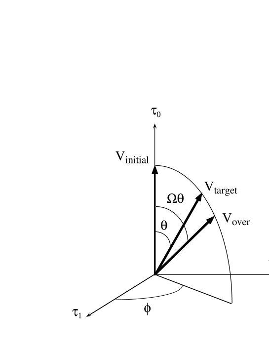
Figure B.1: The gauge function $\vec{V}_{\rm over}$ used in the over-relaxation method. The vector $\vec{V}_{\rm target}$ corresponds to the gauge function which maximizes $R(s_{0})$.

In the abelian gauge, the gauge function $V(s)$ is an element of the coset space SU(2)/U(1)₃ using the residual U(1)₃ degrees of freedom. We take the representative element of $V(s)$ so as to satisfy $V^{3}(s)=0$, or

$$V(s)=V^{0}(s)+i\{V^{1}(s)\tau^{1}+V^{2}(s)\tau^{2}\}.$$ (B.10)

Because of $(V^{1})^{2}+(V^{2})^{2}+(V^{3})^{2}=1,$ we can parameterize $V(s)$ as

$$\left\{\begin{array}[]{lll}V^{0}(s)&=&\cos\theta(s)\\ V^{1}(s)&=&\sin\theta(s)\cos\phi(s)\\ V^{2}(s)&=&\sin\theta(s)\sin\phi(s),\end{array}\right.$$ (B.14)

and then $S(s)$ is expressed as

$$S\equiv S^{a}\tau^{a}\equiv V^{\dagger}\tau_{3}V=\sin 2\theta\cos\phi\tau_{1}+\sin 2\theta\sin\phi\tau_{2}+\cos 2\theta\tau_{3}.$$ (B.15)

Since $\Phi(s_{0})\equiv\Phi^{a}(s_{0})\tau^{a}$ is obtained from the original gauge configuration $U_{\mu}(s)$, we get $V_{s_{0}}(s_{0})$ as

$$\left\{\begin{array}[]{lll}\tan^{2}2\theta(s_{0})&=&\frac{(S^{1})^{2}+(S^{2})^{2}}{(S^{3})^{2}}=\frac{(\Phi^{1})^{2}+(\Phi^{2})^{2}}{(\Phi^{3})^{2}}\\ \tan\phi(s_{0})&=&\frac{S^{2}}{S^{1}}=\frac{\Phi^{2}}{\Phi^{1}}.\end{array}\right.$$ (B.18)

Thus, the gauge function $V(s)$ which maximizes $R(s_{0})$ is obtained so as to obey $\vec{S}(s_{0})//\vec{\Phi}(s_{0})$. This procedure makes $R(s_{0})$ defined in (B.7) maximum by $V_{s_{0}}(s)$. This gauge transformation, however, influences $R(s)$ of the neighboring sites, $s=s_{0}\pm\hat{\mu}$, and in fact does not make them maximum. Therefore, we have to perform this procedure to the neighboring sites. By doing this, however, the original $R(s_{0})$ gets some change and hence $R(s_{0})$ is no more in its maximum. This fact forces us to repeat the local-gauge transformation many times.

To optimize the convergence, in the practical simulation, we take an over-relaxation method. We show the vector $(\cos\theta,\sin\theta\cos\phi,\sin\theta\sin\phi)$ in Fig.B.1, corresponding to the gauge function $V(s_{0})$ in Eq.(B.14). In the over-relaxation method, we take the angle value $\Omega\theta$ instead of $\theta$ obtained in Eq.(B.14),

$$\left\{\begin{array}[]{lll}V^{0}_{\rm over}(s_{0})&=&\cos(\Omega\theta)\\ V^{1}_{\rm over}(s_{0})&=&\sin(\Omega\theta)\cos\phi\\ V^{2}_{\rm over}(s_{0})&=&\sin(\Omega\theta)\sin\phi.\end{array}\right.$$ (B.22)

This overrelaxation parameter $\Omega$ is taken as $1\sim 2$.

Bibliography

- [1] For instance, T. P. Cheng and L. F. Li, “Gauge Theory of Elementary Particle Physics”, (Clarendon press, Oxford, 1984) 1.
- [2] O. Nachtmann, “Elementary Particle Physics”, (Springer, 1990) 1.
- [3] W. Greiner and A. Schafer, “Quantum Chromodynamics”, (Springer,1994) 1.
- [4] Y. Nambu and G. Jona-Lasinio, Phys. Rev.122 (1961) 345; 124 (1961) 246.
- [5] K. Higashijima, Prog. Theor. Phys. Suppl. 104 (1991) 1.
- [6] V. A. Miransky, “Dynamical Symmetry Breaking in Quantum Field Theories” (World Scientific, 1993) 1.
- [7] M. Shifman, “Instantons in Gauge Theories” (World Scientific, 1994) 1, and references therein.
- [8] R. Rajaraman, “Solitons and Instantons” (North-Holland, Amsterdam, 1982) 1.
-
[9]
D. I. Diakonov and V. Yu. Petrov, Nucl. Phys. B272 (1986)
457.
E. V. Shuryak, Phys. Rep. 115 (1984) 151. - [10] M. Bando, T. Kugo and K. Yamawaki, Phys. Rept. 164 (1988) 217.
- [11] A. W. Thomas, Adv. Nucl. Phys. 13 (1984) 1.
- [12] A. Hosaka and H. Toki, Phys. Rept. 277 (1996) 65.
- [13] S. P. Klevansky, Rev. Mod. Phys. 64 (1992) 649.
- [14] T. Hatsuda and T. Kunihiro, Phys Rept. 247 (1994) 221.
- [15] Y. Nambu, Phys. Rev. D10 (1974) 4262.
- [16] G. ’t Hooft, “High Energy Physics”, ed. A. Zichichi (Editorice Compositori, Bologna, 1975).
- [17] S. Mandelstam, Phys. Rep. C23 (1976) 245.
-
[18]
Y. Peng and R. W. Haymaker, Nucl. Phys. B (Proc. Suppl.) 34 (1996)
266.
R. W. Haymaker, V. Singh, Y. Peng and J. Wosiek, Phys. Rev.D53 (1996) 389. - [19] G. ’t Hooft, Nucl. Phys. B190 (1981) 455.
- [20] Z. F. Ezawa and A. Iwazaki, Phys. Rev. D25 (1982) 2681; D26 (1982) 631.
- [21] J. M. Kosterlitz and D. J. Thouless, J. Phys. C6 (1973) 1181.
-
[22]
S. Maedan and T. Suzuki, Prog. Theor. Phys. 81 (1989) 229.
T. Suzuki, Prog. Theor. Phys. 80 (1988) 929; 81 (1989) 752.
S. Maedan, Y. Matsubara and T. Suzuki, Prog. Theor. Phys. 84 (1990) 130. -
[23]
A. S. Kronfeld, G. Schierholz and U.-J. Wiese, Nucl. Phys. B293
(1987) 461.
A. S. Kronfeld, M. L. Laursen, G. Schierholz and U. -J. Wiese, Phys. Lett. 198B (1987) 516. - [24] F. Brandstater, U. J. Wiese and G. Schierholz, Phys. Lett. B272 (1991) 319.
- [25] T. Suzuki and I. Yotsuyanagi, Phys. Rev. D42 (1990) 4257; Nucl. Phys. B (Proc. Suppl.) 20 (1991) 236,
-
[26]
S. Hioki, S. Kitahara, S. Kiura, Y. Matsubara,
O. Miyamura, S. Ohno and T. Suzuki,
Phys. Lett. B272 (1991) 326.
S. Hioki, S. Kitahara, S. Ohno, T. Suzuki, Y. Matsubara and O. Miyamura, Phys. Lett. B285 (1992) 343. - [27] H. Ichie and H. Suganuma, Nucl. Phys. B (1999) in press, hep-lat/9807025; Phys. Rev. D (1999) in press.
-
[28]
O. Miyamura, Phys. Lett. B353 (1995) 91;
Nucl. Phys. B (Proc. Suppl.) 42 (1995) 538.
O. Miyamura and S. Origuchi, “Confinement ’95”, (World Scientific, 1995) 65. -
[29]
R. M. Woloshyn, Phys. Rev. D51 (1995) 6411.
F. X. Lee, R. M. Woloshyn and H. D. Trottier, Phys. Rev. D53 (1996) 1532. - [30] G. S. Bali, V. Bornyakov, M. Muller-Preussker and K. Schilling, Phys. Rev. D54 (1996) 2863.
- [31] A. Di Giacomo, Nucl. Phys. B (Proc. Suppl.) 47 (1996) 136 and references therein.
- [32] M. I. Polikarpov, Nucl. Phys. B (Proc. Suppl.) 53 (1997) 134 and references therein.
- [33] H. Suganuma, S. Sasaki and H. Toki, Nucl. Phys. B435 (1995) 207.
-
[34]
S. Sasaki, H. Suganuma and H. Toki,
Prog. Theor. Phys. 94 (1995) 373.
H. Suganuma, S. Umisedo, S. Sasaki, H. Toki and O. Miyamura, Aust. J. Phys. 50 (1997) 233. - [35] S. Umisedo, H. Suganuma and H. Toki, Phys. Rev.D57 (1998) 1605.
-
[36]
S. Thurner, M. C. Feurstein and H. Markum,
Phys. Rev. D56 (1997) 4039.
M. Feurstein, H. Markum and S. Thurner, Phys. Lett. B396 (1997) 203. - [37] H. Suganuma, K. Itakura and H. Toki, preprint, hep-th/9512141.
- [38] H. Suganuma, S. Sasaki, H. Ichie, F. Araki and O. Miyamura, Nucl. Phys. B (Proc. Suppl.) 53 (1997) 528.
-
[39]
M. Fukushima, S. Sasaki, H. Suganuma, A. Tanaka, H. Toki and D. Diakonov,
Phys. Lett. B399 (1997) 141,
M. Fukushima, A. Tanaka, S. Sasaki, H. Suganuma, H. Toki and D. Diakonov, Nucl. Phys. B (Proc. Suppl.) 53 (1997) 494.
M. Fukushima, H. Suganuma and H. Toki, preprint, hep-lat/9902005. - [40] R. C. Brower, K. N. Orginos and C. I. Tan, Phys. Rev. D55 (1997) 6313; Nucl. Phys. B (Proc. Suppl.) 53 (1997) 488.
- [41] S. Sasaki and O. Miyamura, Phys. Rev. D59 (1999) 94507; Phys. Lett. B443 (1998) 331.
- [42] H. J. Rothe, ”Lattice Gauge Theories”, (World Scientific, 1992) 1.
- [43] M. Creutz, ”Quarks, Gluons and Lattices” (Cambridge, 1983) 1.
- [44] K.-I. Kondo, Phys. Rev. D57 (1998) 7467; D58 (1998) 105016.
- [45] H. Ichie and H. Suganuma, preprint, hep-lat/9808054.
- [46] H. Suganuma, M. Fukushima, H. Ichie and A. Tanaka, Nucl. Phys. B (Proc. Suppl.) 65 (1998) 29.
-
[47]
H. Ichie, H. Suganuma and H. Toki, Phys. Rev. D52 (1995) 2994.
H. Monden, H. Ichie, H. Suganuma and H. Toki, Phys. Rev. C57 (1998) 2564. - [48] K. Amemiya and H. Suganuma, Proc. of Int. Symp. on “Innovative Computational Methods in Nuclear Many-Body Problems”, Osaka, Nov. 1997, (World Scientific),hep-lat/9712028; hep-lat/9811035.
- [49] H. Suganuma, H. Ichie, A. Tanaka and K. Amemiya, Prog. Theor. Phys. Suppl. 131 (1998) 559 and references therein.
- [50] G. I. Poulis, Phys. Rev. D54 (1996) 6974.
- [51] H. Ichie and H. Suganuma, Proc. of Int. Workshop on “Future Directions in Quark Nuclear Physics”, Adelaide, Australia, Mar. 1998, (World Scientific) in press, hep-lat/9807006.
- [52] H. Georgi, “Lie Algebras in Particle Physics”, (Benjamin/Cummings, 1982) 1.
- [53] J. E. Mandula and M. Ogilvie, Phys. Lett. B185 (1987) 127.
- [54] T. DeGrand and D. Toussaint, Phys. Rev. D22 (1980) 2478.
- [55] H. Ichie and H. Suganuma, Proc. of Int. Symp. on “Innovative Computational Methods in Nuclear Many-Body Problems”, Osaka, Nov. 1997, (World Scientific) 278, hep-lat/9802032.
-
[56]
J. D. Stack, Nucl. Phys. B (Proc. Suppl.) 34 (1994) 204.
J. D. Stack and R. J. Wensley and S. D. Neiman, Phys. Rev.D50 (1994) 3399. - [57] A. Tanaka and H. Suganuma, Proc. of Int. Symp. on “Innovative Computational Methods in Nuclear Many-Body Problems”, Osaka, Nov. 1997, (World Scientific),hep-lat/9712027; hep-lat/9901022.
- [58] H. Ichie and H. Suganuma, Proc. of INSAM Symp. ’96, Hiroshima, INSAM report, hep-lat/9709109.
- [59] H. Ichie, H. Suganuma and A. Tanaka, Nucl. Phys. B (Proc. Suppl.) 63A-C (1998) 468.
- [60] J. D. Stack, Nucl. Phys. B (Proc. Suppl.) 53 (1997) 524.
- [61] F. Brandstater, U.-J. Wiese and G. Schierholz, Phys. Lett. B272 (1991) 319-325.
- [62] A. Bode, T. Lipper and K. Schilling, Nucl. Phys. B (Proc. Suppl.) 34 (1994) 549.
- [63] S. Sasaki, Doctor thesis, Osaka University, 1997.
- [64] D. Zwanziger, Phys. Rev. D3 (1971) 880.
- [65] M. Blagojevic and P. Senjanovic, Nucl. Phys. B161 (1979) 112.
-
[66]
M. Stone and P. R. Thomas, Phys. Rev. Lett.41 (1978) 351.
P. R. Carlo and M. Stone, Nucl. Phys. B144 (1978) 513. - [67] K. Bardakci and S. Samuel, Phys. Rev. D18 (1978) 2849.
- [68] N. Nagaosa, “Quantum Field Theory”(in Japanese), (Iwanami, 1995) 1.
- [69] K. Huang, “Quarks, Leptons and Gauge Fields”, (World Scientific, Singapore, 1982) 1.
- [70] H. B. Nielsen and P. Olesen, Nucl. Phys. B61 (1973) 45.
-
[71]
For a review article,
W. Lucha, F. F. Schöberl and D. Gromes, Phys. Rep. 200 (1991) 127. - [72] H. Suganuma, S Sasaki, H. Ichie and F. Araki and O. Miyamura, Proc. of Int. Conf. on “Nuclear Physics Frontiers with Electroweak Probes”, Osaka, Japan, (World Scientific, 1996) 177.
- [73] H. Suganuma, S. Sasaki and H. Toki, Proc. of Int. Conf. on “Quark Confinement and Hadron Spectrum”, Como, Italy, (World Scientific, 1995) 241.
- [74] C. Itzykson and J.-B. Zuber, “Quantum Field Theory”, (McGraw-Hill, New York, 1985) 1.
- [75] H. Suganuma, H. Ichie, S. Sasaki and H. Toki, “Confinement ’95”, (World Scientific, 1995) 65.
-
[76]
G. Boyd, J. Engels, F. Karsch, E. Laermann,
C. Legeland, M. Lutgemeier and B. Petersson,
Phys. Rev. Lett. 75 (1995) 4169.
J. Fingberg, F. Karsch and U. M. Heller, Nucl. Phys. B (Proc. Suppl.) 30 (1993) 343. -
[77]
Y. Iwasaki, K. Kanaya, S. Sakai, T. Yoshie,
Nucl. Phys. B (Proc. Suppl.) 26 (1992) 311.
K. Kanaya, Prog. Theor. Phys. Suppl. 120 (1995) 25. - [78] H. Ichie, H. Monden, H. Suganuma and H. Toki, Proc. of Int. Symp. on “Nuclear Reaction Dynamics of Nucleon-Hadron Many Body System”, Osaka, Dec. 1995, (World Scientific, 1996) 246.
- [79] H. B. Nielsen and A. Patkos, Nucl. Phys. B195 (1982) 137.
- [80] For a review article, J. I. Kapusta, “Finite-Temperature Field Theory”, (Cambridge University Press, Cambridge, 1988) 1.
- [81] P. Ring and P. Schuck, “The Nuclear Many-Body Problem”, (Springer-Verlag, New York, 1980) 1.
- [82] H. Monden, T. Suzuki and Y. Matsubara, Phys. Lett. B294 (1992) 100.
- [83] J. Engels, F. Karsch, H. Satz and I. Montvay, Phys. Lett. B102 (1981) 332.
- [84] M. Gao, Nucl. Phys. B (Proc. Suppl.) 9 (1988) 368.
- [85] E. Witten, Phys. Rev. D30 (1984) 272.
- [86] T. Kajino, Proc. of Int. Symp. on “Nuclear Reaction Dynamics of Nucleon-Hadron Many Body System”, Osaka, Dec. 1995, (World Scientific, 1996) 231.
- [87] G. M. Fuller, G. J. Mathews and C. R. Alcock, Phys. Rev. D 37 (1988) 1380.
- [88] J. D. Bjorken, Phys. Rev. D27 (1983) 140.
- [89] N. K. Glendenning and T. Matsui, Phys. Rev. D28 (1983) 2890; Phys. Lett. B141 (1984) 419.
-
[90]
H. Ichie, H. Suganuma and H. Toki, Phys. Rev. D54 (1996) 3382.
Y. Koma, H. Suganuma and H. Toki, preprint, hep-ph/9902441. - [91] H. Suganuma, H. Toki, S. Sasaki and H. Ichie, Prog. Theor. Phys. Suppl. 120 (1995) 57.
- [92] N. S. Manton, Commun. Math. Phys. 111 (1987) 469.
- [93] E. M. Lifshitz and L. P. Pitaevsii, Vol.9 of Course of Theoretical Physics, “Statistical Physics, Part 2”, (Pergamon press, Oxford, 1981) 1.
- [94] G. Gatoff, A. K. Kerman and T. Matsui, Phys. Rev. D36 (1987) 114.
- [95] H. Suganuma and T. Tatsumi, Phys. Lett. B269 (1991) 371; Prog. Theor. Phys. 90 (1993) 379.