General Physics Motivations for Numerical Simulations of Quantum Field Theory

Abstract

In this introductory article a brief description of Quantum Field Theories (QFT) is presented with emphasis on the distinction between strongly and weakly coupled theories. A case is made for using numerical simulations to solve QCD, the regnant theory describing the interactions between quarks and gluons. I present an overview of what these calculations involve, why they are hard, and why they are tailor made for parallel computers. Finally, I try to communicate the excitement amongst the practitioners by giving examples of the quantities we will be able to calculate to within a few percent accuracy in the next five years.

LAUR-99-789

1 Introduction

The complexity of physical problems increases with the number of degrees of freedom, and with the details of the interactions between them. This increase in the number of degrees of freedom introduces the notion of a very large range of length scales. A simple illustration is water in the oceans. The basic degrees of freedom are the water molecules ($\sim 10^{-8}$ cm), and the largest scale is the earth’s diameter ($\sim 10^{4}$ km), $i.e.$ the range of scales span $10^{17}$ orders of magnitude. Waves in the ocean cover the range from centimeters, to meters, to currents that persist for thousands of kilometers, and finally to tides that are global in extent. Solutions to modeling the behavior of ocean waves depends on whether this whole range of scales are important or whether one can isolate them. For example, to understand the currents and tides one does not need to know the molecular nature of water at all, one can treat it as a continuous fluid. In general, different techniques are necessary depending on whether disparate length scales are strongly or weakly coupled.

The study of interactions between elementary particles involves length scales ($<10^{-13}$ cm ) where quantum effects are large. The quantum vacuum is no longer a smooth placid entity, but more like a frothing bubbling pot of stew. It has fluctuations at all scales from $10^{-13}$ cm to zero. The mathematical framework developed over the last fifty years for handling these fluctuations at all length scale is called Quantum Field Theory (QFT). (For a background on QFT see the text books [1].) Once again, the techniques used for solving these theories depend on how strongly these vacuum fluctuations couple to elementary processes like the scattering of two particles. These ideas are developed in Section 2. The coupling between quarks and gluons, the strongly interacting elementary particles, is $O(1)$ at the hadronic scale $10^{-13}$ cm. The associated QFT, called Quantum Chromodynamics (QCD), therefore involves both an infinite range of energy scales and a strong coupling. Thus, to answer many interesting questions like how neutrons and protons arise as bound states of quarks and gluons necessitates techniques different from the usual $--$ series expansion in a small coupling, $i.e.$ perturbation theory. The set of articles in this book explore the technique based on the numerical simulations of the underlying QFT discretized on a finite space-time grid. This brute force approach is the only known technique that is in principle exact. The remainder of this article is an attempt to show how the power of today’s supercomputers, especially massively parallel computers, can be used to solve this highly non-linear, strongly interacting QFT.

2 What is Quantum Field Theory

A pervasive feature of collisions between very high energy particles is the lack of conservation of the number of particles. The annihilation of an electron and positron, say each of energy 1 TeV in the center of mass, produces, in general, hundreds of particles (electrons, positrons, muons, pions, $etc.$). Thus, a theory of such interactions has to allow for the possibility of the spontaneous creation and annihilation of the various particles observed in nature. Such a theory should also obey the rules of quantum mechanics and relativity (Lorentz invariance). Quantum field theories have been remarkably successful in explaining three of the four forces: strong (QCD), electromagnetic(QED), and weak(WI). The effort of high energy physicists today is to develop techniques to extract very precise predictions of these theories and to confront these against results of experiments to determine if the theories are complete. The set of articles in this book explore a technique based on numerical simulations of QFT. Other physicists are trying to incorporate gravitational interactions, for which QFT has not been very successful, into our overall understanding. This effort has lead to exciting developments in string/M theory, however the discussion of these is beyond the scope of this article.

In QFT, the basic degrees of freedom are fields of operators defined at each and every space time point. These variables satisfy appropriate commutation/anti-commutation relations depending on their spin. Particles emerge as excitations of these field variables, and can be annihilated and created at any point. In fact there is a fundamental duality between the description of nature in terms of particles or fields. The interactions between the fields is local, $i.e.$ the equations of motion depend only on the value of the field variable and derivatives at the same point. A consequence of this locality is the causal propagation of particles, $i.e.$ there is no action at a distance. Forces between particles are described via the exchange of intermediary fields/particles like the photons, gluons, $W^{\pm}$, and $Z$ bosons.

When a very high energy electron and positron annihilate, energy, momentum, and angular momentum (these are three quantities that are conserved in all processes) are transferred to the photon field. The resulting excitations in the photon field propagate according to its equations of motion, and also cause excitations in other variables via highly non-linear interactions. Since there is a field variable for each kind of elementary particle, one can account for processes in which one kind of particle is annihilated and another is created. This produces a cascade of particles, which if captured in the very sophisticated detectors used in modern experiments, give a readout of their properties – charge, energy, and momentum. The process is intrinsically quantum mechanical, $i.e.$ each possible outcome consistent with the constraints of conservation of energy, momentum, angular momentum, and other internal symmetries like baryon and lepton number, has a non-zero probability of occurrence. For example, in the $e^{+}e^{-}$ annihilation, the end result could be billions of very low energy photons. Including such a possibility leads us to the amazing notion of infinitely many degrees of freedom. Miraculously, this feature is built into QFT, the field can have many excitations at every space-time point, and thus infinitely many if there is enough energy to excite them.

With this very brief introduction to QFT, I can now spring the million dollar question: if quantum field theories are the correct mathematical constructs for describing nature, and if these, as emphasized above, have infinitely many variables all of which play a role in predicting the outcome of a process, then how can one hope to study them on a computer which, in finite time, can only do a finite number of computations involving a finite number of variables? Clearly, we must have a reasonable way to make the problem finite, for otherwise this book would end here. The next sections discuss this process of discretization as well as motivating the need for numerical methods.

3 Motivating numerical methods for QFT

In the absence of closed form analytical solutions of quantum field theories describing nature, one has to investigate different approximation schemes. The approximation schemes can be of two kinds: (a) First principles: retain the basic degrees of freedom but approximate the calculations. This approach includes the standard perturbative expansion in the coupling $\alpha$ utilizing Feynman diagrams, and numerical simulations of QFT discretized on a lattice. (b) Models: formulate effective degrees of freedom and interactions between them that retain as many features of the original theory as possible. An example in QCD is chiral perturbation theory which has been successful in describing the low energy nuclear interactions of pions [2]. In this approach one replaces the quarks and gluons of QCD by pions as the basic degrees of freedom. The interactions between pions have the same symmetries as QCD but involve phenomenological parameters. Each of the above approaches have their domain of reliability and success as illustrated in Fig. 1. Our understanding of QCD has relied on input from all these approaches. LQCD calculations are unique in the sense that they can provide the bridge between different approaches and validate the success of the models in their respective domains. The reason is that we can dial the input parameters (coupling and quark masses) and study the behavior of the theory as a function of these in the different domains.

     

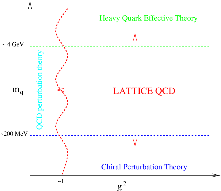
Figure 1: A schematic of the theoretical approaches used to analyze QCD and their domain of reliability in terms of the basic parameters, the strong coupling constant $g$ and quark masses $m_{q}$.

To appreciate the difference between weakly and strongly interacting particles, consider the propagation of an electron and a proton as illustrated in Figs. 2 and 3. The quantum mechanical wavefunction of the electron (called the Fock space wavefunction) is a superposition of the electron propagating undisturbed; the electron propagating by emitting a photon at point $x_{1},t_{1}$ and reabsorbing it at point $x_{2},t_{2}$; emitting two photons at points $x_{1},t_{1}$ and $x_{2},t_{2}$ and reabsorbing them at points $x_{4},t_{4}$ and $x_{3},t_{3}$; emitting a photon at point $x_{1},t_{1}$, the photon generating an electron-positron pair at $x_{2},t_{2}$, which annihilate to produce a photon at $x_{3},t_{3}$, which is reabsorbed by the initial electron at $x_{4},t_{4}$; and so on. These higher order processes are suppressed by the number of times the interaction between the photon and charge takes place. For example, in Fig. 2D, the suppression factor for the amplitude is $g_{em}^{4}$ ($\alpha=g_{em}^{2}/4\pi\approx 1/137$).

Furthermore, these higher order process are “virtual”; $i.e.$ an electron in an eigenstate does not change unless one tries to detect it or there is an interaction with an external source. The very process of detection disturbs the electron and imparts it energy and momentum. Thus, the electron manifests itself as two electrons and a positron a very small fraction of the time unless the probe imparts a lot of energy.

The bottom line is that if the coupling constant associated with a given kind of interaction is small, as is true of electromagnetic and weak interactions, the simplest possibility is dominant and the higher order possibilities are small corrections. These corrections can be calculated analytically as a power series expansion in the coupling. The most striking and successful example of this approach is the calculation of the anomalous magnetic moment of the electron $a_{e}=0.5(g_{e}-2)$. Kinoshita and collaborators [3] calculated 891 4-loop diagrams (Fig. 2C,D are examples of 2-loop diagrams), and find

$$a_{e}(theory) = 0.5\big{(}\alpha/\pi\big{)}+$$ (1)

$$- 0.328\ 478\ 965\ \ldots\big{(}\alpha/\pi\big{)}^{2}$$

$$+ 1.181\ 241\ 456\ \ldots\big{(}\alpha/\pi\big{)}^{3}$$

$$- 1.409\ 2\ (384)\ \ldots\big{(}\alpha/\pi\big{)}^{4}$$

$$+ 4.396\ (42)\ \times 10^{-12},$$

to be compared with the experimental measurements

$$a_{e^{-}}(exp) = 1\ 159\ 652\ 188.4\ (4.3)\ \times 10^{-12}$$

$$a_{e^{+}}(exp) = 1\ 159\ 652\ 187.9\ (4.3)\ \times 10^{-12}\,.$$ (2)

To confront theoretical prediction with experimental numbers one needs an independent measurement of the electromagnetic coupling $\alpha$. It turns out that the uncertainty in the measurements of $\alpha$ from the quantum Hall effect, the ac Josephson effect, and the de Broglie wavelength of the neutron beam, are large enough to deny a resolution of this issue! So in fact the authors have turned the question around $--$ assume QED is correct and use $a_{e}$ to determine $\alpha$! This example should convince you that very precise predictions of QED can be extracted using perturbation theory; the exception being when many-body effects are important as for example in some condensed matter systems. The same is true of weak interactions as these are governed by an even smaller coupling. Parenthetically it is worth highlighting that this “analytical” calculation [3] could not have been done without the resources of a massively parallel computer.

     

Figure 2: A schematic of the virtual processes, (B) to (D), associated with the propagation of a ‘bare’ electron, (A)

Before discussing QCD, it is worth mentioning that the coupling constant in QFT is not a fixed constant. Quantum fluctuations in the form of virtual particles discussed above can screen or anti-screen the charge. As a result, the strength of interactions depends on the energy of the probe. In QCD the coupling is large, $O(1)$, for energy scales $\mathrel{\raise 2.0pt\hbox to8.0pt{\raise-5.0pt\hbox{$\sim$}\hss{$<$}}}1$ GeV (typical of nuclear matter), and becomes weak with increasing energy. This is why perturbative methods are reliable for describing high energy collisions (small $g$ region in Fig. 1), while non-perturbative methods like lattice QCD are essential at nuclear energy scales.

In Fig. 3B I have shown the virtual process in which the intermediate state of a proton is a neutron and a pion. Once again the leading contribution is $g_{s}^{4}$, however since $\alpha_{s}=g_{s}^{2}/4\pi\sim 1$, this and other such “higher” order processes are not suppressed. Thus the situation in the case of strong interactions, described by QCD, is completely different. QCD is a highly non-linear, strongly interacting theory characterized by $\alpha_{s}\sim 1$ for processes involving momentum transfers of $\mathrel{\raise 2.0pt\hbox to8.0pt{\raise-5.0pt\hbox{$\sim$}\hss{$<$}}}1$ GeV. As a result perturbative calculations based on keeping a few low order Feynman diagrams are not reliable. One has to include essentially all exchanges of soft gluons, $i.e.$ devise non-perturbative approaches. Large scale numerical simulations of lattice QCD are currently the most promising possibility; in this approach contributions of all possible interactions via the exchange of gluons with momentum smaller than the lattice cutoff $2\pi/a$ are included.

     

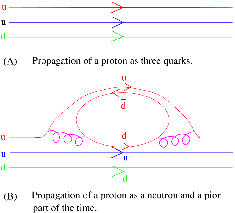
Figure 3: A schematic of the propagation of a proton. Part of the time it is in the intermediate virtual state of a neutron and a pion.

4 QCD

Deep inelastic scattering experiments, scattering of very high energy electrons off protons and neutrons, carried out in the late sixties and early seventies at SLAC showed that the latter were composite. They were bound states of even more fundamental particles which were given the name quarks by Gell-Mann (or aces by Zweig). These quarks carried, in addition to the electromagnetic charge $e/3$ or $2e/3$, a strong charge that was dubbed color. If QFT were to explain the experiments, three generalizations to QED were required. First, the color charge had to occur in three varieties (which were called red, blue, and green) but each with the same strength. Second, the value of this charge had to depend on the energy, it was strong at low energies and progressively got weaker as the energy was increased. Third, the quarks were always confined within hadrons as no experiment had detected an isolated quark. It turned out that a generalization of QED with precisely these additional features had been proposed, in a different context, in 1954 by Yang and Mills [4]. This mathematical theory adapted to the features seen in strong interactions is called QCD.

In QCD, quarks can carry any one of the three colors and anti-quarks carry anti-color. The interactions between them is via the exchange of gluons which themselves carry color. Thus, a red quark can turn into a green quark by the emission of a red-antigreen gluon. Similarly a green quark and an anti-green anti-quark can annihilate into a green anti-green gluon or a photon which has no strong charge. The fact that gluons, unlike photons, also carry the color charge makes QCD a much more non-linear theory than QED.

One way confinement can arise is if the potential energy between a quark and antiquark (or two quarks) grows linearly with distance, consequently it would take an infinite amount of energy to isolate them. The hadrons we detect in experiments would have to be color neutral. There are two types of color neutral objects one can form with this three color theory, mesons made up of a quark and an antiquark with the corresponding anti-color, and baryons with three quarks having different colors but in a color neutral combination. The mathematical structure that encapsulates these ideas is the non-abelian group of $3\times 3$ unitary matrices with unit determinant, SU(3). The quarks are assigned to the fundamental representation 3 of SU(3) and anti-quarks to the $\bf{\bar{3}}$. The color neutral mesons and baryons are the combinations that transform as singlets, $i.e.$ the identity representation in $3\otimes\bar{3}=1\oplus 8$ and $3\otimes 3\otimes 3=1\oplus 8\oplus 8\oplus 10$ respectively. For a more detailed introduction to QFT and QCD see [1].

To explain the plethora of hadrons that had already been seen in experiments by the early sixties, it was postulated that quarks have yet another label (internal quantum number) called flavor. As of today, experiments have revealed six flavors, which are called up, down, strange, charm, beauty, and top, and the strong interactions are observed to be the same for all. This replication in nature of quarks with flavor is very similar to that seen in the case of leptons; electrons, muons, and tau have identical electromagnetic interactions and differ only in their mass. There is, however, one major difference. We need at least two flavors, up and down quarks, to form neutrons and protons. These, along with electrons, are the building blocks of all matter.

All these features of strong interactions are neatly summarized in the Yang-Mills action density

$$S(x)=\sum_{flavors}^{i}\ \sum_{colors}^{a,b}\overline{\psi}^{i,a}(x)\big{[}i\gamma_{\mu}(\partial_{\mu}\delta^{ab}-igG_{\mu}^{a,b})-m_{i}\big{]}\psi^{i,b}$$ (3)

where $G_{\mu}=1/\sqrt{2}\sum_{i}T^{i}A_{\mu}^{i}$ is the matrix of gauge fields and the $T^{i}$ are the eight generators of SU(3). The action for the gauge fields is

$$S_{gauge}(x) = -1/2{\rm Tr}F^{\mu\nu}F_{\mu\nu}$$

$$F_{\mu\nu}^{a} = \partial_{\mu}G_{\nu}^{a}-\partial_{\nu}G_{\mu}^{a}+gf^{abc}G^{b}_{\mu}G^{b}_{\nu}\,.$$ (4)

This action has an exact invariance under local (independent at each and every space-time point) transformations in the color variables, again a generalization of the gauge transformation of QED. The only differences from the Dirac action for QED are (i) the color indices in Eqs. 3 and 4, and (ii) the non-linear term in Eq. 4 which arises because the gluons themselves carry charge and are self-interacting. Thus, for small $g$ one can imagine that this non-linear term will be small and a perturbative expansion in $g$ is reliable. This is exactly what happens at very high momentum transfers. On the other hand, when $g$ is large the non-linear effects cannot be neglected and one needs different non-perturbative methods. The method we will discuss is numerical simulations of QCD discretized on a space-time lattice.

5 Overview of the Lattice Approach

LQCD calculations are a non-perturbative implementation of field theory using the Feynman path integral approach. The calculations proceed exactly as if the field theory was being solved analytically had we the ability to do the calculations. The starting point is the partition function in Euclidean space-time

$$Z\ =\ \int\big{[}\prod_{x}{\mathcal{D}}A_{\mu}(x)\ {\mathcal{D}}\psi(x)\ {\mathcal{D}}\bar{\psi}(x)\big{]}\ e^{-S}$$ (5)

where $S$ is the QCD action

$${\mathcal{S}}\ =\ \int d^{4}x\ \big{(}\frac{1}{4}F_{\mu\nu}F^{\mu\nu}(x)-\bar{\psi}M\psi\big{)}\ .$$ (6)

Here $F_{\mu\nu}F^{\mu\nu}(x)$ is the gluon action density and and $M$ is the Dirac operator. The fermions are represented by Grassmann variables $\psi$ and $\bar{\psi}$. Since the action is linear in $\psi$ and $\bar{\psi}$, these can be integrated out exactly using rules of Grassman integration with the result

$$Z\ = \ \int\big{[}\prod_{x}{\mathcal{D}}A_{\mu}(x)\big{]}\ {\rm det}M\ e^{\int d^{4}y\ (-\frac{1}{4}F_{\mu\nu}F^{\mu\nu})}$$ (7)

$$= \ \int\big{[}\prod_{x}{\mathcal{D}}A_{\mu}(x)\big{]}\ e^{\int d^{4}y\ (-\frac{1}{4}F_{\mu\nu}F^{\mu\nu}+\sum_{i}{\log}({\rm Det}M_{i}))}.$$

The second term defines an effective action for the gauge fields

$$S_{eff}\ ={S_{gauge}+S_{quarks}}=\ \int d^{4}x\ \big{(}{1/4}F_{\mu\nu}F^{\mu\nu}\big{)}-\sum_{i}{\log}({\rm Det}M_{i})\,.$$ (8)

The fermionic contribution is now contained in the highly non-local term ${\rm det}M$ which is only a function of the gauge fields. The sum is over the quark flavors, distinguished by the value of the bare quark mass. A key feature of QCD is that the action $S$ is real and bounded from below. Thus Eq. 7 defines a partition function in exact analogy to statistical mechanics systems where $Z=\sum_{configurations}e^{-E/kT}$. The only difference is that instead of the Boltzmann factor $e^{-E/kT}$ we have $e^{-S}$, $i.e.$ the action measured in units of the Planck constant $\hbar$ which is set to unity by an appropriate choice of units. In numerical simulations, this factor is used to define the probability with which to generate the background gauge configurations.

Having generated an ensemble of gauge configurations, results for physical observables are obtained by calculating expectation values

$$\langle{\mathcal{O}}\rangle\ =\ \frac{1}{Z}\ \int\big{[}\prod_{x}{\mathcal{D}}A_{\mu}(x)\big{]}\ {\mathcal{O}}\ e^{-S}\ .$$ (9)

where ${\mathcal{O}}$ is any given combination of operators expressed in terms of time-ordered products of gauge and quark fields. This calculation involves a double infinity due to the continuous valued nature of space-time and the gauge fields $--$ the number of points $x$ are infinite, and at each point $x$ the field $A_{\mu}$ takes on a continuous infinity of values. To make the system finite Wilson [5] made two approximations: (i) he replaced continuous space time by a discrete lattice of finite extent $L$ and spacing $a$, and (ii) he devised a method that generated a representative set of important configurations that allow for a very good approximation to the integral over $A_{\mu}$. The latter is achieved using Monte Carlo methods of integration. On this lattice, the gauge fields $A_{\mu}(x)$ are defined in terms of $3\times 3$ complex matrices $U_{\mu}(x)=\exp(iagA_{\mu}(x))$ and associated with the links between sites $x$ and $x+\hat{\mu}$. The quarks fields in $\mathcal{O}$ are, in practice, re-expressed in terms of quark propagators using Wick’s theorem for contracting fields. In this way all dependence on quarks as dynamical fields is removed. For more details on the discretization of QCD on the lattice see [6, 7].

The basic building block for fermionic quantities is the Feynman propagator,

$$S_{F}(y,j,b;x,i,a)\ =\ \big{(}M^{-1}\big{)}^{y,j,b}_{x,i,a}\,,$$ (10)

where $M^{-1}$ is the inverse of the Dirac operator calculated on a given background field. A given element of this matrix $\big{(}M^{-1}\big{)}^{y,j,b}_{x,i,a}$ is the amplitude for the propagation of a quark from site $x$ with spin-color $i,a$ to site-spin-color $y,j,b$. The matrix $M$ is very large, $12L^{4}\times 12L^{4}$, but very sparse. A given site is connected to only itself and a few neighbors, $i.e.$ a total of 9 points in the case of nearest-neighbor interactions. Thus, in numerical calculations $M$ is not stored but constructed on the fly from the gauge links $U_{\mu}$, which define it completely. The calculation of the inverse is done by solving the set of linear equations

$$M\chi=\phi$$ (11)

where $\phi$ is a source vector (usually taken to be a delta function at one site). The solution $\chi$ is found using a variety of iterative algorithms (Krylov solvers) like conjugate gradient, minimal residue, $etc.$, that include preconditioning and acceleration techniques as discussed by Th. Lippert [8]. In practice we do not construct the entire inverse but only solve for a few columns of $M^{-1}$, $i.e.$ solve Eq. 11 for a few $\phi$, as each column gives the Feynman propagator from a given site to all other sites. Since the theory is invariant under translations, the particular choice of the site does not matter after the sum over configurations.

To summarize, in the Feynman path approach to QFT one needs the ability to (a) generate all possible configurations of gauge fields and (b) calculate a variety of correlation functions on each of these configurations. Expectation values are averages of these correlation functions weighted by the “Boltzmann” factor $e^{-S}$ of each configuration. In the next section I will show how physical observables are extracted from these expectation values.

There is a technical issue, the “quenched” approximation (QQCD), worth highlighting here as it has played a central role in simulations. It consists of setting ${\rm Det}M=constant$ in Eq. 7 [9]. This approximation corresponds to removing the momentum dependence of vacuum polarization effects from the QCD vacuum as illustrated in Fig. 4. The lattice QCD community has resorted to using this approximation out of necessity, full QCD computations are $10^{3}-10^{5}$ times more costly. The quenched results are, nevertheless, useful phenomenologically as this approximation is expected to be good to within $10-20\%$ for many quantities. Also, by doing quenched calculations we understood all other sources of errors, discussed in Section 7, that are similar in both the quenched and full theories and how to control them.

     

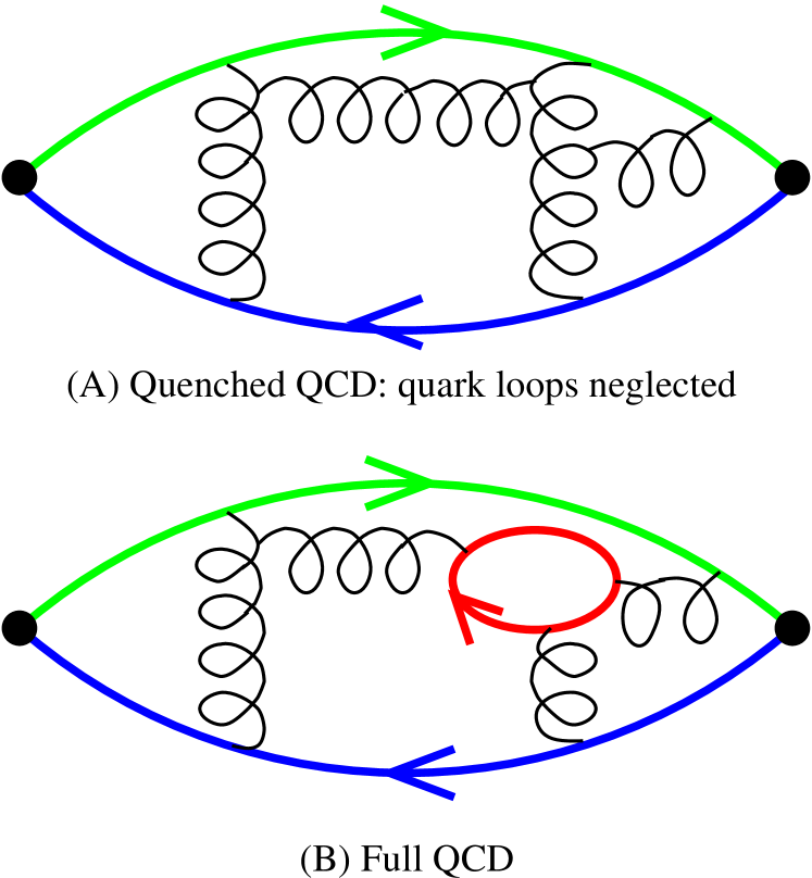
Figure 4: A set of diagrams illustrating the quenched approximation. In it all possible gluon exchanges are allowed but without the possibility of internal quark loops (vacuum polarization).

6 Physics from Numerical Simulations

In the last section I outlined the calculation of expectation values. Here I will illustrate how to extract physical observables from these using as an example the mass $M_{\pi}$ and the decay constant $f_{\pi}$ of the pion.

Consider the 2-point correlation function, $\langle 0|T[\sum_{x}{\mathcal{O}}_{f}(\vec{x},t){\mathcal{O}}_{i}(\vec{0},0)]|0\rangle$ with $t>0$, where the operators ${\mathcal{O}}$ are chosen to be the fourth component of the axial vector current ${\mathcal{O}}_{f}={\mathcal{O}}_{i}=A_{4}=\bar{\psi}\gamma_{4}\gamma_{5}\psi$ as these have a large coupling to the pion. This 2-point correlation function gives the amplitude for creating a state with the quantum numbers of the pion out of the vacuum at space-time point $0$ by the “source” operator ${\mathcal{O}}_{i}$; the evolution of this state to the point $(\vec{x},t)$ via the QCD Hamiltonian; and finally the annihilation by the “sink” operator ${\mathcal{O}}_{f}$ at $(\vec{x},t)$. The rules of quantum mechanics tell us that ${\mathcal{O}}_{i}$ will create a state that is a linear combination of all possible eigenstates of the Hamiltonian that have the same quantum numbers as the pion, $i.e.$ the pion, radial excitations of the pion, three pions in $J=0$ state, $\ldots$. The second rule is that after propagating for Euclidean time $t$, a given eigenstate with energy $E$ picks up a weight $e^{-Et}$. Thus, the 2-point function can be written in terms of a sum over all possible intermediate states

$$\langle 0|\sum_{x}{\mathcal{O}}_{f}(\vec{x},t){\mathcal{O}}_{i}(0)|0\rangle=\sum_{n}\frac{\langle 0|{\mathcal{O}}_{f}|n\rangle\langle n|{\mathcal{O}}_{i}|0\rangle}{2E_{n}}\ e^{-E_{n}t}\,.$$ (12)

To study the properties of the pion at rest we need to isolate this state from the sum over $n$. To do this, the first simplification is to use the Fourier projection $\sum_{\vec{x}}$ as it restricts the sum over states to just zero-momentum states, so $E_{n}\to M_{n}$. (Note that, by momentum conservation it is sufficient to make the Fourier projection over either ${\mathcal{O}}_{i}$ or ${\mathcal{O}}_{f}$.) The second step to isolate the pion, $i.e.$ project in the energy of the state, consists of a combination of two strategies. One, make a clever choice of the operators ${\mathcal{O}}$ to limit the sum over states to a single state (the ideal choice is to set ${\mathcal{O}}$ equal to the quantum mechanical wave-functional of the pion), and two, examine the large $t$ behavior of the 2-point function where only the contribution of the lowest energy state that couples to ${\mathcal{O}}_{i}$ is significant due to the exponential damping. Then

$$\langle 0|\sum_{x}{\mathcal{O}}_{f}(x,t){\mathcal{O}}_{i}(0)|0\rangle\ \ \mathrel{\raise 2.0pt\hbox to24.0pt{\raise-8.0pt\hbox{$t\to\infty$}\hss{$=$}}}\ \ \ \ \frac{\langle 0|{\mathcal{O}}_{f}|\pi\rangle\langle\pi|{\mathcal{O}}_{i}|0\rangle}{2M_{\pi}}\ e^{-M_{\pi}t}\,.$$ (13)

The right hand side is now a function of the two quantities we want since $\langle 0|A_{4}(\vec{p}=0)|\pi\rangle=M_{\pi}f_{\pi}$. In this way, the mass and the decay constant are extracted from the rate of exponential fall-off in time and from the amplitude.

Let me now illustrate how the left hand side of Eq. 13 is expressed in terms of the two basic quantities we control in the path integral – the gauge fields and the quark propagator. Using Wick contractions [1], the correlation function can be written in terms of a product of two quark propagators $S_{F}$,

$$-\langle 0|\sum_{x}\bar{\psi}(x,t)\gamma_{4}\gamma_{5}\psi(x,t) \bar{\psi}(0,0)\gamma_{4}\gamma_{5}\psi(0,0)|0\rangle$$ (14)

$$\hskip-43.36243pt\equiv\langle 0|\sum_{x}S_{F}(0;\vec{x},t)\gamma_{4}\gamma_{5}S_{F}(\vec{x},t;0)\gamma_{4}\gamma_{5}|0\rangle\,.$$

and the $\gamma_{i}$ which are the Dirac spin matrices. This is the expectation value we measure as a function of $t$. By equating its large $t$ behavior to the expected form, Eq.(13), we can extract the mass $M_{\pi}$. The decay constant $f_{\pi}$ is obtained from the amplitude using the relation $\langle 0|A_{4}|\pi\rangle=M_{\pi}f_{\pi}$.

Once we have the ability to isolate a given state from the large $t$ behavior there are a number of matrix elements we can calculate from 2-point, 3-point, $\ldots$, correlation functions. Examples are

• $\langle 0|A_{4}(\vec{p}=0)|\mathcal{P}\rangle$. This gives the decay constant for a pseudoscalar hadron $\mathcal{P}$ which can be a $\pi$, K, D, or B meson.

• $\langle{\mathcal{H}}(\vec{p},\vec{s})|{\mathcal{O}}_{T}^{n}|{\mathcal{H}}(\vec{p},\vec{s})\rangle$. These matrix elements give the $n^{th}$ moment of the momentum distribution of quarks and gluons inside the hadron ${\mathcal{H}}$. Here $T$ labels the “twist” of the operator. These distributions are measured in deep-inelastic scattering experiments.

• $\langle{\mathcal{H}}(\vec{p})|{\mathcal{J}}_{\mu}(\vec{p})|{\mathcal{H}}(\vec{p}=0)\rangle$, where ${\mathcal{J}}_{\mu}$ is the electromagnetic current. These matrix elements probe the charge and current distributions within a hadron ${\mathcal{H}}$ by measuring the electromagnetic form-factors.

• $\langle\pi(\vec{p})|{\mathcal{V}}_{\mu}(\vec{p})|{\mathcal{B}}(\vec{p}=0)\rangle$ and $\langle\pi(\vec{p})|{\mathcal{A}}_{\mu}(\vec{p})|{\mathcal{B}}(\vec{p}=0)\rangle$ probe the form-factors that parameterize the semileptonic decays like $B\to\pi\mu\nu_{\mu}$. These are used to extract the Cabibbo-Kobayashi-Maskawa matrix elements that describe the mixing between quarks of different flavors under weak interactions.

• $\langle K^{0}|\bar{s}_{L}\gamma_{\mu}d\bar{s}_{L}\gamma_{\mu}d|\overline{K^{0}}\rangle$ and $\langle B^{0}|\bar{b}_{L}\gamma_{\mu}d\bar{b}_{L}\gamma_{\mu}d|\overline{B^{0}}\rangle$ are the amplitudes for the $K^{0}\leftrightarrow\overline{K^{0}}$ and $B^{0}\leftrightarrow\overline{B^{0}}$ mixing. These play an improtant role in the extraction of the CP violation parameters $\epsilon_{K},\epsilon_{B}$ and consequently of the Wolfenstein parameters $\rho$ and $\eta$ [10].

• $\langle\pi\pi|{\mathcal{H}}_{W}|\overline{K^{0}}\rangle$. These are the matrix elements of the effective weak Hamiltonian describing the weak decays $K\to\pi\pi$. These matrix are needed to understand the $\Delta I=1/2$ rule and in the calculation of the CP violating parameter $\epsilon^{\prime}/\epsilon$ [10]. .

Many simulations testing the efficacy of lattice techniques for calculating these matrix elements, spectrum of mesons, baryons, glueballs, the behavior of QCD at finite temperature, and the nature of the QCD vacuum have been carried out since the pioneering work by Creutz [11] and Wilson [12] in the late seventies. The current status of these calculations is reported in the proceedings of the annual conferences on Field Theory on the Lattice [13].

7 Computational challenges posed by LQCD

It is self-evident that given a very precise theory (QCD) and a well defined method to solve it numerically (Monte Carlo integration of lattice QCD), the success of the calculations depends on the size of the statistical and systematic errors compared to the desired precision. A brief outline of the systematic errors is as follows.

• Finite lattice spacing errors: To make the Feynman path integral finite, a discrete space-time grid with spacing $a$ is introduced. The continuum theory is recovered in the limit $a\to 0$. This limit is taken by extrapolation. At finite $a$ there are discretization errors; for example $(f(x+a)-f(x))/a=\partial_{x}f(x)+a/2\partial_{x}^{2}f(x)+\ldots$ implies that using such a finite difference to approximate a derivative will lead to errors proportional to $a$. These errors, as explained by P. Lepage [14], are being understood and reduced by using (a) a generalization of higher order difference schemes that takes quantum effects into account and (b) doing the calculations at a number of values of $a$ in the range $2<1/a<5$ GeV and then extrapolating to $a=0$.

• Finite Volume errors: A finite periodic box distorts the spectrum of particles. However, it has been determined empirically that for $M_{pion}L>5$ these corrections are exponentially suppressed and less than $1\%$. The lattice sizes needed to ensure this condition are, for the quenched theory, accessible on computers with 100 Gigaflops sustained performance (see the article by A. Ukawa[22]).

• Quenched Approximation: The quenched approximation distorts the vacuum state of QCD by changing the statistical weight of the background gauge configurations. Intuition and model calculations suggest that this approximation is valid at the $10-20\%$ level for many quantities. In principle, there exist algorithms to simulate QCD without making this approximation as discussed by A. Kennedy, Ph. de Forcrand and Th. Lippert [15, 16, 8]. However, doing so increases the computational time by a factor of $10^{3}-10^{5}$ depending on the value of the quark mass. I believe that calculations done in the next five years using current improved algorithms will be able to completely remove this approximation provided we can have access to computers with $10-100$ Teraflop sustained performance.

• Chiral Extrapolation: The physical up and down quarks are very light ($2-8$ MeV). Iterative algorithms used to solve for quark propagators (obtained by inverting the Dirac matrix) exhibit critical slowing down that goes as $1/m_{quark}$ [8]. As $m_{quark}\to 0$, the cost for quenched calculations goes up as $L^{6}$ and for unquenched as $L^{8-9}$, where $L$, for fixed $a$, has to be increased such that $M_{pion}L\propto\sqrt{m_{quark}}L$ stays constant. There is good theoretical basis to expect that it will be sufficient to calculate physical quantities involving these light quarks over the range $m_{s}-m_{s}/8$ and then extrapolate to $m_{u},\ m_{d}\sim m_{s}/25$ using relations derived from chiral perturbation theory. Since current quenched calculations go down to $m_{s}/4$ and unquenched to only $m_{s}$, current data for some quantities has significant uncertainty due to the chiral extrapolation.

• Discretization of Heavy Quarks: Heavy quarks, in particular the bottom quark with mass $m_{b}\sim 5$ GeV, has a different problem. It’s Compton wavelength is too small compared to $a$ for $2<1/a<5$ GeV. Thus the associated discretization errors are large. Fortunately, novel approaches like the Heavy Quark Effective Theory [17] and Non-relativistic QCD [18] have shown great promise for studying the physics of $b$ quarks.

• Relation between continuum and lattice quantities: One of the subtleties of QFT is figuring out the correct normalization of operators used to calculate matrix elements. These normalization constants are essential to relate lattice results to those measured in experiments. In the last five years, the technology to calculate these constants as part of the non-perturbative lattice calculations has also been developed and tested [19]. The associated uncertainty has, therefore, been significantly reduced.

As of 1999, the two major remaining systematic uncertainties are the quenched approximation and the discretization of bottom quarks. A number of very precise quenched calculations have been done as discussed in the articles of F. Rapuano [21] and S. Aoki et al. [24] in this volume. The new generation of calculations including the effects of dynamical quarks will steadily tune the sea quark masses towards the physical values of $m_{u}$, $m_{d}$, and $m_{s}$. By comparing these results against the precise quenched estimates, we shall be able to systematically quantify the effects of vacuum polarization and finally get phenomenologically useful numbers with all sources of errors estimated.

8 Why Parallel Computers

From a computational point, numerical algorithms used to simulate lattice QCD have certain simplifying features. The calculations are homogeneous and the interactions are local. The first feature implies that exactly the same operations need to be done at each space-time point. It is therefore trivial to maintain synchronization between points. The second feature implies that only a few neighboring points are connected at best. Thus data dependence is only between small blocks, say $2^{4}-4^{4}$, or none at all in the most time consuming part of the calculation (inversion of the Dirac operator to get the quark propagator). One can therefore process a point in each of these blocks simultaneously. In short, the problem is tailor made for distributed/parallel computing (see articles by S. Güsken and Th. Lippert  [23, 8]).

The 4-dimensional space-time grid is divided into smaller hypercubes, and the data and calculations needed to process all the sites within these smaller hypercubes is allocated to each processor. For example a $64^{4}$ lattice can be distributed as $16^{4}$ sub-lattices on 256 processors set up as a $4^{4}$ computational grid to maintain the spatial proximity of the data. Points internal to this $16^{4}$ volume need no information from neighboring processors and get the maximum throughput allowed by the single processor’s speed. Points on the boundary need communications. These communications are again homogeneous. For example each processor needs information from the processor on the right and simultaneously needs to send information to the processor on the left. Furthermore, one almost always uses periodic boundary conditions which makes this pattern of communications cyclic on the 4-dimensional grid of processors. Lastly, one can overlap computations and communications. The communications of boundary points can be initiated while the points internal to the $16^{4}$ volume are being processed. The only constraint is the amount of per processor memory to store this extra data. This, on todays computers, is not a major hurdle.

The Achilles heel of large distributed computers is inter-node communication speed and memory bandwidth if commodity processors are to be used. In this regard too LQCD calculations are ideally suited for implementation on parallel computers (see the articles of S. Aoki et al., R. Mawhinney, and R. Tripiccione in this volume [24, 25, 26].) One can examine the worst case senerio of the penalty imposed by communications in case overlap of communication and computation is not allowed by either the hardware or the software. The basic arithmetic unit in LQCD calculations is the multiplication of a complex $3\times 3$ matrix with a $3\times 1$ complex vector, where the latter may need communication to a neighboring node. Thus, one performs $66$ flops for every $24$ bytes communicated. In practice the situation is even better as data for only the points on the boundary of the hypercube in each node need communication. Lastly, global sums and/or global broadcasts, which are potentially slow, are not done often enough to be a significant overhead.

Accepting the fact that simulations of LQCD are tailor made for parallel computing, it should come as no surprise that theoretical physicists interested in solving QCD have been in the thick of the development of parallel computers. The “cosmic cube” at Caltech (1982), the Columbia University special purpose machines (since 1982), the APE computers of INFN at Rome and Pisa (since 1986), the GF11 supercomputer at IBM (1986-1997), and the Japanese projects at Tsukuba University (QCDPAX and CP-PACS) are examples of such projects that have successfully produced Lattice QCD results. In addition, the lattice QCD community has also been amongst the first and most efficient users of commercial supercomputers of all kinds: vector(CRAYS, ETA10) and/or parallel (Connection Machines, Intel hypercube and Paragon, IBM SP2, Silicon Graphics Origin 2000). Consequently, they have contributed to the overall development of high performance computing by educating a generation of skilled computational scientists, interacting with computer vendors to help optimize and test new hardware and software, and providing an environment and an example that motivated other communities to use emergent architectures.

9 Outlook

Progress in understanding QCD (mechanisms for confinement and chiral symmetry breaking), verifying QCD (reproducing the hadron spectrum), calculating strong corrections to weak matrix elements, and elucidating the behavior of QCD at finite temperature has required a combination of four things. (i) Better theoretical understanding and formulation of quantities to calculate: (ii) Better ways of discretizing QCD as discussed in [14, 27]: (iii) More efficient numerical algorithms for the generation of background configurations and quark propagators [8]: And (iv) higher performance specifically designed computers and their exploitation [21, 24, 25, 26]. The field has witnessed significant developments in all four areas during the last twenty years. In computing power we have evolved from VAXes ($\sim 1$ Megaflop with 4 Megabytes of RAM) to CP-PACS (600 Gigaflops and 128 Gigabytes of RAM). As a result we have been able to simulate bigger lattices and do more precise calculations. These in turn have motivated the development of new algorithms and techniques as discussed in succeeding articles.

I would like to characterize the first twenty years (1979-1998) of lattice QCD as the taming of the quenched approximation. We have now calculated many quantities with sufficient precision that the largest remaining uncertainty is the quenched approximation. Future calculations will steadily chip away at this last uncontrolled source of systematic error. In five years time (year 2004), I anticipate we shall have access to machines of 10 Teraflops sustained performance, and will have developed and tested various theoretical and numerical enhancements that will allow us to obtain the same quality of results for the full theory. So, it is an exciting coincidence that as we enter the new millenia, we have a new powerful tool, the computer, that will allow us to reliably calculate the properties of QCD, a fundamental theory of nature, from first principles.

Acknowledgements

It is a pleasure to thank Nicola Cabibbo, Yoichi Iwasaki, and Klaus Schilling for inviting me to contribute to this special issue.

References

- [1] C. Quigg, Gauge Theories of Strong, Weak, and Electromagnetic Interactions, Benjamin/Cummings, 1983; F. Halzen and A. D. Martin, An Introductory Course in Modern Particle Physics, Wiley, 1984. M. E. Peskin and D. V. Schroeder, An Introduction to Quantum Field Theory, Addisen-Wesley, 1995.
- [2] A. Pich, Lectures at the 1997 Les Houches Summer School “Probing the Standard Model of Particle Interactions”, Eds. R. Gupta, A. Morel, E. de Rafael, and F. David, North Holland, 1999.
- [3] T. Kinoshita, in Recent Advances in Hadron Physics, Eds. K. Kang, S. Kim, C. Lee, World Scientific, 1998.
- [4] C. N. Yang, and R. L. Mills, .
- [5] K. Wilson, .
- [6] M. Creutz, Quarks, Gluons, and Lattices, Cambridge University Press, 1983.
- [7] R. Gupta, in Proceedings of 1997 Les Houches Summer School ibid.
- [8] Th. Lippert, this volume.
- [9] H. Hamber and G. Parisi, ; E. Marinari, G. Parisi, and C. Rebbi, ; D. Weingarten,
- [10] A. Buras, in the proceedings of the 1997 Les Houches school, ibid.
- [11] M. Creutz,
- [12] K. Wilson, in Recent Developments in Gauge Theories, edited by G. t’Hooft, et al., Plenum Press, N.Y. 1980.
- [13] LATTICE93 ; LATTICE94 ; LATTICE95 ; LATTICE96 ; LATTICE97 .
- [14] G. P. Lepage, this volume.
- [15] A. Kennedy, this volume.
- [16] Ph. de Forcrand, this volume.
- [17] E. Eichten and B. Hill, , ; .
- [18] P. Lepage and B. Thacker, ; G. Lepage, L. Magnea, C. Nakhleh, U. Magnea and K. Hornbostel, .
- [19] T. Bhattacharya, S. Chandrasekhar, R. Gupta, W. Lee, and S. Sharpe, hep-lat9810018.
- [20] N. Christ, this volume.
- [21] F. Rapuano, this volume.
- [22] A. Ukawa, this volume.
- [23] S. Güsken, this volume.
- [24] S. Aoki et al, this volume.
- [25] R. Mawhinney, this volume.
- [26] R. Tripiccione, this volume.
- [27] R. Edwards, U. Heller, and R. Narayanan, this volume.