CERN-TH/99-124

hep-lat/9905004

THE NON-PERTURBATIVE QCD DEBYE MASS
FROM A WILSON LINE OPERATOR

M. Laine^a,b,, O. Philipsen^a,

^aTheory Division, CERN, CH-1211 Geneva 23, Switzerland
^bDept. of Physics, P.O.Box 9, FIN-00014 Univ. of Helsinki, Finland

Abstract

According to a proposal by Arnold and Yaffe, the non-perturbative $g^{2}T$-contribution to the Debye mass in the deconfined QCD plasma phase can be determined from a single Wilson line operator in the three-dimensional pure SU(3) gauge theory. We extend a previous SU(2) measurement of this quantity to the physical SU(3) case. We find a numerical coefficient which is more accurate and smaller than that obtained previously with another method, but still very large compared with the naive expectation: the correction is larger than the leading term up to $T\sim 10^{7}T_{c}$, corresponding to $g^{2}\sim 0.4$. At moderate temperatures $T\sim 2T_{c}$, a consistent picture emerges where the Debye mass is $m_{D}\sim 6T$, the lightest gauge invariant screening mass in the system is $\sim 3T$, and the purely magnetic operators couple dominantly to a scale $\sim 6T$. Electric ($\sim gT$) and magnetic ($\sim g^{2}T$) scales are therefore strongly overlapping close to the phase transition, and the colour-electric fields play an essential role in the dynamics.

CERN-TH/99-124
May 1999

1 Introduction

An important concept in the description of the deconfined finite temperature QCD plasma is the Debye mass $m_{D}$. It is the inverse of the spatial screening length felt by colour-electric excitations, in analogy with Debye screening in abelian plasmas, which is felt by electric fields but not by magnetic fields. The leading order result for $m_{D}$ is perturbatively computable [1], but the next-to-leading order result is already non-perturbative [2], making the determination of $m_{D}$ (and, in fact, already its precise definition) a challenging theoretical problem. The numerical value of $m_{D}$ has a number of applications, in particular in the phenomenology for quark-gluon plasma formation (for a review, see [3]). It is also interesting to note that, even though $m_{D}$ is originally a strictly static quantity, it might have significance even for some dynamical observables, such as the rates of anomalous processes in the plasma [4].

A gauge invariant, non-perturbative definition for $m_{D}$ has been given by Arnold and Yaffe [5]. This definition is based on a (Euclidian) time reflection operation, denoted also by ${\cal R}_{z}$, which reverses the sign of the temporal component of the gauge field: ${\cal R}_{z}A_{0}^{a}\to-A_{0}^{a}$ (for a more detailed discussion, see [5]). The Debye mass is defined as the smallest among the exponential fall-offs that are found for gauge invariant operators odd under this symmetry. A further observation is that due to finite temperature dimensional reduction [6]–[9], the measurement of $m_{D}$ in numerical simulations can be carried out in a three-dimensional (3d) SU(N) + adjoint Higgs theory. Lattice measurements in this theory were performed, both for SU(2) and SU(3), in [10].

However, there is a problem in making precise simulations in the 3d SU(3) + adjoint Higgs theory. The reason is that in the regime of asymptotically small couplings, there is a scale hierarchy between the leading order result $m_{D}\sim gT$ and the non-perturbative correction $\delta m_{D}\sim g^{2}T$, which one is trying to determine (the “magnetic” degrees of freedom are also associated with the scale $g^{2}T$). As always, a scale hierarchy is difficult to accommodate on a single lattice of presently available sizes, and thus makes the approach to the continuum limit quite problematic in practical simulations.

Fortunately, there is a way out: parametrically (i.e., as a power series in $g$), even the field $A_{0}^{a}$ can be integrated out perturbatively, leaving a pure 3d SU(3) gauge theory. The operator odd in $A_{0}^{a}$ goes over to a non-local but gauge invariant Wilson line in the pure SU(3) gauge theory [5]. This allows to determine the coefficient of $g^{2}T$.

For the SU(2) case, this Wilson line operator was studied with lattice simulations in [14]. We found a result for the $g^{2}T$ term which is more precise and smaller than that found in [10]. The purpose of the present paper is to extend the SU(2) measurement to the physical SU(3) case.

2 The operator in the continuum

Let us start by briefly reviewing the basic idea of the approach in [5]. Consider gauge invariant operators $O(x)$ odd under $A_{0}\to-A_{0}$ (i.e., in the notation of [5], with ${\cal R}_{z}=-1$). In practice, we consider $O(x)$ containing only one power of $A_{0}$, since otherwise (for $A_{0}^{n},n\geq 3$) the leading behaviour for small $g$ is expected to be of the form $n\cdot m_{0}$, where $m_{0}=(N/3+N_{f}/6)^{1/2}gT$ is the leading order Debye mass [1] ($N_{f}$ is the number of flavours). Imagine now doing the path integral over $A_{0}$ before doing that over $A_{i}$. Then,

$$\frac{\int\!{\cal D}A_{0}\,O(x)O(y)\exp(-S_{A_{0}})}{\int\!{\cal D}A_{0}\,\exp(-S_{A_{0}})}\sim O^{\prime}_{a}(x)G^{ab}(x,y)O^{\prime}_{b}(y),$$ (1)

where $O^{\prime}=dO/dA_{0}$,

$$S_{A_{0}}=\int\!d^{3}x\,\Bigl{[}{\frac{1}{2}}(D_{i}A_{0})^{a}(D_{i}A_{0})^{a}+{\frac{1}{2}}m_{0}^{2}A_{0}^{a}A_{0}^{a}\Bigr{]},$$ (2)

and $G^{ab}(x,y)$ is the tree-level Green’s function in the background of $A_{i}$:

$$G^{ab}(x,y)=\frac{\exp(-m_{0}|x-y|)}{4\pi|x-y|}W^{ab}(x,y),$$ (3)

with $W^{ab}(x,y)$ the adjoint Wilson line,

$$W^{ab}(x,y)=2{\rm Tr\,}T^{a}W^{\rm fund}(x,y)T^{b}[W^{\rm fund}(x,y)]^{\dagger},$$ (4)

where $W^{\rm fund}(x,y)={\cal P}\exp({ig\int_{x}^{y}\!dx_{i}A_{i}^{a}T^{a}})$.

Thus, the measurement of the Debye mass can be reduced to the measurement of

$$G_{F}(x,y) \equiv \left\langle O_{a}^{\prime}(x)W^{ab}(x,y)O_{b}^{\prime}(y)\right\rangle,$$ (5)

in the pure SU(N) gauge theory. The measurement of this operator produces an exponential decay with a coefficient $m$, to which the perturbative part $m_{0}$ from Eq. (3) has to be added in order to obtain the physical result.

Including also loop corrections (i.e., allowing $A_{i}$ to fluctuate at all length scales), maintains the form of the answer but replaces the perturbative $m_{0}$ in Eq. (3) by an effective parameter $m_{0}^{\mbox{\scriptsize eff}}$ [5]:

$$m_{0}\to m_{0}^{\mbox{\scriptsize eff}}=m_{0}+\frac{Ng_{3}^{2}}{4\pi}\biggl{(}\ln\frac{m_{0}}{\Lambda}+d_{\Lambda}\biggr{)}+{\cal O}\biggl{(}g_{3}^{2}\frac{m_{0}}{\Lambda},\frac{g_{3}^{4}}{m_{0}},...\biggr{)},$$ (6)

where $g_{3}^{2}=g^{2}T$, $\Lambda$ is some ultraviolet cutoff, and $d_{\Lambda}$ depends on $\Lambda$. In particular, in the case of a lattice regularization, $\Lambda=a^{-1}$ and $d_{\Lambda}=-(3\ln 2+1)/2$ (see [5, 14]). It follows that if the physical Debye mass is written as

$$m_{D}=m_{0}+{Ng_{3}^{2}\over 4\pi}\ln{m_{0}\over g_{3}^{2}}+c_{N}g_{3}^{2}+{\cal O}(g^{3}T),$$ (7)

then

$$c_{N}=\frac{m}{g_{3}^{2}}+\frac{N}{8\pi}\left(\ln\frac{N^{2}}{2\beta_{G}^{2}}-1\right),$$ (8)

where $m$ is the mass measured from the operator in Eq. (5), and $\beta_{G}=2N/(ag_{3}^{2})$.

We thus need to find operators $O^{\prime}$ such that we get the lowest possible coefficient for the exponential falloff in Eq. (5). From [10], we expect the operators for Eq. (1) to be $O\sim\epsilon_{3jk}{\rm Tr\,}A_{0}F_{jk}$ and suitable variants thereof (see below), leading to $O^{\prime}_{a}=F^{a}_{jk}$ in Eq. (5). In principle, one could get rid of the specification of the operators altogether by measuring the coefficient of the perimeter law of the adjoint Wilson loop [5]. However, in practice the perimeter law can only be observed on the lattice by including this very kind of operators in the basis, due to a very small overlap of the lattice Wilson loop with the asymptotic lightest state [15].

3 A lattice formulation

On the lattice, we replace Eq. (5) with operators of the type

$$G_{F,ijkl}(x,y)=\left\langle 4{\rm Tr\,}(F_{ij}(x)T^{a})\Gamma^{ab}(x,y){\rm Tr\,}(F_{kl}(y)T^{b})\right\rangle,$$ (9)

where $F_{ij}$ is the naive lattice analogue of the field strength tensor,

$$F_{ij}(x)=-\frac{i}{2}\Bigl{[}P_{ij}(x)-P^{\dagger}_{ij}(x)\Bigr{]},$$ (10)

$P_{ij}$ is the plaquette, and $\Gamma^{ab}$ is the lattice Wilson line:

$$\Gamma^{ab}(x,y) = 2{\rm Tr\,}\left(T^{a}S(x,y)T^{b}S^{{\dagger}}(x,y)\right),$$ (11)

$$S(x,y) = \prod_{n=0}^{N-1}U_{3}(x+n\hat{3}),\qquad y=x+N\cdot\hat{3}.$$ (12)

Here $U_{i}$ is a link variable and $\hat{3}$ is the unit vector in the $x_{3}$-direction. Eq. (9) may be rewritten as

$$G_{F,ijkl}(x,y) = 2\left\langle{\rm Tr\,}\left[F_{ij}(x)SF_{kl}(y)S^{{\dagger}}\right]-\frac{1}{N}{\rm Tr\,}F_{ij}(x){\rm Tr\,}F_{kl}(y)\right\rangle,$$ (13)

where the latter term vanishes fast close to the continuum limit and is not numerically important (for SU(2), it vanishes identically). In our simulations, we use $G_{F}$ in this last form, with the components $ij=kl=12$.

In our practical simulations, each plaquette at the end of the Wilson line was replaced by the sum over all four spatial plaquettes of the same orientation sharing the end point of the Wilson line, a configuration called the “clover”. This operator is expected to have a better projection onto the ground state (i.e. to be less contaminated by higher spin excitations [16]), as well as to improve on statistics. We have carried out measurements using single plaquettes, as well, and checked that the two operator types give consistent results, with the clover indeed providing a much better signal. In order to further increase the projection onto the lightest mass, we used smearing and diagonalization, as in [14]. The idea is to measure a whole cross correlation matrix within a channel of given quantum numbers, and then to search for the optimal operator by a variational calculation. The basis is obtained from gauge invariant “smeared” operators with different numbers of smearing iterations. For details, we refer to [14].

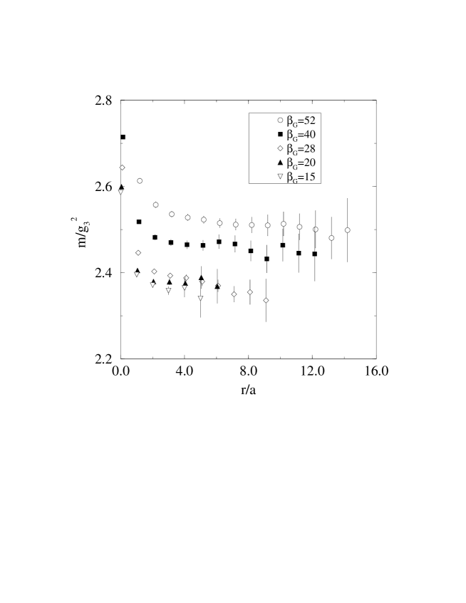
Figure 1: The local mass values, $m\,a=-\ln[G_{F}(n+1)/G_{F}(n)]$, from typical diagonalized operators at the different $\beta_{G}$’s. The masses have been converted to continuum units by multiplying the lattice values $m\,a$ with $\beta_{G}/6$.

We gathered statistics until the statistical errors of the local masses at their plateaux were well below 10%, which required between 500 and 4000 measurements, depending on the lattice size. The choice of lattice sizes was governed by the experience from SU(3) glueball measurements [16] as well as our previous SU(2) measurements [14]. We have also explicitly checked that finite volume effects are within the statistical errors at single values of $\beta_{G}$ (see Tables 1, 2), and then increased the volume with $\beta_{G}$, keeping it fixed in physical units.

4 Numerical results

Typical local mass values from the correlation functions in the case of SU(3) are shown in Fig. 1, exhibiting rather pronounced plateaux. The mass values quoted in this paper have been obtained by fitting an exponential to the optimal diagonalized correlation function, and choosing among various fitting ranges those giving the best values for $\chi^{2}/{\rm dof}$. The lengths of the fitting ranges are between 5 and 11 timeslices, and the $\chi^{2}$-values are between 0.5 – 1.5. We now discuss our results both for SU(2) and SU(3).

SU(2). Previously we carried out measurements for SU(2) with $\beta_{G}=9,12,16$ [14]. We have now added values closer to the continuum limit, $\beta_{G}=20,25$. The results are shown in Table 1 and in Fig. 2. As a continuum extrapolation we obtain $c_{2}=1.14(4)$. Note that we see the onset of a quadratic ${\cal O}(a^{2})$ term in $c_{2}$ on coarser lattices (the same is true also for SU(3)).

$\beta_{G}$	volume	$m\,a$	$m/g_{3}^{2}$	$c_{2}$
9	$30^{3}$	0.685(8)	1.54(2)	1.17(2)
12	$30^{2}\cdot 42$	0.517(7)	1.55(2)	1.13(2)
16	$42^{3}$	0.401(4)	1.60(2)	1.14(2)
	$54^{3}$	0.397(3)	1.59(2)	1.12(2)
20	$52^{3}$	0.327(5)	1.64(3)	1.13(3)
25	$64^{3}$	0.268(2)	1.68(2)	1.14(2)
$\infty$		–	–	1.14(4)

Table 1: The results for SU(2). The continuum extrapolation is from a linear fit to $\beta_{G}\geq 12$, with $\chi^{2}$/d.o.f. $=0.03$ (see Fig. 2).

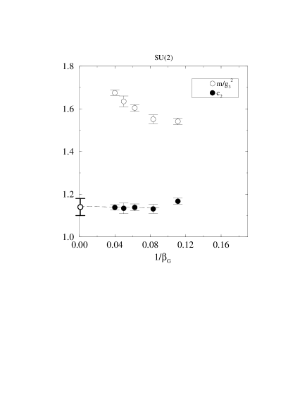
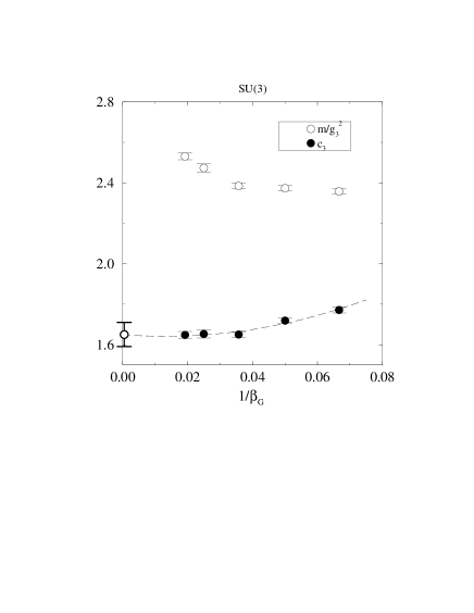
Figure 2: The results for SU(2) (left) and SU(3) (right). The continuum fits from Tables 1, 2 have also been shown. The ranges of $1/\beta_{G}$ on the $x$-axes have been chosen such that in lattice units, the masses have comparable values for SU(2) and SU(3).

SU(3). The results for SU(3) are shown in Table 2 and in Fig. 2. As for SU(2), the results show could scaling with $\beta_{G}$ after the removal of the logarithmic divergence. As a final continuum value we cite $c_{3}=1.65(6)$.

$\beta_{G}$	volume	$m\,a$	$m/g_{3}^{2}$	$c_{3}$
15	$18^{3}$	0.943(6)	2.36(2)	1.77(2)
20	$24^{3}$	0.712(4)	2.37(2)	1.72(2)
	$32^{3}$	0.707(5)	2.36(2)	1.70(2)
28	$32^{3}$	0.511(3)	2.38(2)	1.65(2)
40	$46^{3}$	0.371(3)	2.47(2)	1.65(2)
52	$60^{3}$	0.292(2)	2.53(2)	1.65(2)
$\infty$		–	–	1.65(6)

Table 2: The results for SU(3). The continuum extrapolation is from a quadratic fit to all the $\beta_{G}$-values, with $\chi^{2}$/d.o.f. $=1.25$. We use a quadratic fit for SU(3) since we are slightly farther from the continuum limit than for SU(2), see Fig. 2. A linear fit to $\beta_{G}\geq 28$ gives 1.65(5), with $\chi^{2}$/d.o.f. $=0.04$.

5 Discussion

Comparison with other measurements in 3d. Let us compare our results with those of previous studies. In [10], $c_{2},c_{3}$ were measured using operators $O\sim\epsilon_{3jk}{\rm Tr\,}A_{0}F_{jk}$ in the 3d SU(N) + adjoint Higgs theory, with the result $c_{2}=1.58(20)$, $c_{3}=2.46(15)$. In [14], we found the smaller result $c_{2}=1.06(4)$, using the field strength correlator in the pure 3d SU(2) theory as in this work. Adding two more lattice spacings to SU(2) and evaluating also SU(3), our present results are $c_{2}=$1.14(4), $c_{3}=$1.65(6). In conclusion, the values are considerably smaller than in [10]. However, there the system had multiple length scales, so it need not be a surprise that the result has some systematic uncertainties. Our present results scale quite well with $N$, a behaviour which is also observed for the glueball spectrum in SU(N) theories [16]. Furthermore, the bare numbers $m/g_{3}^{2}$ extracted from the Wilson lines exhibit the logarithmic divergence expected from lattice perturbation theory [5], adding further confidence to them.

The mass scales in units of temperature. We now proceed to estimate the numerical value of the Debye mass $m_{D}$ in units of $T$. For definiteness we take $N_{f}=0$, in which case $T_{c}/\Lambda_{\mbox{\scriptsize$\overline{\mbox{\rm MS}}$}}\approx 1.03(19)$ for SU(3) [17]. (Let us stress that the values of $c_{2},c_{3}$ as such do not depend on the fermionic content of the original 4d theory, and thus $c_{3}$ applies also to the physical QCD with $N_{f}\neq 0$.) At moderate temperatures of, say, $2T_{c}$, we then estimate that $g_{3}^{2}\approx 2.7T$ [9], and thus $m_{D}\sim 6T$. This estimate is of course somewhat rough, since terms of order $g^{3}T$ etc. have been neglected. However, the results in [10] suggest that these corrections should come with very small coefficients.

An important question for the construction of effective theories concerns the degree to which the Debye mass is perturbative, and the related issue of how well the electric ($\sim gT$) and magnetic ($\sim g^{2}T$) sectors are separated, once non-perturbative coefficients are taken into account. Even at very large temperatures, say, $T\sim 10^{4}T_{c}$ with a weaker coupling $g_{3}^{2}\approx 0.64T$, the correction ($\sim 1.1T$) is still larger than the leading term ($\sim 0.8T$). Both are of the same order ($\sim 0.7T$) only at $T\sim 10^{7}T_{c}$.

It is also interesting to compare with the masses in the magnetic sector, especially at low temperatures $T\sim 2T_{c}$. There the ordering of states according to the naive expectations is reversed. A purely magnetic excitation, the lightest glueball, has a mass $\sim 2.4g_{3}^{2}\sim 6T$ [16], making it as heavy as $m_{D}$. However, there is a lighter excitation with the same quantum numbers which then determines, e.g., the decay of the Polyakov loop. In the 3d SU(3) + adjoint Higgs theory, it is represented by the mass of the bound state $A_{0}^{a}A_{0}^{a}$, whose numerical value is about $\sim 3T$  [9, 18].

Comparison with measurements in 4d. All these numbers are in good qualitative agreement with those found with direct 4d simulations in [11]. In Table 5 of [11], $m(A_{1}^{++})\approx 2.60(4)T$ corresponds to the lightest mass in the $0^{++}$ channel [in the language of the 3d theory, to $m(A_{0}^{a}A_{0}^{a})\sim 3T$], while the ${\cal R}_{z}=-1$ [5, 11] mass $m(A_{1}^{-+})\approx 6.3(2)T$ should correspond to the lightest mass in the electric sector [in the language of the 3d theory, to $m_{D}$ as defined here, $\sim 6T$]. Since the 4d measurement of $m_{D}$ contains all orders in $g$ this agreement would indeed suggest corrections of order $g^{3}T$ and higher to be small.

Incidentally, we believe that, contrary to the suggestion in [11], the lightest masses measured in [11] do not correspond to the glueball masses measured in [16], but to scalar states involving $A_{0}$: the screening masses corresponding to static glueball correlators are heavier. Thus, close to $T_{c}$, the naive expectation that $A_{0}$ is heavy and decouples is completely unjustified (see also [8, 9, 20]). This should not be a surprise, since the actual transition is assumed to be driven by the Z($N$) symmetry related to the Polyakov line and $A_{0}$. At the same time, it is interesting to note that the higher lying glueball spectrum itself is expected to be relatively little affected by $A_{0}$ [19].

Conclusions. In conclusion, we have determined the non-perturbative contribution of the soft modes $\sim g^{2}T$ to the Debye mass in QCD and found it to be larger than the “leading” perturbative contributions for all reasonable temperatures. The approximate agreement between the values for the Debye mass as determined in this simulation and with the 4d measurement, further suggests that the ${\cal O}(g^{3}T)$ and higher corrections in the Debye mass are small even at relatively small temperatures, as already argued in [10]. The consistent picture emerging from our results, as well as from previous analytical work and simulations [8, 9, 10, 20], is that a dimensionally reduced theory gives a reliable description of correlation functions down to quite moderate temperatures $T\sim 2T_{c}$, when $A_{0}$ is kept in the action. However, at such temperatures $A_{0}$ may not be integrated out, but is in fact an essential constituent in the lightest physical degrees of freedom.

References

- [1] E. Shuryak, Zh. Eksp. Teor. Fiz. 74 (1978) 408 [Sov. Phys. JETP 47 (1978) 212]; J. Kapusta, Nucl. Phys. B 148 (1979) 461; D. Gross, R. Pisarski and L. Yaffe, Rev. Mod. Phys. 53 (1981) 43.
- [2] A.K. Rebhan, Phys. Rev. D 48 (1993) R3967 [hep-ph/9308232]; Nucl. Phys. B 430 (1994) 319 [hep-ph/9408262].
- [3] X.-N. Wang, Phys. Rep. 280 (1997) 287 [hep-ph/9605214].
- [4] G.D. Moore, hep-ph/9810313.
- [5] P. Arnold and L. Yaffe, Phys. Rev. D 52 (1995) 7208 [hep-ph/9508280].
- [6] P. Ginsparg, Nucl. Phys. B 170 (1980) 388; T. Appelquist and R. Pisarski, Phys. Rev. D 23 (1981) 2305.
- [7] K. Kajantie, M. Laine, K. Rummukainen and M. Shaposhnikov, Nucl. Phys. B 458 (1996) 90 [hep-ph/9508379]; Phys. Lett. B 423 (1998) 137 [hep-ph/9710538].
- [8] E. Braaten and A. Nieto, Phys. Rev. Lett. 76 (1996) 1417 [hep-ph/9508406]; Phys. Rev. D 53 (1996) 3421 [hep-ph/9510408]; A. Nieto, Int. J. Mod. Phys. A 12 (1997) 1431 [hep-ph/9612291].
- [9] K. Kajantie, M. Laine, K. Rummukainen and M. Shaposhnikov, Nucl. Phys. B 503 (1997) 357 [hep-ph/9704416].
- [10] K. Kajantie, M. Laine, J. Peisa, A. Rajantie, K. Rummukainen and M. Shaposhnikov, Phys. Rev. Lett. 79 (1997) 3130 [hep-ph/9708207].
- [11] S. Datta and S. Gupta, Nucl. Phys. B 534 (1998) 392 [hep-lat/9806034].
- [12] S. Bronoff and C.P. Korthals Altes, talk at Lattice ’98, Boulder, Colorado, 1998 [hep-lat/9808042]; Ph. Boucaud and C.P. Korthals Altes, talk at SEWM ’98, Copenhagen, Denmark, 1998 [hep-lat/9904006].
- [13] U.M. Heller, F. Karsch and J. Rank, Phys. Rev. D 57 (1998) 1438 [hep-lat/9710033]; A. Patkós, P. Petreczky and Z. Szep, Eur. Phys. J. C 5 (1998) 337 [hep-ph/9711263]; F. Karsch, M. Oevers and P. Petreczky, Phys. Lett. B 442 (1998) 291 [hep-lat/9807035].
- [14] M. Laine and O. Philipsen, Nucl. Phys. B 523 (1998) 267 [hep-lat/9711022].
- [15] O. Philipsen and H. Wittig, Phys. Rev. Lett. 81 (1998) 4056 [hep-lat/9807020]; Phys. Lett. B 451 (1999) 146 [hep-lat/9902003]; F. Knechtli and R. Sommer, Phys. Lett. B 440 (1998) 345 [hep-lat/9807022]; P. Stephenson, hep-lat/9902002.
- [16] M. Teper, Phys. Rev. D 59 (1999) 014512 [hep-lat/9804008].
- [17] J. Fingberg, U. Heller and F. Karsch, Nucl. Phys. B 392 (1993) 493 [hep-lat/9208012].
- [18] K. Kajantie, M. Laine, A. Rajantie, K. Rummukainen and M. Tsypin, JHEP 11 (1998) 011 [hep-lat/9811004].
- [19] O. Philipsen, M. Teper and H. Wittig, Nucl. Phys. B 469 (1996) 445 [hep-lat/9602006]; Nucl. Phys. B 528 (1998) 379 [hep-lat/9709145]; E.M. Ilgenfritz, A. Schiller and C. Strecha, Eur. Phys. J. C 8 (1999) 135 [hep-lat/9807023]; O. Philipsen, talk at SEWM ’98, Copenhagen, Denmark, 1998 [hep-ph/9902376].
- [20] T. Reisz, Z. Phys. C 53 (1992) 169; L. Kärkkäinen, P. Lacock, D.E. Miller, B. Petersson and T. Reisz, Phys. Lett. B 282 (1992) 121; Nucl. Phys. B 418 (1994) 3 [hep-lat/9310014]; L. Kärkkäinen, P. Lacock, B. Petersson and T. Reisz, Nucl. Phys. B 395 (1993) 733.