BI-TP 99/02
April 1999

Determination of Anisotropy Coefficients
for SU(3) Gauge Actions from the
Integral and Matching Methods
J. Engels^a, F. Karsch^a and T. Scheideler^b,

^aFakultät für Physik, Universität Bielefeld, D-33615 Bielefeld, Germany

^bDepartment of Physics, P.O.Box 9, 00014 University of Helsinki, Finland

Abstract

We use two non-perturbative methods to obtain the anisotropy derivatives of the coupling constants (the anisotropy coefficients) of $SU(3)$ lattice gauge theory. These coefficients appear in the derivative formulae for the energy density and the pressure. We calculate them for the standard Wilson and two improved actions, the $(2\times 2)$ and the Square Symanzik action. Both methods lead for all investigated actions to compatible results which are clearly different from their known asymptotic perturbative limits. With increasing $\beta$ the limits are however approached in all cases. Our findings strongly support the equivalence of the integral and derivative methods for the calculation of energy density and pressure.

1 Introduction

For the investigation of the phase transition from ordinary hadronic matter to the quark gluon plasma and the approach of the plasma to its high temperature limit the calculation of the energy density $\epsilon$ and the pressure $p$ is of central importance. These observables are defined as derivatives of the partition function $Z$ with respect to temperature $T$ and volume $V$

$$\epsilon=-{1\over V}{\partial\ln Z\over\partial(1/T)}~{},\quad\quad p=T{\partial\ln Z\over\partial V}~{}.$$ (1.1)

In the lattice formulation of QCD the temperature and the volume therefore have to be independent variables. On a lattice with a fixed number of points $N_{\sigma}$  in each spatial direction, and $N_{\tau}$  points in the temporal direction, this is achieved by choosing corresponding independent lattice spacings $a_{\sigma}$ and $a_{\tau}$ so that

$$V=(N_{\sigma}a_{\sigma})^{3}\quad{\rm and}\quad T^{-1}=N_{\tau}a_{\tau}~{}.$$ (1.2)

As a consequence two different coupling constants have to be introduced for the spatial and temporal contributions to the action. For $SU(N_{c})$ lattice gauge theory we consider actions of the following form

$$S=\beta_{\sigma}\sum_{x,\mu<\nu<4}S_{\mu\nu}(x)+\beta_{\tau}\sum_{x,\mu<4}S_{\mu 4}(x)~{},$$ (1.3)

where $S_{\mu\nu}(x)$ is a generalized plaquette in the $(\mu,\nu)-$plane. Generalized plaquette expectation values are then defined by

$$P_{\sigma} = {1\over 3N_{\sigma}^{3}N_{\tau}}\big{<}\sum_{x,\mu<\nu<4}S_{\mu\nu}(x)\big{>}$$ (1.4)

$$P_{\tau} = {1\over 3N_{\sigma}^{3}N_{\tau}}\langle\sum_{x,\mu<4}S_{\mu 4}(x)\rangle~{}.$$ (1.5)

The couplings $\beta_{\sigma,\tau}$ may be rewritten in terms of the coupling constants $g^{2}_{\sigma,\tau}$ as

$$\beta_{\sigma}={2N_{c}\over g^{2}_{\sigma}}\cdot{1\over\xi}\quad{\rm and}\quad\beta_{\tau}={2N_{c}\over g^{2}_{\tau}}\cdot\xi~{}.$$ (1.6)

Here $\xi=a_{\sigma}/a_{\tau}$ is the anisotropy. One may also express the couplings with the bare anisotropy $\gamma$ and a common coupling $\beta$ through [1]

$$\beta=\sqrt{\beta_{\sigma}\beta_{\tau}}={2N_{c}\over g^{2}}~{},\quad\gamma=\sqrt{{\beta_{\tau}\over\beta_{\sigma}}}=\xi\cdot{g_{\sigma}\over g_{\tau}}~{},$$ (1.7)

or equivalently

$$\beta_{\sigma}={\beta\over\gamma}~{},\quad\beta_{\tau}=\beta\gamma~{}.$$ (1.8)

The couplings depend on $a_{\sigma}$ and $a_{\tau}$, or, alternatively, on $a_{\sigma}$ and $\xi$. Following ref. [2] we adopt the latter two as independent variables. The energy density and pressure are then

$$\epsilon=-{T\over V}\Big{<}\xi{\partial S\over\partial\xi}\Big{>}~{},\quad\quad\epsilon-3p={T\over V}\Big{<}a_{\sigma}{\partial S\over\partial a_{\sigma}}\Big{>}~{}.$$ (1.9)

Obviously, the energy density contains now terms, which are proportional to derivatives with respect to the anisotropy $\xi$, because

$$\xi{\partial\beta_{\sigma}\over\partial\xi}\! = \!-\beta_{\sigma}+2N_{c}{\partial g^{-2}_{\sigma}\over\partial\xi}~{},$$ (1.10)

$$\xi{\partial\beta_{\tau}\over\partial\xi}\! = \!\beta_{\tau}+2N_{c}\xi^{2}{\partial g^{-2}_{\tau}\over\partial\xi}~{}.$$ (1.11)

After taking the derivatives one can evaluate the expressions on isotropic lattices. At $\xi=1$ we have

$$\gamma=1~{},\quad g_{\sigma}=g_{\tau}=g~{},\quad a_{\sigma}=a_{\tau}=a~{},$$ (1.12)

and the relation for the $\beta-$function [3]

$$a{dg^{-2}\over da}=-2\left({\partial g^{-2}_{\sigma}\over\partial\xi}+{\partial g^{-2}_{\tau}\over\partial\xi}\right)_{\xi=1}~{}.$$ (1.13)

Energy density and pressure are now conveniently combined in the two equations

$${\epsilon+p\over T^{4}}\!\! = \!\!8N_{c}N_{\tau}^{4}g^{-2}\left[1-{g^{2}\over 2}\left({\partial g^{-2}_{\sigma}\over\partial\xi}-{\partial g^{-2}_{\tau}\over\partial\xi}\right)_{\xi=1}\right](P_{\sigma}-P_{\tau})~{},$$ (1.14)

$${\epsilon-3p\over T^{4}}\!\! = \!\!12N_{c}N_{\tau}^{4}\left({\partial g^{-2}_{\sigma}\over\partial\xi}+{\partial g^{-2}_{\tau}\over\partial\xi}\right)_{\xi=1}[2P_{0}-(P_{\sigma}+P_{\tau})]~{}.$$ (1.15)

Here $P_{0}$ denotes a generalized plaquette on a symmetric ($T=0$) lattice. Its inclusion normalizes both $\epsilon$ and $p$ to zero at $T=0$.

We define the anisotropy coefficients $c_{\sigma,\tau}$ as follows

$$c_{\sigma,\tau}(a)\equiv\left({\partial g^{-2}_{\sigma,\tau}\over\partial\xi}\right)_{\xi=1}~{}.$$ (1.16)

In the weak coupling limit, they are related to the derivatives of the anisotropic parts of the couplings

$$g^{-2}_{\sigma,\tau}(a,\xi)=g^{-2}(a)+c^{w}_{\sigma,\tau}(\xi)+O(g^{2})~{},$$ (1.17)

by

$$c_{\sigma,\tau}(0)=\left({\partial c^{w}_{\sigma,\tau}(\xi)\over\partial\xi}\right)_{\xi=1}.$$ (1.18)

The quantities $c^{w}_{\sigma,\tau}(\xi)$ were calculated in ref.[3] for the Wilson action perturbatively. For the difference one obtains

$$c_{\sigma}(0)-c_{\tau}(0)={N_{c}^{2}-1\over N_{c}}\cdot 0.146711-N_{c}\cdot 0.019228~{},$$ (1.19)

and, from the renormalization group equation and eq. (1.13)

$$c_{\sigma}(0)+c_{\tau}(0)=b_{0}={11N_{c}\over 48\pi^{2}}~{}.$$ (1.20)

These perturbatively calculated anisotropy coefficients were used in early finite temperature lattice calculations. In $SU(3)$ gauge theory, however, this led to unphysical behaviour of the pressure: it could become negative and at the critical point a gap in $p$ was observed [4, 5]. A second, rather important consequence of taking only the perturbative coefficients is the rapid approach of $\epsilon$ and $p$ to their respective ideal gas limits soon after the transition, though the limits themselves are independent of $c_{\sigma,\tau}$. The actual form of the approach is of course dependent on the residual interaction in the quark gluon plasma, and therefore of physical relevance.

In ref. [6] an alternative method for the calculation of energy density and pressure was proposed, which is now in common use. Here the pressure is obtained without the anisotropy coefficients from an integral over plaquettes. In order to be consistent, the integral method should be equivalent to the use of non-perturbative anisotropy coefficients, i.e. the corresponding values for $c_{\sigma,\tau}$ should be essentially independent on finite size and cut-off effects. First results in ref.[7] showed however considerable cut-off effects for the Wilson action. To clarify the situation, we started [8] a non-perturbative calculation of the coefficients with the matching method, which we want to complete in this paper.

In the following section we discuss the integral method in some more detail as in [7] and [8] and apply it to the Wilson action. The matching method is described and applied to the same action in section 3. For comparison we determine in section 4 the anisotropy coefficients as well for two improved actions, the $(2\times 2)$ and the Square Symanzik action [9]. We close with a summary and the conclusions.

2 The integral method

For large homogeneous systems with isotropic interactions, the volume derivative in the pressure formula (1.1) may be replaced by a volume division. The pressure and the free energy density are then related by

$$p=-f={T\over V}\ln Z~{}.$$ (2.1)

Instead of calculating ln$Z$ directly, one may take advantage of the relation

$${\partial\ln Z\over\partial\beta}=-\Big{<}{\partial S\over\partial\beta}\Big{>}~{},$$ (2.2)

and integrate the measured expectation value over a $\beta-$range. For $\xi=1$ we obtain then

$${p\over T^{4}}=\left.{p\over T^{4}}\right|_{\beta_{0}}+\int\limits_{\beta_{0}}^{\beta}d\beta^{\prime}[2P_{0}-(P_{\sigma}+P_{\tau})]~{}.$$ (2.3)

As in eqs. (1.14) and (1.15), the inclusion of the $P_{0}-$term serves to normalize $p$ at $T=0$ to zero. Obviously, the last equation will lead to a continuous pressure, even if there is a gap in the plaquettes at the critical point. The energy density is found from

$${\epsilon-3p\over T^{4}}=-6N_{c}N_{\tau}^{4}a{dg^{-2}\over da}[2P_{0}-(P_{\sigma}+P_{\tau})]~{},$$ (2.4)

by just adding $3p/T^{4}$. Here we have replaced the sum of the coefficients by the $\beta-$function. This function and/or $a=a(g^{2})$ have to be known non-perturbatively, not only to evaluate the last equation, but also to determine the temperature $T=1/N_{\tau}a$ on fixed $N_{\tau}-$lattices at any given coupling. Parametrizations of the $\beta-$function for the $SU(3)$ Wilson action have been derived by several groups [7, 10, 11]. They are rather similar above $\beta=5.9$, but below this value they differ from each other. Probably this is due to the transition from the weak coupling to the strong coupling regime.

2.1 The high temperature limit

The two methods for the calculation of $\epsilon$ and $p$ on the lattice suffer from cut-off effects, especially for small $N_{\tau}-$values. Though these cut-off effects are of similar size, there is a non-negligible difference. For the same method, the high temperature limits of $\epsilon$ and $p$ have the same cut-off dependencies, because in both cases the same formula for $(\epsilon-3p)/T^{4}$ is used and

$$(\epsilon-3p)/T^{4}=O(g^{4})~{}.$$ (2.5)

$N_{\tau}$	$R_{D}$	$R_{I}$	$r=R_{D}/R_{I}$
4	1.4952	1.3778	1.0852
6	1.1816	1.1323	1.0435
8	1.0867	1.0659	1.0195

Table 1: The ratios $R(N_{\tau})=\epsilon(N_{\tau})/\epsilon_{SB}=p(N_{\tau})/p_{SB}$ for the Wilson action calculated with the derivative ($R_{D}$) and the integral methods ($R_{I}$).

However, as different methods are based on the evaluation of different operators, which have different cut-off dependencies, the high$-T$ limit derived in different approaches leads also to distinct cut-off dependencies. In the derivative method the high temperature limit is derived from the lowest order of the $g^{2}-$expansion of the energy density ($\xi=1$)

$${\epsilon\over T^{4}} = 6N_{c}N_{\tau}^{4}g^{-2}(P_{\sigma}-P_{\tau})+O(g^{2})~{},$$ (2.6)

$$= {3\over 2}(N_{c}^{2}-1)N_{\tau}^{4}(P_{\sigma}^{(2)}-P_{\tau}^{(2)})+O(g^{2})~{}.$$ (2.7)

The quantities $P_{\sigma,\tau}^{(2)}$ are the corresponding expansion coefficients of the generalized plaquette expectation values

$$P_{\sigma,\tau}=g^{2}{N_{c}^{2}-1\over 4N_{c}}P_{\sigma,\tau}^{(2)}+O(g^{2})~{}.$$ (2.8)

For the Wilson action one obtains the following deviation of the energy density, $\epsilon(N_{\tau})$, in the high $T$ limit from the continuum result, $\epsilon_{SB}$ [12]

$$R_{D}={\epsilon(N_{\tau})\over\epsilon_{SB}}=1+{10\over 21}\left({\pi\over N_{\tau}}\right)^{2}+{2\over 5}\left({\pi\over N_{\tau}}\right)^{4}+O\left({1\over N_{\tau}^{6}}\right)~{}.$$ (2.9)

If the integral method is used, the calculation of the high temperature limit starts from eq.(2.1) and the lowest order term of ln$Z$. Here the $T=0$ subtraction has to be done explicitly. With the Wilson action one arrives at

$$R_{I}={f(N_{\tau})\over f_{SB}}=1+{8\over 21}\left({\pi\over N_{\tau}}\right)^{2}+{5\over 21}\left({\pi\over N_{\tau}}\right)^{4}+O\left({1\over N_{\tau}^{6}}\right)~{},$$ (2.10)

where of course $\epsilon_{SB}=-3f_{SB}$. The full $1/N_{\tau}^{2}-$expansions can be calculated numerically. In Table 1 we list them for the two methods in the case of the Wilson action and $N_{\tau}=4,6,8\,$. We show also the ratio $r$ between the two high temperature limits. We stress that this difference, which expresses itself in the ratio $r$, will play a crucial role in the discussion of the anisotropy coefficients presented in the following sections.

2.2 Determination of the anisotropy coefficients

As mentioned already in the introduction, the integral method implies the use of non-perturbative anisotropy coefficients. We can determine them by comparing the pressure formulae from the two different approaches

$$\left({p\over T^{4}}\right)_{D}=r\cdot\left({p\over T^{4}}\right)_{I}~{},$$ (2.11)

and by exploiting the $\beta-$function relation, eq.(1.13). In the pressure equation (2.11) we have inserted the factor $r$ as a compensation for the differing cut-off effects. In principle, $r=r(g^{2})\,$. We approximate $r$ by its value at $g^{2}=0$ (Table 1). From eqs.(1.14) and (1.15) we obtain

$$\left({p\over T^{4}}\right)_{D}=N_{c}N_{\tau}^{4}\left[\left(2g^{-2}-(c_{\sigma}-c_{\tau})\right)(P_{\sigma}-P_{\tau})-3(c_{\sigma}+c_{\tau})\Bigl{(}2P_{0}-(P_{\sigma}+P_{\tau})\Bigr{)}\right]~{},$$ (2.12)

and therefore

$$\!\!c_{\sigma}\!\!\! = \!\!\!g^{-2}-{a\over 4}{dg^{-2}\over da}$$ (2.13)

$$\!\!\!+{1\over\ P_{\sigma}-P_{\tau}}\left[-{r\over 2N_{c}N_{\tau}^{4}}\left({p\over T^{4}}\right)_{I}+{3a\over 4}{dg^{-2}\over da}\Bigl{(}2P_{0}-(P_{\sigma}+P_{\tau})\Bigr{)}\right]~{},$$

$$\!\!c_{\tau}\!\!\! = \!\!\!-c_{\sigma}-{a\over 2}{dg^{-2}\over da}~{}.$$ (2.14)

In the following we discuss the behaviour of $c_{\sigma}$. The behaviour of $c_{\tau}$ is similar, because both coeffcients are related by the smooth $\beta-$function. It is clear, that the numerical determination of the coefficients becomes problematic below the transition point, because there both the pressure and the plaquette differences are small. Indeed, this is seen in Fig. 2, where we show $c_{\sigma}$ for the $SU(3)$ Wilson action as obtained from eq. (2.13) on $N_{\tau}=4,6,8-$lattices using interpolations of the $[P_{\sigma}-P_{\tau}]$ and $[P_{0}-(P_{\sigma}+P_{\tau})/2]-$data of ref. [7]. Apart from the close vicinity of the critical

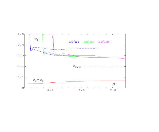
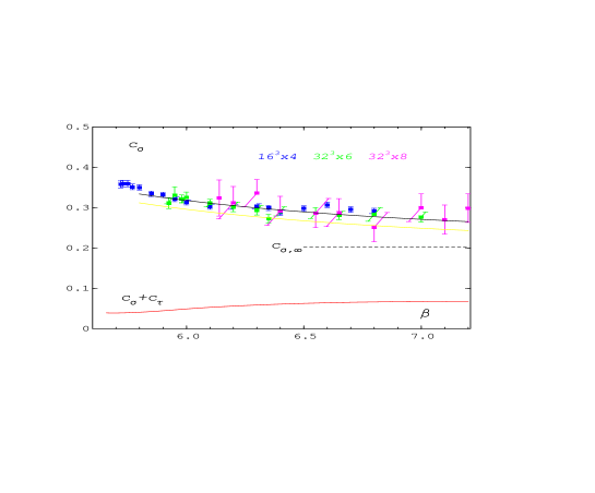
Figure 1: The coefficient $c_{\sigma}$ for the $SU(3)$ Wilson action from plaquette interpolations. The dashed curve is without cut-off corrections from ref. [8]. Also shown is the perturbative result for $\beta\rightarrow\infty\,$, $c_{\sigma,\infty}$ and the sum $c_{\sigma}+c_{\tau}$.

Figure 2: The coefficient $c_{\sigma}$ for the $SU(3)$ Wilson action with errors coming from the plaquette data . The solid curve is the fit, eq. (2.15), the yellow line a corresponding fit to data (not shown), which one obtains if $p/T^{4}(\beta_{0}=5.65,N_{\tau}=4)=0.05$ .

$\beta-$values the results for different $N_{\tau}$ are consistent with each other. For comparison we show also the previous result for $N_{\tau}=4$ from ref. [8], where the difference in the cut-off effects of the two methods was not taken into account, that is $r=1$ was used. Obviously the influence of the $r-$factor is important. Moreover it leads to slightly lower results for $c_{\sigma}$, though, as before, there remains a substantial deviation from the asymptotic value $c_{\sigma,\infty}\equiv c_{\sigma}(0)$ from eqs. (1.19) and (1.20).

It is difficult to estimate all possible error sources in the calculation of $c_{\sigma}$, as for example that of the parametrization of the $\beta-$function. The major errors are certainly due to the errors in the plaquette expectation values. In Fig. 2 we present the results including these errors, but omitting the respective critical regions. We can summarize these data with a simple Padé fit of the form

$$c_{\sigma}=c_{\sigma,\infty}{1+d_{1}g^{2}+d_{2}g^{4}\over 1+d_{0}g^{2}}~{},$$ (2.15)

where $d_{0}=-0.64907,~{}d_{1}=-0.61630,~{}d_{2}=0.16965$ .

A further source of errors is the result for $(p/T^{4})_{I}$ . Whereas the integration itself contributes only a negligible error, the size of the pressure at the lower integration boundary $\beta_{0}$ is unknown. We have identified $\beta_{0}$ with the point where the integrand $[P_{0}-(P_{\sigma}+P_{\tau})/2]$ is disappearing and assumed, as usual, that there $p/T^{4}$ is zero. This may be not true. In order to assess the effect of a non-zero pressure contribution we have repeated our calculation with a test value $p/T^{4}=0.05$ at $\beta_{0}=5.65,T_{0}/T_{c}=0.917$ for $N_{\tau}=4$. As a result the value of $c_{\sigma}$ is diminished by 0.022 in the whole $\beta-$range considered. The same shift in $c_{\sigma}$ is observed also for $N_{\tau}=6$ and 8. For comparison we have plotted in Fig. 2 a fit of the form (2.15) to the shifted data as well. Here we find $d_{0}=-0.60983,~{}d_{1}=-0.78889,~{}d_{2}=0.36164$ .

Some insight into the question of the pressure size below the transition is gained from the behaviours of the plaquette differences around $T_{c}$ in $SU(3)$ and $SU(2)$. In Fig. 3 we compare them to each other. The main difference between the two gauge groups is evidently arising from the fact, that the respective phase transitions are of different order. Also, there is no doubt, that in $SU(2)$ the pressure is non-zero well below $T_{c}$.

As we have seen in $SU(3)$ the inclusion of the cut-off factor $r$ considerably lowers the $N_{\tau}=4-$result for $c_{\sigma}\,$. In $SU(2)$ the values which were previously [14] determined

Figure 3: The plaquette differences in the vicinity of the deconfinement transition for $SU(2)$ and $SU(3)$ on $N_{\tau}=4-$lattices. The $SU(2)-$data are from ref. [13].

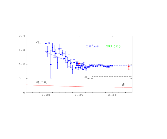
Figure 4: The coefficient $c_{\sigma}$ for the $SU(2)$ Wilson action with errors coming from the plaquette data and $r=1.0852$. The dashed curve $(r=1)$ and the sum $c_{\sigma}+c_{\tau}$ are from ref. [14], the red points from ref. [15]. Also shown is $c_{\sigma,\infty}$ .

for $c_{\sigma}$ with the integral method and $r=1$ are well in accord with points measured in an independent way at $\beta=2.30$ and $\beta=2.375$ by Ejiri et al. [15]. One has to check then, whether this agreement is lost if the correct $r$ is taken into account. We do this by using the new high precision $SU(2)$ data of ref. [13], already shown in Fig. 3, the $\beta-$function of ref. [14] and the $r-$value from Table 1. The resulting $c_{\sigma}$ is plotted in Fig. 4. We find only a small change in this $\beta-$range, the result is lowered at $\beta=2.30$ by 0.0067 and at $\beta=2.35$ by 0.0142 . The reason for this is, that up to $\beta=2.35$ the difference $[P_{0}-(P_{\sigma}+P_{\tau})/2]$ is still large and only at higher couplings the pressure term with the factor $r$ is dominating in eq. (2.13) . We expect therefore a stronger decrease at higher $\beta-$values.

3 The matching method

This method was first used by Burgers et al. [1] to measure the anisotropy $\xi$ as a function of the bare anisotropy $\gamma$ on anisotropic lattices. With this information one may as well determine the anisotropy coefficients. Consider the couplings

$$g_{\sigma}^{-2}={\beta\over 2N_{c}}{\xi\over\gamma}\quad,\quad g_{\tau}^{-2}={\beta\over 2N_{c}}{\gamma\over\xi}~{},$$ (3.1)

and their derivatives with respect to the anisotropy $\xi$

$${\partial g^{-2}_{\sigma}\over\partial\xi}\!\! = \!\!g^{-2}_{\sigma}\left(~{}~{}{1\over\xi}+{\partial\ln\beta\over\partial\xi}-{\partial\ln\gamma\over\partial\xi}\right)~{},$$ (3.2)

$${\partial g^{-2}_{\tau}\over\partial\xi}\!\! = \!\!g^{-2}_{\tau}\left(-{1\over\xi}+{\partial\ln\beta\over\partial\xi}+{\partial\ln\gamma\over\partial\xi}\right)~{}.$$ (3.3)

At $\xi=1$ we may apply eq. (1.12) to find the difference

$$c_{\sigma}-c_{\tau}=2g^{-2}\left(1-{\partial\gamma\over\partial\xi}\right)_{\xi=1}~{},$$ (3.4)

and, using eq. (1.13), we obtain

$$c_{\sigma,\tau}=\pm g^{-2}\left(1-{\partial\gamma\over\partial\xi}\right)_{\xi=1}-{a\over 4}{dg^{-2}\over da}~{}.$$ (3.5)

A measurement of the function $\xi(\gamma)$ in the neighbourhood of $\xi=1$ will therefore enable us to calculate the anisotropy coefficients, once we know the $\beta-$function. In principle, the anisotropy $\xi$ may be determined with two measurements of a physical observable which depends on a distance, which can be chosen in a spatial or in the temporal direction. At the same physical distance the expectation values have to be the same and thereby fix the anisotropy. This is the idea of matching.

3.1 Matching of Wilson loop ratios

Suitable quantities for the matching process are obtained from Wilson loops of size $n_{1}\times n_{2}$ (in lattice units) . The Wilson loops are related to the heavy quark potential

$$W(x_{1},x_{2})\sim\exp[-x_{1}V_{l}(x_{2})]~{},$$ (3.6)

for $x_{1}\rightarrow\infty\,$. Here, $x_{i}=n_{i}a_{i}$. The potential $V_{l}$ differs from the continuum potential $V$ by a term $V_{0}$, the self-energy of the heavy quarks, which is dependent on lattice spacing, but independent of $x_{2}$ [16]. The natural way to proceed then is to build ratios of Wilson loops, which depend only on $V_{l}(x_{2})$ for large $x_{1}$. We use the following ratios

$$R_{1}(n_{1},n_{2}) = {W(x_{1}+a_{1},x_{2})\over W(x_{1},x_{2})}~{};$$ (3.7)

$$R_{2}(n_{1},n_{2}) = {W(x_{1}+2a_{1},x_{2})\,W(x_{1}+a_{1},x_{2})\over W(x_{1},x_{2})^{2}}~{}.$$ (3.8)

On an anisotropic lattice there are two different types of loops : space-space ($W_{\sigma\sigma}$) and space-time ($W_{\sigma\tau}$) Wilson loops. The corresponding ratios $R_{\sigma}$ and $R_{\tau}$ are measuring the same potential $V(x_{2})$, if the matching condition for the physical distance

$$x_{2}=y=t\quad{\rm or}\quad n_{t}=\xi n_{y}~{},$$ (3.9)

is fulfilled, apart from an $n-$independent factor $k=k_{\sigma\sigma}/k_{\sigma\tau}\,$, which is due to the dependence of $V_{0}$ on $a_{\sigma}$ and $\xi$

$$R_{\sigma}(n_{x},n_{y})=k\cdot R_{\tau}(n_{x},n_{t}=\xi n_{y})~{}.$$ (3.10)

At $\xi=1$ the factor $k$ is of course $1\,$. We do not implement any smearing for our Wilson loops, because then space and time links would have to be smeared by the same amount in physical units. However, in order to enhance the accuray of the Wilson loop measurements we are using the fast link integration technique of de Forcrand and Roiesnel [17] wherever this is feasible. It cannot be done for loops with an $n_{i}=1$ and at loop edges. In applying this algorithm we are saving in addition half of the computer time by taking advantage of the fact that the necessary link contour integrals are real and can as well be obtained from a half contour in the complex plane.

For the Wilson action simulations were performed at four $\beta-$values: 5.4, 5.7, 6.3 and 7.2 using a $16^{4}$ lattice for $\gamma\in[0.92,1.08]$, a $16^{3}\times 32$ lattice for $\gamma\in[1.1,2.0]$ and a $16^{3}\times 48$ lattice for $\gamma=3.0$. The Wilson loops were calculated after every fourth sweep through the lattice, where a sweep consisted of one heatbath update succeeded by four overrelaxation steps. The integrated autocorrelation times which one finds then are increasing with increasing $\beta$ from 0.5, 1.5, 3.0 to over 3.0 for $\beta=7.2\,$. On the average we took 5000-7000 measurements for $\beta=5.4-6.3$ and 600 for $\beta=7.2\,$. Generally, for the same number of measurements, the relative error of a Wilson loop increases with the size of its area. The increase itself is much steeper at lower $\beta-$values than at higher ones. Larger area Wilson loops are therefore only included in the matching procedure for the higher $\beta-$values. In Fig. 5 we show a typical example of this behaviour. The difference in accuracy between link integrated and plain loops is clearly seen in the plot.

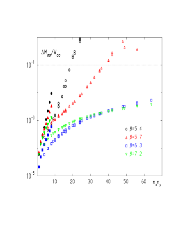
Figure 5: The relative errors of spatial Wilson loops as a function of their area at $\gamma=1.06\,$. Open symbols show the errors of link integrated loops, filled symbols those of not integrated ones.

After measuring the Wilson loops at a fixed value of $\beta$ and $\gamma$, we compute the ratios $R_{\sigma}$ and $R_{\tau}\,$. For $\gamma>1$ we connect the timelike ratios $R_{\tau}$ with spline interpolations. In order to improve the interpolations we include as well the ratios with $n_{t}=1\,$. The spatial ratios $R_{\sigma}$ are then shifted in $n_{y}$ by a factor $\xi$ and in height

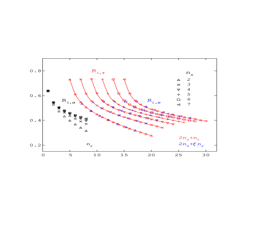
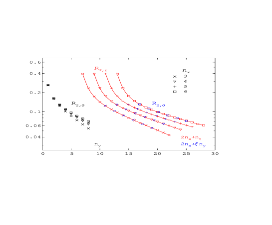
Figure 6: The ratios $R_{1,\tau}(n_{x},n_{t})$ at $\beta=6.3$ and $\gamma=1.5$ for fixed $n_{x}=2,...,7$ plotted vs. $2n_{x}+n_{t}$ and connected by splines. The ratios $R_{1,\sigma}(n_{x},n_{y})$ are once plotted vs. $n_{y}$ and also shifted, that is vs. $2n_{x}+\xi n_{y}$, with $\xi=1.63\,$.

Figure 7: The ratios $R_{2,\tau}(n_{x},n_{t})$ at $\beta=6.3$ and $\gamma=1.5$ for fixed $n_{x}=3,...,6$ plotted vs. $2n_{x}+n_{t}$ and connected by splines. The ratios $R_{2,\sigma}(n_{x},n_{y})$ are once plotted vs. $n_{y}$ and also shifted, that is vs. $2n_{x}+\xi n_{y}$, with $\xi=1.63\,$.

by a factor $k$ such that the sum of the squared deviation ($\chi^{2}$) of the shifted $R_{\sigma}-$values from the respective $R_{\tau}-$interpolations becomes minimal. For $\gamma<1$ the roles of $R_{\sigma}$ and $R_{\tau}$ are interchanged. The fitting is done for all ratios with $n_{x}\geq m_{x}$ and $n_{y}\geq m_{y}$ at the same time, with suitably chosen minimal values $m_{x}$ and $m_{y}$. In so far our procedure differs from the matching prescription of Klassen [18], who matches single ratios and looks for a possible plateau of shift values. In Figs. 7 and 7 we show matching examples at $\beta=6.3$ and $\gamma=1.5$ for the ratios $R_{1}$ and $R_{2}\,$. The matching in Fig. 7 is optimized for $m_{x}=m_{y}=2\,$, in Fig. 7 for $m_{x}=m_{y}=3\,$. Both lead to the same value $\xi=1.63$ for the anisotropy. For $R_{1}$ we find $k=1.01$ and $k=1.02$ for $R_{2}\,$, that is $k$ is always very close to one. One may as well perform fits, as Klassen[18] does, with fixed $k=1$. The corresponding $\chi^{2}$ is then considerably larger, the value for $\xi$ increases slightly. We shall come back to this point again.

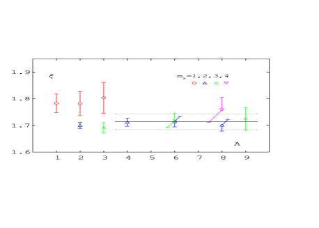
Figure 8: The result for $\xi$ from the matching of $R_{1}$ at $\beta=5.7$ and $\gamma=1.5$ as a function of $A=m_{x}m_{y}\,$. In the matching all ratios with $n_{x}\geq m_{x}$ and $n_{y}\geq m_{y}$ were taken into account. The lines show the final result with an error band.

As has been mentioned already, we have included only ratios in the matching process which are built from Wilson loops with at least minimal extensions $m_{x}$ and $m_{y}\,$. This has been done for two reasons. Once, $x_{1}$ should anyhow not be too small(see eq. (3.6)) and second, Wilson loops with a single link on one side cannot be link integrated and are therefore less accurate. That is why we disregard ratios with $n_{x}=1$ and/or $n_{y}=1$ in the final analysis. The influence of the chosen minimal values on the matching result for $\xi$ is demonstrated in Fig. 8 for $R_{1}$ at $\beta=5.7$ and $\gamma=1.5\,$. We observe, that apart from the $m_{x}=1$ data all other measurements for $\xi$ are consistent with each other.

3.2 Results for $c_{\sigma,\tau}$ from matching

In order to obtain the anisotropy coefficients we measure now the function $\xi(\gamma)$ in the neighbourhood of $\gamma=1$ with the aim of determining the derivative $(\partial\xi/\partial\gamma)_{\xi=1}\,$. In principle one would choose $\gamma$ rather close to one. However, the difference between spatial and temporal Wilson loops becomes then very small as well and the matching will be inexact. Fortunately, it turns out, that $\xi$ is linear in $\gamma$ in a wide range around $\gamma=1$ at all $\beta-$values. A successful strategy is therefore to measure the Wilson loops with high precision at not too many $\gamma-$values to determine the slope of $\xi(\gamma)\,$. In Fig. 9 we show as an example the function $\xi(\gamma)$ for the Wilson action at $\beta=5.7$ as obtained from the matching of $R_{1}$ with $m_{x}=2,m_{y}=3$, together with a linear fit to the data points.

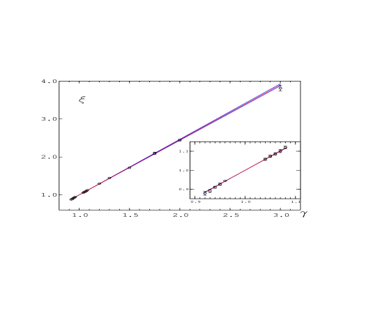
Figure 9: The anisotropy $\xi(\gamma)$ at $\beta=5.7$ as determined from the ratio $R_{1}$ with $m_{x}=2,m_{y}=3$. The red lines are from a linear fit in $\gamma$, the blue lines show the error band .

As in the last section, we use now the $\beta-$function of ref. [7] to deduce the anisotropy coefficients from the measured derivative $(\partial\xi/\partial\gamma)_{\xi=1}\,$. The corresponding

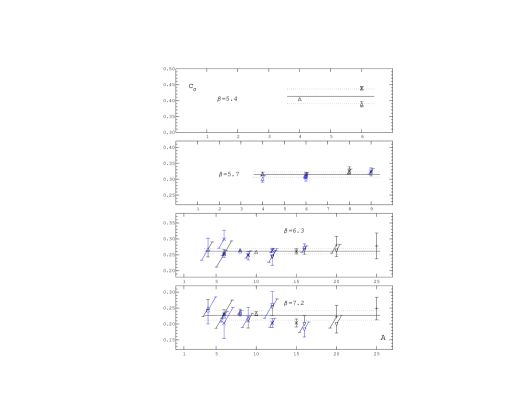
Figure 10: The anisotropy coefficient $c_{\sigma}$ of the Wilson action from the matching of $R_{1}$ (black) and $R_{2}$ (blue points) as a function of $A=m_{x}m_{y}$ for $\beta=5.4,\,5.7,\,6.3,\,$ and $7.2\,$. Points with $m_{x}=2,3,4,5$ are denoted by $\bigtriangleup,\times,\bigtriangledown,+\,$, respectively.

results for $c_{\sigma}$ are shown in Fig. 10 as a function of the minimal area $A=m_{x}m_{y}$ of the Wilson loops, which were included in the ratio-matching. The data for $\beta=5.4$ are somewhat problematic in several respects and can only serve as an indication for the true value. As demonstrated already in Fig. 5 too large Wilson loops cannot be included in the matching for $\beta=5.4$, because their errors are too large. The second handicap is the unknown or ambiguous $\beta-$function in the strong coupling region. We have therefore just taken the same value for $c_{\sigma}+c_{\tau}$ at $\beta=5.4$ and $5.7\,$. At $\beta\geq 5.7$ we find that the results are essentially independent on the minimal area,

$\beta$	5.4	5.7	6.3	7.2
$c_{\sigma}$	0.413(23)	0.315(09)	0.261(08)	0.227(15)
$c_{\tau}$	-0.374(23)	-0.276(09)	-0.202(08)	-0.159(15)
$c_{\sigma}(k=1)$	0.397(17)	0.348(06)	0.296(06)	0.261(12)
$c_{\tau}(k=1)$	-0.358(17)	-0.309(06)	-0.237(06)	-0.193(12)

Table 2: The matching results for $c_{\sigma}$ and $c_{\tau}$ for the Wilson action .

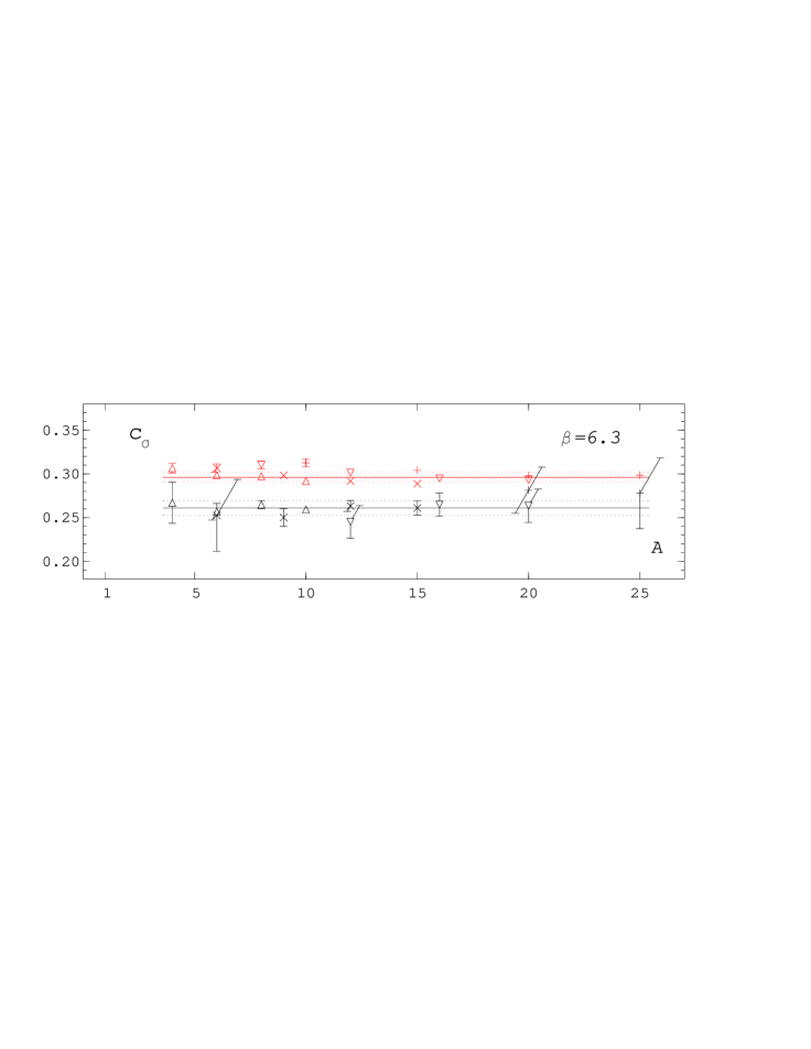
Figure 11: Comparison of the anisotropy coefficient $c_{\sigma}$ of the Wilson action from the matching of $R_{1}$ with $k\neq 1$ (black) and $k=1$ (red points) as a function of $A=m_{x}m_{y}$ for $\beta=6.3\,$. Points with $m_{x}=2,3,4,5$ are denoted by $\bigtriangleup,\times,\bigtriangledown,+\,$, respectively.

at $\beta=7.2$ the errors are larger because of the lower statistics of the measurements. The final results for $c_{\sigma}$ and $c_{\tau}$ are given in Table 2 . We obtained them by fitting the single values to a constant with the $\chi^{2}-$method. Their average errors were estimated from the error estimate of the constant times the square root of the number $N$ of fitpoints. The error estimate was rescaled whenever $\chi^{2}/(N-1)>2\,$. This was only necessary for $\beta=5.4\,$. In order to be able to compare our results to those of Klassen [18], we have repeated the matching analysis under the assumption $k=1\,$. Though the single matching results seem to have smaller errors then, a constant $\chi^{2}-$fit as before yields always a $\chi^{2}$ per degree of freedom which is larger than 2. The inclusion of small Wilson loops in the matching seems to be more crucial here and also to lead to higher values for $c_{\sigma}\,$. This is observed in Fig. 11, where we compare the two methods at $\beta=6.3\,$.

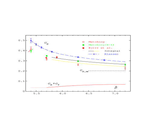
Figure 12: Comparison of all available data for the anisotropy coefficient $c_{\sigma}$ of the Wilson action. Further details are explained in the text.

Finally, we have gathered in Fig. 12 all available results for the Wilson action $c_{\sigma}\,$: those which we obtained from the integral method are represented by the fit, eq.(2.15), and the fit showing the possible influence of $p/T^{4}(\beta_{0})\,$; our matching results for $k\neq 1$ and $k=1\,$; the $SU(3)$ data of Ejiri et al.[15] and those of Klassen[18], both for our $\beta-$function. We observe consistent behaviour of the integral and matching results for $k=1\,$, those for $k\neq 1$ are still within the error bars (see Fig. 2). There is also full agreement with the data of Ejiri et al. . Only the results of Klassen are definitely higher and insofar incompatible with all other measurements of $c_{\sigma}\,$.

4 Anisotropy coefficients for improved actions

Up to now we have discussed in detail the calculation of the anisotropy coefficients for the Wilson action only. In the following we consider the more general family of actions defined by Wilson loops of size up to 4 in the ($\mu,\nu$)-plane

$$S_{\mu\nu}\!\!\!\! = \!\!\!\!a_{1,1}\left(1-\frac{1}{N_{c}}{\rm Re\,}{\rm Tr\,}\mbox{\raisebox{-1.13809pt}{\psfig{bbllx=211,bblly=332,bburx=360,bbury=481,height=11.38109pt}}~{}}\right)$$ (4.1)

$$\!\!\!\!+a_{1,2}\left(1-\frac{1}{2N_{c}}{\rm Re\,}{\rm Tr\,}\left(\mbox{\raisebox{-1.42262pt}{\psfig{bbllx=137,bblly=332,bburx=435,bbury=481,height=11.38109pt}}~{}}+\mbox{\raisebox{-7.68222pt}{\psfig{bbllx=211,bblly=258,bburx=360,bbury=556,height=22.76219pt}}~{}}\right)\right)+a_{2,2}\left(1-\frac{1}{N_{c}}{\rm Re\,}{\rm Tr\,}\mbox{\raisebox{-7.68222pt}{\psfig{bbllx=137,bblly=258,bburx=435,bbury=556,height=22.76219pt}}~{}}\right).$$

Here, the parameters $a_{11},~{}a_{12}$ and $a_{22}$ are constrained by the equation

$$a_{11}+4a_{12}+16a_{22}=1~{},$$ (4.2)

which ensures the correct continuum limit. The action is $O(a^{2})$ improved, if additionally

$$a_{12}={2\over 3}-{a_{11}\over 2}~{},\quad a_{22}={1\over 16}\left(a_{11}-{5\over 3}\right)~{}.$$ (4.3)

Still, one parameter, for example $a_{11}$, is free. For $a_{11}=5/3$ we obtain the Symanzik action ($a_{12}=-1/16,~{}a_{22}=0$), for $a_{11}=4/3$ the $(2\times 2)-$action ($a_{12}=0,~{}a_{22}=-1/48$). Alternatively, one may require that the propagator can be diagonalized. This facilitates the analytic calculation of the anisotropy coefficients in the weak coupling limit. In that case we have the condition

$$a_{11}={1\over(1+4z)^{2}}~{},\quad a_{12}=2za_{11}~{},\quad a_{22}=z^{2}a_{11}~{},$$ (4.4)

with the free parameter $z$. One can combine both objectives for a special set of parameters ($z=-1/16$)

$$a_{11}={16\over 9}~{},\quad a_{12}=-{2\over 9}~{},\quad a_{22}={1\over 144}~{}.$$ (4.5)

The corresponding action was introduced by García Pérez et al. [9] under the name Square Symanzik action. In ref. [19] the asymptotic $(\beta\rightarrow\infty)$ anisotropy coefficients of this action have actually been calculated. For $SU(3)$ one obtains

$$c_{\sigma}(0)=0.09829281~{},\quad c_{\tau}(0)=-0.03008298~{}.$$ (4.6)

It is therefore obvious to investigate the properties of this action further and in particular to determine its anisotropy coefficients non-perturbatively. For comparison we have as well considered the somewhat simpler $(2\times 2)-$action, which is improved, but its perturbative anisotropy coefficients are unknown.

In order to apply the integral method we need again the high temperature limits of energy density and pressure. For the Square Symanzik action we have derived the expansions corresponding to eqs. (2.9) and (2.10)

$$\!\!R_{D}(N_{\tau})\!\!\! = \!\!\!1-{40\over 231}\left({\pi\over N_{\tau}}\right)^{6}-{176896\over 3869775}\left({\pi\over N_{\tau}}\right)^{8}+O\left(N_{\tau}^{-10}\right)$$

$$\approx \!\!\!1-0.1732\left({\pi\over N_{\tau}}\right)^{6}-0.0457\left({\pi\over N_{\tau}}\right)^{8}+O\left(N_{\tau}^{-10}\right)~{};$$

$$\!\!R_{I}(N_{\tau})\!\!\! = \!\!\!1-{8\over 105}\left({\pi\over N_{\tau}}\right)^{4}-{80\over 693}\left({\pi\over N_{\tau}}\right)^{6}-{420128\over 4729725}\left({\pi\over N_{\tau}}\right)^{8}+O\left(N_{\tau}^{-10}\right)$$

$$\approx \!\!\!1-0.076\left({\pi\over N_{\tau}}\right)^{4}-0.115\left({\pi\over N_{\tau}}\right)^{6}-0.089\left({\pi\over N_{\tau}}\right)^{8}+O\left(N_{\tau}^{-10}\right)~{}.$$

By chance, the ratio $R_{D}(N_{\tau})$ is even $O(a^{4})$ improved. Since we intend to make use of Monte Carlo simulations on $N_{\tau}=4$ lattices we list in Table 3 the respective numerical results for the complete $1/N_{\tau}-$expansions of the ratios. The numbers for the $(2\times 2)-$action have been taken from ref. [12].

Action	$R_{D}$	$R_{I}$	$r=R_{D}/R_{I}$
$(2\times 2)$	1.088	0.99	1.099
Square Sym.	0.957	0.91	1.052

Table 3: Derivative ($R_{D}$) and integral method ($R_{I}$) ratios at $N_{\tau}=4$ for the $(2\times 2)$ and the Square Symanzik actions.

4.1 Results for the ${\bf(2\times 2)-}$action

The thermodynamics of the $SU(3)~{}(2\times 2)-$action has already been investigated in detail by simulations on $24^{3}\times 4$ and $24^{4}$ lattices in ref. [12]. We can therefore immediately apply the integral method to compute the anisotropy coefficients using the corresponding plaquette expectation values and the $\beta-$function. For $N_{\tau}$=4 the critical coupling was found to be $\beta_{c}=4.3995(2)\,$. The behaviour of $c_{\sigma}$ is similar to that shown in Fig. 2 for the Wilson action. With increasing $\beta$ $c_{\sigma}$ is slowly decreasing. In the neighbourhood of the critical point the integral method leads again to numerical difficulties.

$\beta$	4.4	5.0	5.9
$c_{\sigma}$	0.226(08)	0.157(16)	0.115(16)
$c_{\tau}$	-0.190(08)	-0.096(16)	-0.067(16)
$c_{\sigma}(k=1)$	0.236(03)	0.195(07)	0.158(13)
$c_{\tau}(k=1)$	-0.200(03)	-0.134(07)	-0.110(13)

Table 4: The matching results for $c_{\sigma}$ and $c_{\tau}$ for the $(2\times 2)-$action.

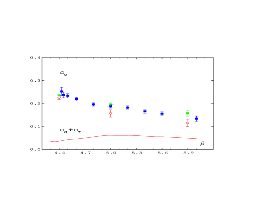
Figure 13: The anisotropy coefficient $c_{\sigma}$ of the $(2\times 2)-$action from the integral (blue squares) and matching methods (circles). Results from fixed $k=1$ matching fits are shown as green squares.

In Fig. 13 we compare the integral method results with matching results, which were obtained on anisotropic $24^{4}$ lattices with 2000-4000 Wilson loop measurements for $\beta=4.4$ and 5.0 and 600 for $\beta=5.9\,$. We note, that due to the inclusion of $(2\times 2)-$Wilson loops in the action, less links can be integrated to increase the accuracy of the measurements. In Table 4 we present the values for $c_{\sigma}$ and $c_{\tau}$ from the matching procedure. Again we observe, that the matching with fixed $k=1$ leads to somewhat higher values. We find agreement between the different methods, but like for the case of the Wilson action only after taking into account the cut-off correction factor $r$ from Table 3.

4.2 Results for the Square Symanzik action

In order to determine the $\beta-$function for this action we have performed simulations on $24^{4}$ lattices and measured the plaquettes and the string tension as in ref. [20]. The lattice result $\hat{\sigma}(\beta)$ and the physical string tension $\sigma$ are related by $\hat{\sigma}(\beta)=\sigma a^{2}\,$. The $\beta-$function is then derived from

$$a{dg^{-2}\over da}={a\over 2N_{c}}{d\beta\over da}={\sqrt{\hat{\sigma}}\over 2N_{c}}\left({d\sqrt{\hat{\sigma}(\beta)}\over d\beta}\right)^{-1}~{}.$$ (4.9)

In Fig. 14 we show our measured values for $\sqrt{\hat{\sigma}(\beta)}$ together with a fit from which we have deduced the numerical values of the $\beta-$function. On a $24^{3}\times 4$ lattice we have then measured the generalized plaquettes $P_{\sigma}$ and $P_{\tau}$ as well as the Polyakov loop and its susceptibility in the range $3.9\leq\beta\leq 6.0\,$. On the average we took 4000-8000, close to the critical point 18000 measurements. From the peak of the susceptibility we estimate the following critical coupling for $N_{\tau}=4$

$$\beta_{c}=3.9820\,(\begin{array}[c]{c}\scriptstyle+8\\ \scriptstyle-5\end{array})~{}.$$ (4.12)

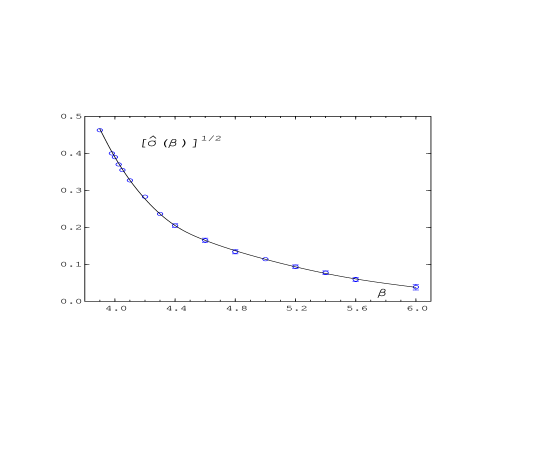
Figure 14: The square root of the string tension, $\sqrt{\hat{\sigma}(\beta)}$ for the $SU(3)$ Square Symanzik action. The line is a fit to the data.

As a side product of our calculations we obtain the ratio

$${T_{c}\over\sqrt{\sigma}}={1\over N_{\tau}\sqrt{\hat{\sigma}(\beta_{c})}}=0.643(4)~{},$$ (4.13)

which is in agreement with results found for other improved actions [21]. Using the above mentioned data and $r$ from Table 3 we have again applied the integral method to find the anisotropy coefficient $c_{\sigma}\,$. It is shown in Fig. 15 together with the asymptotic value $c_{\sigma,\infty}\,$, eq. (4.6), and the results of our matching analysis. The latter are also listed in Table 5. They were obtained from Wilson loop measurements on $24^{4}$ lattices. Like for the $(2\times 2)-$action less link integrations than in the Wilson action case can be done. Comparing the different results in Fig. 15 we find again the same general $\beta-$dependence as for the other actions. Also, a sizeable difference between the different matching options for $k$ is found: the $k=1$ results show an even stronger influence of the Wilson loop area as before, the $k\neq 1$ results agree nicely with the integral method data. We note that $c_{\sigma}$ in the Square Symanzik case is about half as big as in the Wilson case.

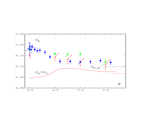
Figure 15: The anisotropy coefficient $c_{\sigma}$ of the Square Symanzik action from the integral (blue squares) and matching methods (circles). Results from fixed $k=1$ matching fits are shown as green squares. The dashed black line shows $c_{\sigma,\infty}\,$.

$\beta$	4.0	4.5	4.75	5.0	5.5
$N_{meas}$	2000	800-1000	700	500-1500	200
$c_{\sigma}$	0.149(11)	0.143(17)	0.132(20)	0.119(18)	0.109(21)
$c_{\tau}$	-0.102(11)	-0.065(17)	-0.042(20)	-0.031(18)	-0.033(21)
$c_{\sigma}(k=1)$	0.175(03)	0.158(06)	0.155(09)	0.157(09)	0.120(13)
$c_{\tau}(k=1)$	-0.128(03)	-0.080(06)	-0.065(09)	-0.069(09)	-0.044(13)

Table 5: The matching results for $c_{\sigma}$ and $c_{\tau}$ for the Square Symanzik action. $N_{meas}$ is the number of Wilson loop measurements .

5 Summary and conclusions

One of the major objectives of our paper was the verification of the equivalence of the integral and derivative methods for the calculation of thermodynamic quantities like energy density and pressure. The major obstacle in the comparison of the methods is the cut-off dependence on finite lattices. In the high temperature limit the deviations of energy density and pressure from their respective continuum limits due to the cut-off effects can be calculated. They manifest themselves as a dependence on $1/N_{\tau}^{2}$ in the thermodynamic limit, and they are different for the two methods.

The anisotropy coefficients as such must be finite size independent. Their calculation allows then for a check on the internal consistency of the integral method and of its equivalence to the derivative method. Moreover, its non-perturbative behaviour is of importance for the approach of thermodynamic quantities to the continuum limit.

By taking into account the major cut-off effects through the correction factor $r$ we have shown for the Wilson action that one obtains similar results for $N_{\tau}$=4, 6 and 8 which agree, inside error bars, also with the matching results and with the results of Ejiri et al.[15]. The $c_{\sigma}-$data of Klassen[18] are however definitely higher. This may be connected to the difference in our matching methods, the accuracy of the data and the lattice sizes used. We found it essential for the application of the matching procedure, that link integration of the Wilson loops was carried out, wherever this was possible, and that ratios instead of Wilson loops directly were used for the matching. Thus we avoided perimeter and corner dependencies. Remaining effects of this kind are probably responsible for the difference of $k=1$ to $k\neq 1$ matching fits. The fact that $\xi(\gamma)$ was linear near $\gamma=1$ helped in the determination of the derivative $(\partial\xi/\partial\gamma)_{\xi=1}$.

We have repeated our analysis for two improved actions, the $(2\times 2)$ and the Square Symanzik action, and find similar behaviours of the corresponding anisotropy coefficients. For all investigated actions the non-perturbative $c_{\sigma}$ decrease with increasing $\beta$ and approach their respective weak coupling limits from above; the results from the matching and integral methods are in all cases compatible with each other.

In addition we determined for the Square Symanzik action the deconfinement transition point $\beta_{c}$ for $N_{\tau}=4\,$, the ratio $T_{c}/\sqrt{\sigma}$ and the $\beta-$function in terms of the string tension. As an analytic result we derived the thermodynamic high temperature limits for this action.

Acknowledgements

We thank Maria García Pérez for providing us with details of her work in refs. [9] and [19]. The help of Burkhard Sturm (alias B. Beinlich) in the calculation of the determinant of the inverse propagator and the high temperature limits is gratefully acknowledged. The work was partly supported by the Deutsche Forschungsgemeinschaft under grants Pe 340/3-3 and Ka 1198/4-1, and the European Commission under the TMR-Network ”Finite Temperature Phase Transitions in Particle Physics”, ERBFMRX-CT-97-0122.

References

- [1] G. Burgers, F. Karsch, A. Nakamura and I.O. Stamatescu, Nucl. Phys. B 304 (1988) 587.
- [2] J. Engels, F. Karsch, I. Montvay and H. Satz, Nucl. Phys. B 205[FS5] (1982) 545.
- [3] F. Karsch, Nucl. Phys. B 205 (1982) 285.
- [4] B. Svetitsky and F. Fucito, Phys. Lett. 131 B (1983) 165.
- [5] Y. Deng, Nucl. Phys. B (Proc. Suppl.) 9 (1989) 334; F.R. Brown, N.H. Christ, Y. Deng, M. Gao and T. Woch, Phys. Rev. Lett. 61 (1988) 2058.
- [6] J. Engels, J. Fingberg, F. Karsch, D. Miller and M. Weber, Phys. Lett. 252 B (1990) 625.
- [7] G. Boyd, J. Engels, F. Karsch, E. Laermann, C. Legeland, M. Lütgemeier and B. Petersson, Nucl. Phys. B 469 (1996) 419.
- [8] J. Engels, F. Karsch and T. Scheideler, Nucl. Phys. B (Proc. Suppl.) 63A-C (1998) 427.
- [9] M. García Pérez, J. Snippe and P. van Baal, 2nd Workshop on Continuous Advances in QCD, Minneapolis, March 1996, hep-lat/9607007.
- [10] K. Akemi et al. (QCDTARO Collaboration), Phys. Rev. Lett. 71 (1993) 3063.
- [11] R.G. Edwards, U.M. Heller and T.R. Klassen, Nucl. Phys. B 517 (1998) 377.
- [12] B. Beinlich, F. Karsch and E. Laermann, Nucl. Phys. B 462 (1996) 415.
- [13] J. Engels and T. Scheideler, Nucl. Phys. B 539 (1999) 557.
- [14] J. Engels, F. Karsch and K. Redlich, Nucl. Phys. B 435 (1995) 295.
- [15] S. Ejiri, Y. Iwasaki and K. Kanaya, Phys. Rev. D 58 (1998) 094505.
- [16] J.D. Stack, Phys. Rev. D 27 (1983) 412.
- [17] Ph. de Forcrand and C. Roiesnel, Phys. Lett. 151 B (1985) 77.
- [18] T.R. Klassen, Nucl. Phys. B 533 (1998) 557.
- [19] M. García Pérez and P. van Baal, Phys. Lett. B 392 (1997) 163.
- [20] B. Beinlich, C. Legeland, M. Lütgemeier, A. Peikert and T. Scheideler, Nucl. Phys. B (Proc. Suppl.) 63A-C (1998) 260.
- [21] B. Beinlich, F. Karsch, E. Laermann, and A. Peikert, Eur. Phys. J. C 6 (1999) 133.