PITHA 99/13
Mass spectrum and elastic scattering in the massive $SU(2)_{f}$ Schwinger model on the lattice

Abstract

We calculate numerically scattering phases for elastic meson–meson scattering processes in the strongly coupled massive Schwinger–model with an SU(2) flavour symmetry. These calculations are based on Lüscher’s method in which finite size effects in two–particle energies are exploited. The results from Monte–Carlo simulations with staggered fermions for the lightest meson (“pion”) are in good agreement with the analytical strong–coupling prediction. Furthermore, the mass spectrum of low–lying mesonic states is investigated numerically. We find a surprisingly rich spectrum in the mass region $[m_{\pi},4m_{\pi}]$.

PACS: 11.10.Kk, 11.15.Ha
Keywords: Lattice gauge theory; Schwinger model; mass spectrum; elastic scattering phases

1 Introduction

Present experiments at high energy accelerators are mainly scattering experiments. A task for theoretical QCD is to calculate quantities which can be compared to the data of such scattering experiments. In deep inelastic scattering processes for example, reliable results are obtained by perturbative calculations. But problems occur in experiments with small momentum transfers. These are, e.g., resonant elastic scattering processes, like the occurrence of the $\rho$–resonance and the $\Delta$–resonance in $\pi$–$\pi$ and $\pi$–$p$ respectively scattering processes. For such low–energy phenomena perturbative calculations in the strongly–coupled QCD region are not suitable.

By contrast there exists an appropriate method in the framework of lattice calculations proposed by Lüscher in which scattering phases of the continuum theory can be calculated for elastic scattering processes in massive quantum field theories [1, 2, 3]. In this method one makes use of the fact that for large but finite spatial extension the volume dependence of the energies of two–particle states is determined by the S–matrix for elastic scattering processes in infinite volume. As the determination of energies in finite volumes is possible in Monte–Carlo simulations this method is very useful for lattice calculations.

There are many successful applications of this method for the calculation of scattering phases in bosonic models in two and four dimensions [4, 5, 6, 7, 8, 9, 10]. The basic formulae for Lüscher’s method have also been derived in a fermionic theory [11]. The agreement of the numerical data with the predicted scattering phases for the fermion–fermion scattering in the Gross–Neveu model in two dimensions [12] confirms the usefulness of Lüscher’s method also in fermionic models.

Our aim is the application of Lüscher’s method to the determination of elastic scattering phases in a meson–meson system of the massive Schwinger model with an ${\mbox{SU(2)}}_{f}$ flavour symmetry in the continuum. The experience gained in this project shall support future investigations in the QCD, e.g. of the $\rho$–resonance in the $\pi^{+}\pi^{-}\rightarrow\rho^{0}\rightarrow\pi^{+}\pi^{-}$ scattering process. In this context the Schwinger model has some useful features: The Schwinger model is a fermionic gauge field theory which has many properties in common with QCD, such as confinement, the $U(1)_{A}$ anomaly and a non–trivial vacuum structure. In particular the massive Schwinger model with $N_{f}=2$ offers a complex mass spectrum and therefore conditions (and problems) comparable to QCD with $u$,$d$–quarks as far as the mesonic energy spectrum is concerned. Furthermore, the simulations for the determination of the scattering phases are extensive, e.g. because of the calculation of fermionic eight–point functions. Therefore a two–dimensional model has the advantage to be not as expensive to simulate as the four–dimensional QCD.

Another advantage of the massive Schwinger model with $N_{f}=2$ is that there exist analytical predictions for strong couplings: The massive ${\mbox{SU(2)}}_{f}$ Schwinger model is not analytically solved. But for strong coupling the “pion sector” of this model, i.e. the sector in which the lightest meson–triplet (“pions”) occurs, can be approximated by the sine–Gordon model. In the sine–Gordon model the mass spectrum and the elastic S–matrix have been calculated [13, 14, 15]. The primary aim of our investigations is the comparison of the predictions for the scattering phases from the sine–Gordon model with the numerical results in the massive ${\mbox{SU(2)}}_{f}$ Schwinger model calculated with the procedure of Lüscher. By this comparison we also check ambiguities, the CDD–poles [15], in the analytical result for the S–matrix.

For a successful determination of the scattering phases it is necessary to have a good knowledge of the mass spectrum in the massive ${\mbox{SU(2)}}_{f}$ Schwinger model:

First, investigating the particle masses in the pion sector we determine the strong coupling region in which the approximation of the pion sector by the sine–Gordon model and thus the prediction for the scattering phases of the pion–pion scattering are nearly exact. Secondly, the analysis of the mass spectrum is useful to estimate the energies of possible additional scattering processes besides the $\pi$–$\pi$ scattering and of inelastic thresholds in the energy region of the elastic $\pi$–$\pi$ scattering. Thirdly, we investigate systematically lattice artifacts — finite size and ${{\cal O}(a)}$ effects — affecting the particle masses. Such investigations are very important because small systematical deviations in the two–particle energies lead to large errors in the scattering phases calculated from these energies.

The paper is organized as follows: In section 2 the known analytical results for the mass spectrum and the scattering phases are summarized. In section 3 the numerical methods, especially an improved method for the determination of energies from correlation matrices, are discussed. The relation of the symmetry groups on the lattice and in the continuum is described in section 4. In section 5 the numerical results for the mass spectrum of the massive ${\mbox{SU(2)}}_{f}$ Schwinger model are presented. The numerical results for the scattering phases for the elastic $\pi$–$\pi$ scattering are compared to the analytical prediction in section 6. In this section also the contributions of single–particle states and of states of two non–interacting pions to four–meson correlation functions are discussed. The paper ends with a summary of the main results.

2 Analytical predictions in the massive ${\mbox{SU(2)}}_{f}$ Schwinger model

2.1 Bosonization

In Minkowskian space–time the action of the massive Schwinger model with a ${\mbox{SU(2)}}_{f}$ flavour symmetry is:

$$S = \int d^{2}x\left\{-\frac{1}{4}F_{\mu\nu}F^{\mu\nu}+\sum_{f=1,2}{\bar{\psi}}^{f}(i\partial\!\!\!/-eA\!\!\!/-m_{0})\psi^{f}\right\},$$

$$\hskip 28.45274ptF_{\mu\nu}=\partial_{\mu}A_{\nu}-\partial_{\nu}A_{\mu}\,,\hskip 14.22636pt\left\{\gamma_{\mu},\gamma_{\nu}\right\}=2g_{\mu\nu}\hskip 4.30554pt.$$

This model has many properties in common with the four–dimensional QCD: In the massless case ($m_{0}=0$) there exists an anomalous axial $U(1)$–current [16] and a massive meson (“$\eta$”–meson) which corresponds to the $\eta^{\prime}$–meson in QCD. Also the vacuum structure of the Schwinger model is not trivial. Analogously to the screening of colour charges of test particles in QCD with dynamical quarks the electric charge of test particles in the Schwinger model is completely screened. Furthermore, the “quarks” which denote the fundamental fermions in (2.1) are confined in the massive Schwinger model with $N_{f}=2$ for $|\Theta|\neq\pi/2$. Thus there exist no free states with a non–zero fermion number [17].

The basis for the bosonization of the Schwinger model is the equivalence between the sine–Gordon model and the massive Thirring–model [18]. This equivalence gives the possibility to express the fermionic fields $\psi^{1}$, $\psi^{2}$ (and also the gauge fields by means of the equation of motion) in (2.1) by two bosonic fields $\phi_{+}$ and $\phi_{-}$. The bosonized form of (2.1) which is obtained this way was derived in ref. [19]. In Hamiltonian formulation one obtains:

$${\mathscr{H}} = :\frac{1}{2}\Pi^{2}_{+}+\frac{1}{2}(\partial_{1}\phi_{+})^{2}+\frac{\mu^{2}}{2}\phi^{2}_{+}:_{\mu}\>+:\frac{1}{2}\Pi^{2}_{-}+\frac{1}{2}(\partial_{1}\phi_{-})^{2}:_{m_{0}}$$ (2)

$$-2cm_{0}^{3/2}\mu^{1/2}:\cos\left(\sqrt{2\pi}\phi_{+}\right):_{\mu}\>:\cos\left(\sqrt{2\pi}\phi_{-}\right):_{m_{0}}\hskip 4.30554pt.$$

$:\,\,\,:_{\mu,m_{0}}$ denotes normal ordering with respect to a free field with mass $\mu$ and $m_{0}$ respectively. $\Pi_{+}$ and $\Pi_{-}$ are the conjugate momenta of the Bose fields $\phi_{+}$ and $\phi_{-}$. The parameter $\mu$ is defined as $\mu\equiv e\sqrt{2/\pi}$. The constant $c$ stems from the bosonization formulae of the massive Thirring model and has the value $c=\exp(\gamma)/(2\pi)$ [20] ($\gamma$ is the Euler constant).

We now confine ourselves to the strong coupling limit of the model, i.e. to the case where $m_{0}/e\ll 1$. Expanding the cosine–terms in (2) the mass scale of the $\phi_{-}$– and $\phi_{+}$–fields is given by $(m_{0}^{3/2}\mu^{1/2})^{1/2}$ and $\mu$ respectively. For $m_{0}/\mu\ll 1$ the $\phi_{+}$–field has a much higher mass in (2) than the $\phi_{-}$–field. Hence for $m_{0}/e$ small the $\phi_{+}$–field has only small effects on the dynamics of the $\phi_{-}$–fields so that the $\phi_{+}$–$\phi_{-}$ interaction terms in (2) are negligible if only the $\phi_{-}$–field is considered. With these approximations one finally obtains with small $m_{0}/e$ the following theory for the $\phi_{-}$–field [19]:

$${\mathscr{H}_{\phi_{-}}} = :\frac{1}{2}\Pi^{2}_{-}+\frac{1}{2}(\partial_{1}\phi_{-})^{2}-\frac{m^{\prime 2}}{\beta_{SG}^{2}}\cos(\beta_{SG}\,\phi_{-}):_{m^{\prime}}\,,$$

$$\hskip 28.45274ptm^{\prime}=2\sqrt{2\pi}c^{2/3}\left(\frac{m_{0}}{e}\right)^{2/3}e\,,\hskip 14.22636pt\beta_{SG}=\sqrt{2\pi}\hskip 4.30554pt.$$

This Hamiltonian represents the sine–Gordon model with a coupling parameter $\beta_{SG}$. Hence it is possible to make use of the analytical results for the sine–Gordon model in order to obtain predictions for the lightest particles in the Schwinger model. The approximation of the Schwinger model by the sine–Gordon model is, of course, only valid in the $\phi_{-}$–sector (“pion sector”) of the Schwinger model for $m_{0}/e$ small.

2.2 Mass spectrum and scattering phases

The sine–Gordon model is an integrable model. Solutions for the mass spectrum in the quantized theory have been first derived in a semi–classical approximation [13]. The mass of the soliton ($A$) and antisoliton ($\bar{A}$) is predicted to be

$$M_{A}=M_{\bar{A}}=\frac{8m^{\prime}}{\gamma^{\prime}},\hskip 28.45274pt\frac{1}{\gamma^{\prime}}\,{:=}\,\frac{1}{\beta_{SG}^{2}}-\frac{1}{8\pi}\hskip 4.30554pt.$$ (4)

The number of additional stable particles $B_{n}$, $n=1,2\ldots<8\pi/\gamma^{\prime}$ depends on the parameter $\beta_{SG}$. In the case $\beta_{SG}=\sqrt{2\pi}$ there exist two stable states $B_{1}$ and $B_{2}$ with masses $M_{1}=M_{A}$ and $M_{2}=\sqrt{3}\,M_{A}$. Hence for $m_{0}/e\rightarrow 0$ there are four particles in the Schwinger–model which are related to the $\phi_{-}$–sector. The ${\mbox{SU(2)}}_{f}$ flavour symmetry of the Schwinger model is visible in the sine–Gordon model for $\beta_{SG}=\sqrt{2\pi}$ as the particle spectrum consists of a triplet ($A$,$\bar{A}$,$B_{1}$) and a singlet ($B_{2}$). The quantum numbers ($I$sospin, $P$arity, $G$–parity) of the triplet are $I^{PG}=1^{-+}$ and of the singlet $I^{PG}=0^{++}$ [19]. In analogy to QCD we call the pseudoscalar triplet “pion” and the $0^{++}$–particle “$f_{0}$”–meson. From (2.1) and (4) one obtains for the pion mass in the Schwinger model

$$m_{\pi} = 6\sqrt{\frac{2}{\pi}}c^{2/3}\left(\frac{m_{0}}{e}\right)^{2/3}e$$ (5)

$$\simeq 2.066\left(\frac{m_{0}}{e}\right)^{2/3}e$$

and for the $f_{0}$–mass

$$m_{f_{0}} = \sqrt{3}\,m_{\pi}\hskip 4.30554pt.$$ (6)

Exact calculations for the mass gap in the sine–Gordon model in the full quantum field theory show that the semiclassical results are nearly exact [14, 21]. The difference of the exact result

$$m_{\pi} \simeq 2.008\left(\frac{m_{0}}{e}\right)^{2/3}e$$ (7)

for the pion mass to the semiclassical formula (5) is about $3\%$.

In the original derivation of the Hamiltonian (2.1) in ref. [19] the parameter $m^{\prime}$ contains the additional factor $(\cos(\Theta/2))^{2/3}$ with $\Theta\in[-\pi,\pi]$. This factor reduces the pion mass in (5) and (7) for $\Theta\neq 0$. All our Monte–Carlo simulations yield numerical data for the pion mass which are above the values of (5), indicating $\Theta\simeq 0$. Therefore we put $\Theta=0$ in all relevant formulae in this paper.

Besides the particles which have their origin in the $\phi_{-}$–sector there exists a particle in the Schwinger model resulting from the $\phi_{+}$–field in (2). It has quantum numbers $I^{PG}=0^{--}$ (“$\eta$”–meson) [19]. In the massless limit $m_{0}\rightarrow 0$ it becomes the massive boson of the massless model with mass [17]

$$m=\mu\equiv e\sqrt{\frac{2}{\pi}}\hskip 4.30554pt.$$ (8)

In the massive theory we therefore expect for $m_{0}/e\ll 1$ a mass of the order $m_{\eta}\simeq\mu$. Other states whose mass is above the mass of the $\pi$–, $f_{0}$– and $\eta$–meson can exist because of the $\phi_{+}$–$\phi_{-}$ interaction and the $\phi_{+}$ self–interactions in (2). Many of such possibly unstable states have been found in our numerical simulations (see section 5.4).

To obtain an analytical formula for the elastic scattering phases for the pion–pion scattering in the strongly coupled Schwinger model one can once again make use of its approximation by the sine–Gordon model. The S–matrix in the sine–Gordon model has been derived exactly [15]. The calculation is based on the unitarity and crossing–symmetry as well as on the factorization property of the S–matrix in the sine–Gordon model. For $\beta_{SG}=\sqrt{2\pi}$ one obtains the same scattering matrix element $S(\theta)$ for the three possible scattering processes with soliton ($A$) and antisoliton ($\bar{A}$): $AA\longrightarrow AA$, $A\bar{A}\longrightarrow A\bar{A}$, $\bar{A}\bar{A}\longrightarrow\bar{A}\bar{A}\,$:

$$S(\theta)=\frac{\sinh(\theta)+i\sin{\pi/3}}{\sinh(\theta)-i\sin{\pi/3}}\hskip 4.30554pt.$$ (9)

The difference of the rapidities $\theta_{1}$ and $\theta_{2}$ of the two particles is denoted by $\theta$: $\theta=\theta_{1}-\theta_{2}$. It is related to the particle momentum $k$ by $\theta=2\,\mbox{arsinh}(k/M_{A})$. Equation (9) is an approximation for the scattering matrix element for the elastic pion–pion scattering in the strongly coupled Schwinger model. Defining scattering phases $\delta(\theta)$ via

$$S(\theta) \equiv {e^{2i\delta(\theta)}}$$ (10)

one obtains the connection $\delta(k/m_{\pi})$ between the elastic scattering phases and the particle momenta. The aim of our numerical investigations is to compare the scattering phases $\delta(k/m_{\pi})$ obtained by the method of Lüscher with Monte–Carlo simulations with the analytical results (9).

The scattering matrix element (9) is unique up to multiplicative “CDD”–terms:

$$f(\theta)=\prod_{k=1}^{L}\frac{\sinh(\theta)+i\sin(\alpha_{k})}{\sinh(\theta)-i\sin(\alpha_{k})}\,,\hskip 28.45274pt\alpha_{k}\in\mathbb{R}\hskip 4.30554pt.$$ (11)

Expression (9) is the “minimal” solution with the lowest number of poles. Arguments that this minimal solution for the soliton–soliton scattering in the sine–Gordon model is exact were given in ref. [15]: There exist two states in the sine–Gordon model for $\beta_{SG}=\sqrt{2\pi}$ with masses $M_{A}$ and $\sqrt{3}M_{A}$ which can be interpreted as bound states of soliton and antisoliton. This corresponds to the two poles $\theta=i\pi/3$ and $\theta=i2\pi/3$ in the scattering matrix element (9) of the soliton–antisoliton scattering. Furthermore, the minimal solution is in agreement with the results for the S–matrix in the semiclassical limit $\beta_{SG}\rightarrow 0$. Our numerical results discussed in section 6.5 also support the scattering phases of the minimal solution.

Because of the factorization property of the S–matrix the scattering matrix elements of scattering processes involving the states $B_{n}$ can be calculated by using the scattering matrix element of the soliton–soliton scattering. The states $B_{n}$ can be interpreted as bound states of soliton and antisoliton. Hence arbitrary scattering processes can be understood as a sequence of scattering processes between soliton and antisoliton. Calculating for $\beta_{SG}=\sqrt{2\pi}$ the scattering matrix elements for the processes $B_{1}A\rightarrow B_{1}A$, $B_{1}\bar{A}\rightarrow B_{1}\bar{A}$ and $B_{1}B_{1}\rightarrow B_{1}B_{1}$ one obtains in each case the expression (9). Hence all scattering processes within the triplet ($A$, $\bar{A}$, $B_{1}$) have the same scattering matrix element. That means that the elastic scattering phases for the $\pi$–$\pi$–scattering in the Schwinger model for $m_{0}/e\rightarrow 0$ are identical for all isospin channels.

3 Numerical methods

Our starting point for Monte–Carlo simulations of the Schwinger model is its Euclidean lattice action with Kogut–Susskind fermions:

$$S = S_{W}+\sum_{x,y}{\bar{\chi}_{x}}{M(x,y)}{\chi_{y}}\,,$$ (12)

$$S_{W} = \beta\sum_{x}\left\{1-\mbox{Re}\,U_{p}(x)\right\}\,,$$

$$\hskip 14.22636pt\hskip 14.22636ptU_{p}(x)\,{:=}\,U^{\ast}_{2}(x)U^{\ast}_{1}(x+\hat{2})U_{2}(x+\hat{1})U_{1}(x)\,,$$

$${M(x,y)} = \frac{a}{2}\sum_{\mu}\eta_{\mu}(x)\left\{{U(x,x+\hat{\mu})}\delta_{x+\hat{\mu},y}-{U(x,x-\hat{\mu})}\delta_{x-\hat{\mu},y}\right\}$$ (13)

$$+m_{0}a^{2}\delta_{x,y}\,,\hskip 14.22636pt\hskip 14.22636pt\eta_{1}(x)=1\,,\,\,\eta_{2}(x)=(-1)^{x_{1}}\hskip 4.30554pt.$$

The sum over the space–time coordinates $x=(x_{1},x_{2})$ runs for the space coordinate $x_{1}\equiv{\bf{x}}$ from $a$ to $La$ and for the time coordinate $x_{2}\equiv t$ from $a$ to $Ta$. We use the Wilson action with the link variables $U_{\mu}(x)$ as a compact formulation of the gauge fields: $U_{\mu}(x)\equiv U(x+\hat{\mu},x)\in U(1)$. The Kogut–Susskind fermions ${\bar{\chi}},\chi$ on the lattice have one flavour so that a two–flavour Schwinger model in the continuum is simulated. In the simulations we use periodic boundary conditions for the link variables and periodic boundary conditions in space and antiperiodic in time for the fermionic fields.

In the naive continuum limit the parameter $\beta$ has to be chosen $\beta=1/(e^{2}a^{2})$ to obtain the continuum action of the Schwinger model. Therefore for finite $a$ we define a coupling $e$ on the lattice by $e\,{:=}\,\beta^{-1/2}$. Here and in the following the lattice constant $a$ is set to one. Dimensional and dimensionless parameters and fields are denoted by the same symbols provided there is no confusion.

3.1 HMC and topological ergodicity

We use the Hybrid Monte Carlo (HMC) method with pseudofermions and the conjugate gradient algorithm for the inversion of the fermion matrix. The HMC provides an efficient algorithm for the calculation of Euclidean path integrals in the Schwinger model. For $\beta\leq 5$ it appears to be ergodic with respect to the transition between different topological sectors (“topological ergodicity”). Topological sectors are characterized by the topological charge $Q$ of the gauge field configurations. We use the geometrical definition of refs. [22, 23]:

$$Q=\frac{1}{2\pi}\sum_{x}\theta_{p}(x)\hskip 4.30554pt.$$ (14)

$\theta_{p}\in(-\pi,\pi]$ is the plaquette angle which is defined by $U_{p}(x)=\exp(i\theta_{p})$. The tunneling probability $p_{T}$, i.e. the probability for a change of the topological sector in the HMC simulations, is about $10\%$ for $\beta=5$ and for ten trajectories between the measurements, reaching an acceptance probability of about 60-70%. The probability distribution of the topological charge $p(Q)$ for this coupling is plotted in fig. 1.

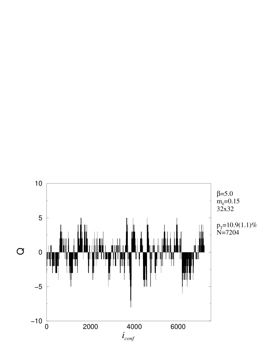
Figure 1: Probability distribution and time series of the topological charge $Q$ for a typical simulation with $N=7204$ configurations for ($\beta=5$, $m_{0}=0.15$).

Its shape can be understood phenomenologically from investigations in the pure $U(1)$ theory [24]. The mean action (and also the minimum action) in each topological sector is proportional to $Q^{2}$ on large lattices. Assuming a Boltzmann distribution one obtains a Gaussian like shape for $p(Q)$ as in fig. 1. The difference of the mean (and minimum) value of the action for adjacent topological sectors increases for increasing $\beta$. Therefore the width of $p(Q)$ becomes smaller for larger $\beta$ values so that for $\beta\geq 10$ almost only the sector $Q=0$ contributes.

In the quasi microcanonical calculation of the trajectories in the Hybrid Monte Carlo the action serves as a potential. Hence one is confronted with the problem that for high $\beta$–values the tunneling between adjacent topological sectors is suppressed. In fact the tunneling probability $p_{T}$ for $\beta\geq 10$ is far below $0.1\%$. In that case the HMC algorithm is not suitable to perform simulations having topological ergodicity, which is also known from QCD. This is, however, only a practical problem for the calculation of ensembles of moderate size which becomes less relevant on very large ensembles.

Another problem follows from the fact that the correlation functions have different values in different topological sectors: In contrast to investigations for $\beta=1$ [25] it turns out that for high values of $\beta$ the pion mass differs significantly for different topological sectors [26]. Also the exponential decay of the correlation function $C(t)$ for the pion is modified for $Q\neq 0$ (see ref. [27] for Wilson–fermions). For large $t$ and $|Q|$ the values of $C(t)$ are substantially smaller than it is expected for a pure exponential decay. Thus it is only possible for small values of $t$ and $|Q|$ to determine the pion mass by fits with exponential functions. But one is interested in high $\beta$–values as the continuum limit $a\rightarrow 0$ of the Schwinger model requires $\beta\rightarrow\infty$. A possible solution to the problems is the introduction of improved HMC algorithms which force the tunneling between different topological sectors [28, 29].

We have chosen an alternative way by calculating expectation values for $\beta\geq 10$ only for $Q=0$. We started the Monte–Carlo simulations with a suitable gauge configuration with $Q=0$. Because of the small $p_{T}$ for $\beta\geq 10$ the generation of ensembles of ${{\cal O}(50000)}$ was possible without tunneling into sectors $Q\neq 0$. This procedure is justified because the probability distribution $p(Q)$ of the topological charge for $\beta\geq 10$ is quite narrow. Hence the expectation value of an operator $O$ which can be decomposed on the lattice as

$$\left\langle\,O\,\right\rangle=\sum_{\nu=-\infty}^{\infty}\left\langle\,O\,\delta_{Q[U],\nu}\,\right\rangle$$ (15)

is dominated by the $Q=0$ sector:

$$\left\langle\,O\,\right\rangle \simeq \left\langle\,O\,\delta_{Q[U],0}\,\right\rangle\hskip 4.30554pt.$$ (16)

This approximation is valid as long as the absolute size of the expectation values for $Q\neq 0$ in (15) is much less than for $Q=0$. A possible reason for large expectation values for $Q\neq 0$ could be the influence of approximate zero modes of the fermion matrix $M$ on fermionic correlation functions like

$$\left\langle\,{\bar{\chi}_{x}}{\chi_{x}}{\bar{\chi}_{y}}{\chi_{y}}\,\right\rangle = \left\langle\,{M^{-1}(x,x)}{M^{-1}(y,y)}-{M^{-1}(x,y)}{M^{-1}(y,x)}\,\right\rangle_{U}\hskip 4.30554pt,$$

$$\left\langle\,\ldots\,\right\rangle_{U}\equiv\frac{1}{Z}\int{\cal D}U\det M\ldots{e^{-S_{W}}}\hskip 4.30554pt,$$

$$\hskip 48.36958ptZ=\int{\cal D}U\det M\,{e^{-S_{W}}}$$

with the consequence that the elements of the inverse fermion matrix become large. But as the fermion matrix for $m_{0}=0$ is antihermitian for staggered fermions it has no zero modes for $m_{0}\neq 0$. Therefore we do not expect large contributions for $Q\neq 0$ for the bare masses $m_{0}\neq 0$ we used in our simulations. (The same problem for the massless Schwinger model with staggered fermions was discussed in ref. [30].) With the approximation (16) the quantity $\left\langle\,O\,\right\rangle$ can be calculated in two ways: Either the expectation value of $O\,\delta_{Q[U],0}$ for all possible gauge field configurations is determined or the calculation of $O$ is performed with the probability density

$$P_{Q=0}=\frac{1}{Z}\delta_{Q[U],0}\,{e^{-S}}\hskip 4.30554pt.$$ (17)

In the latter case the acceptance probability for configurations with $Q[U]\neq 0$ is zero. Thus only the ergodicity of the algorithm within the topological sector $Q=0$ is needed. In real simulations the explicit rejection of a configuration according to the $\delta$–function in (17) is not necessary for $\beta\geq 10$. As it was mentioned above the tunneling probability $p_{T}$ for high $\beta$ is so low that no tunneling occurs for ensembles of moderate size.

A known disadvantage of HMC simulations for high $\beta$–values is that due to weakly fluctuating gauge fields the autocorrelation of gauge and fermionic operators increases. Therefore for $\beta=10$ we have calculated ten HMC trajectories between the measurements to obtain uncorrelated values for the interesting operators.

3.2 Enlargement of correlation matrix

The main task of the analysis of the numerical data is the extraction of energies from connected correlation matrices $C_{ij}(t)=\langle O_{i}(t)O_{j}(0)\rangle_{c}$, $i,j=1\ldots r$. A standard method for this is the calculation of generalized eigenvalues of the matrix $C(t)\equiv(C_{ij}(t))$:

$$C(t)w^{(l)}(t)=\lambda_{l}(t)C(t_{0})w^{(l)}(t)\hskip 4.30554pt, l=1\ldots r\hskip 4.30554pt,$$

$$t_{0}\leq t\hskip 4.30554pt,$$

The generalized eigenvalues $\lambda_{l}(t)$ have the following form for large times ($t\rightarrow\infty$) [4]:

$$\lambda_{l}(t)=(\sigma_{l})^{t-t_{0}}{e^{-E_{l}(t-t_{0})}}+{{\cal O}({e^{-\Delta E_{l}(t-t_{0})}})}\,,\hskip 28.45274pt\sigma_{l}=\pm 1\hskip 4.30554pt.$$ (19)

$\Delta E_{l}$ is the smallest difference between the energy $E_{l}$ and other energies in the spectrum: $\Delta E_{l}=\min_{j\neq l}\left|E_{j}-E_{l}\right|$ . The prefactor $(\sigma_{l})^{t-t_{0}}$ is due to the usage of staggered fermions. If $\sigma_{l}=+1,-1$ we call the eigenvalues and energies non–alternating and alternating respectively.

One possibility to relate the numerically found eigenvalues $\lambda(t)$ for different times $t$ to a fixed $l$ is to consider the absolute size of the eigenvalues. This may lead to problems if the energies in the spectrum and hence the eigenvalues are close to each other. A procedure which turns out to be often more successful is the assignment by means of the generalized eigenvectors $w^{(l)}$: The generalized eigenvectors $w^{(l)}(t^{\prime})$ of a timeslice $t^{\prime}$ (normally $t^{\prime}=t_{0}+1$) are reference vectors for the assignment of the eigenvalues. A generalized eigenvalue $\lambda_{\pi(l)}(t)$ on the time slice $t$ is assigned to the eigenvalue $\lambda_{l}(t^{\prime})$ if $\pi\in S^{r}$ is a permutation which fulfills:

$$\sum_{l=1}^{r}\left|w^{(l)}(t^{\prime})\cdot w^{(\pi(l))}(t)\right|\hskip 14.22636pt\mbox{maximal}\hskip 4.30554pt.$$ (20)

This means that the eigenvectors of the time slice $t$ should be chosen as parallel as possible to the reference eigenvectors of the time slice $t^{\prime}$.

In some cases even the above methods are not sufficient to extract energies from a correlation matrix. In figure 2 the generalized eigenvalues for a typical $4\times 4$ four–meson correlation matrix are plotted.

Figure 2: Logarithmic plot of the generalized eigenvalues of a four–meson correlation matrix $C_{ij}(t)$, $i,j=1\ldots 4$. Positive values are represented by circles and negative values by crosses.

It is apparent that the different eigenvalues are close to each other and that they have time oscillating corrections which are due to alternating energies. This could lead to a wrong assignment of the eigenvalues. Apart from the highest eigenvalue it is also not possible to perform a fit with a single exponential function. Analysis also for other parameter values shows that there are only slight improvements if the number of operators $O_{i}(t)$ is increased.

In such cases a substantial progress can be made by enlarging the correlation matrices. In this (to our knowledge) new method a correlation matrix is enlarged to its double size to reduce the contributions of higher energies:

Let $C(t)$ be a (not necessarily symmetric) $r\times r$ correlation matrix with elements $C_{ij}(t)$ of the form:

$$C_{ij}(t)=\sum_{k=1}^{2r}v_{i}^{{\prime}(k)}v_{j}^{(k)}(\sigma_{k})^{t}{e^{-E_{k}t}}\hskip 4.30554pt.$$ (21)

A $(2r)\times(2r)$–matrix $E(t)$ is now constructed by

$$E_{2i-1+\tilde{i},2j-1+\tilde{j}}(t) {:=} C_{ij}(t+\tilde{i}+\tilde{j}),$$

$$i,j=1\ldots r,$$

$$\tilde{i},\tilde{j}=0,1\hskip 4.30554pt.$$

E.g., a $4\times 4$ matrix $E(t)$ which is made up of the elements of a $2\times 2$ matrix $C(t)$ has the following form:

$$E(t) = \left(\begin{array}[]{ll|ll}C_{11}(t)&C_{11}(t+1)&C_{12}(t)&C_{12}(t+1)\\ C_{11}(t+1)&C_{11}(t+2)&C_{12}(t+1)&C_{12}(t+2)\\ \hline\cr C_{21}(t)&C_{21}(t+1)&C_{22}(t)&C_{22}(t+1)\\ C_{21}(t+1)&C_{21}(t+2)&C_{22}(t+1)&C_{22}(t+2)\end{array}\right)\hskip 4.30554pt.$$ (27)

Defining vectors ($e^{{\prime}(k)},e^{(k)}$) via

$$E_{i^{\prime}j^{\prime}}(t){=:}\sum_{k=1}^{2r}e_{i^{\prime}}^{{\prime}(k)}e_{j^{\prime}}^{(k)}(\sigma_{k})^{t}{e^{-E_{k}t}} \forall t,\hskip 28.45274pti^{\prime},j^{\prime}=1\ldots 2r\hskip 4.30554pt,$$ (28)

one obtains for these vectors with definition (3.2):
$\displaystyle e_{2i-1}^{{\prime}(k)}$ $\displaystyle=$ $\displaystyle v_{i}^{{\prime}(k)},$ $\displaystyle e_{2i-1}^{(k)}$ $\displaystyle=$ $\displaystyle v_{i}^{(k)},$ $\displaystyle e_{2i}^{{\prime}(k)}$ $\displaystyle=$ $\displaystyle\sigma_{k}{e^{-E_{k}}}v_{i}^{{\prime}(k)},$ $\displaystyle e_{2i}^{(k)}$ $\displaystyle=$ $\displaystyle\sigma_{k}{e^{-E_{k}}}v_{i}^{(k)}\hskip 4.30554pt.$
The form (28) of the elements of the matrix $E(t)$ is suitable to determine the energies $E_{k}$, $k=1\ldots 2r$ by the calculation of the generalized eigenvectors of $E(t)$. For these calculations it is required that the vectors $e^{{\prime}(k)}$, $e^{(k)}$ are linearly independent. This has to be checked from case to case during the numerical analysis.

The main advantage of the enlargement of the correlation matrices is that according to (LABEL:methods-eq8) the amplitudes $e_{j}^{(k)}$, $e_{j}^{{\prime}(k)}$, $\,j=2,4,\ldots,2r$ are weighted with the factor $\exp(-E_{k})$. This results in a suppression of higher energies in the spectrum by a stronger exponential factor in (28). Hence one obtains a smaller distortion of lower eigenvalues through higher energies and a better separation of the generalized eigenvalues. Furthermore, on all time slices a better differentiation between alternating ($\sigma_{k}=-1$) and non–alternating ($\sigma_{k}=+1$) eigenvalues is possible as the eigenvectors $e^{(k)}$ change qualitatively for $\sigma_{k}=-1$ because of the multiplication of each second element with $\sigma_{k}$. The success of this method is obvious in fig. 3 which is the analogue of fig. 2 for an enlarged correlation matrix.

Figure 3: Generalized eigenvalues of an enlarged $4\times 4$ correlation matrix. Plotted are those eigenvalues which correspond to the ones in fig. 2 as well as an additional alternating eigenvalue.

An improvement of the determination of the eigenvalues and energies is obvious. A further effect is the doubling of the number of determinable energies for a correlation matrix with fixed size.

In real applications the time extension $T$ of the lattices is finite and a replacement of exponential functions by hyperbolic function in (21) is necessary. The adjustment of the enlargement method in this case is done by a modification of the equations (3.2):

$$E_{2i-1,2j-1}(t) = C_{ij}(t)\,,$$

$$E_{2i,2j-1}(t) = C_{ij}(t-1)+C_{ij}(t+1)\,,$$

$$E_{2i-1,2j}(t) = E_{2i,2j-1}(t)\,,$$

$$E_{2i,2j}(t) = C_{ij}(t-2)+C_{ij}(t+2)-2C_{ij}(t)$$ (30)

and (LABEL:methods-eq8):
$\displaystyle e_{2i-1}^{{\prime}(k)}$ $\displaystyle=$ $\displaystyle v_{i}^{{\prime}(k)},$ $\displaystyle e_{2i-1}^{(k)}$ $\displaystyle=$ $\displaystyle v_{i}^{(k)},$ $\displaystyle e_{2i}^{{\prime}(k)}$ $\displaystyle=$ $\displaystyle\sigma_{k}\cosh(-E_{k})v_{i}^{{\prime}(k)},$ $\displaystyle e_{2i}^{(k)}$ $\displaystyle=$ $\displaystyle\sigma_{k}\cosh(-E_{k})v_{i}^{(k)}\hskip 4.30554pt.$
Five matrices $C(t-2),C(t-1),\ldots,C(t+2)$ are needed per constructed matrix $E(t)$. Therefore the number of time slices on which the matrix $E(t)$ can be evaluated is reduced by four. Concerning the matrix enlargement one also has to be aware of the fact that in comparison to the matrix $C(t)$ larger statistical errors for the generalized eigenvalues of $E(t)$ have to be taken into account. The reason is that the signal/noise–ratio of a general correlation matrix $C(t)$ decreases for larger times $t$. As the correlation matrix $C(t+2)$ with its statistical error contributes to the matrix $E(t)$ the signal to noise ratio of $E(t)$ is in many cases worse than that of the matrix $C(t)$. This is true as far as the matrices $C(t)$ are statistically uncorrelated for different time slices $t$. If they are statistically correlated the opposite effect might occur. In that case the calculation of the generalized eigenvalues can result in a cancellation of the statistical fluctuations of the matrices $C(t)$. This might lead to an underestimation of the statistical error. Therefore a careful check of the statistical errors is necessary when applying the enlargement method.

4 Symmetry transformations

In all simulations we used time slice operators in which the dependence on the space coordinate drops out by summation. Therefore we are interested in those symmetry transformations of the action which leave the time $t$ invariant. We use in particular the “bosonic” representation $D$, which is defined by its action on gauge–invariant, mesonic operators — composed of fermion, antifermion and gauge field — with total momentum ${\bf{P}}=0$. In this representation transformations that multiply fermion and antifermion with phase factors $\exp(-i\phi)$ and $\exp(i\phi)$ respectively are trivial. Such symmetries which are not trivial in this representation form the continuum time slice group CTS and the lattice time slice group LTS respectively. In the following a short description of the groups in two dimensions and the connection between lattice and continuum irreducible representations is given. The procedure to connect the lattice and continuum groups is presented in more details in refs. [31, 32, 33, 34].

The relevant symmetries of the continuum action of the Schwinger model are

• parity ${\mathscr{P}}$,

• G–parity ${\mathscr{G}}$ $\displaystyle{:=}$ $\displaystyle{e^{i\frac{\pi}{2}\sigma_{2}}}{\mathscr{C}}$ $\displaystyle=$ $\displaystyle i\sigma_{2}{\mathscr{C}},\hskip 28.45274pt\mbox{${\mathscr{C}}$ charge conjugation,}$
  

• ${\mbox{SU(2)}}_{f}$ flavour transformation.

The G–parity is defined as charge conjugation with subsequent rotation in isospin space. The above symmetry transformations for the continuum action commute. They are the generators of the free group ${\mbox{CTS}}=\left\langle\,{\mathscr{P}}\,{\mathscr{G}}\,{\mbox{SU(2)}}_{f}\,\right\rangle$. Following the notation of ref. [35] we characterize an irreducible bosonic representation (also called symmetry sector) of the CTS by $\bar{\Delta}^{{\sigma_{P}}{\sigma_{G}}}_{\bar{D}}$. The quantum numbers of the discrete transformations ${\mathscr{P}}$ and ${\mathscr{G}}$ are denoted by ${\sigma_{P}},{\sigma_{G}}=\pm 1$ and the irreducible representation of the ${\mbox{SU(2)}}_{f}$ group by $\bar{D}$.

For the Schwinger model on the lattice with staggered fermions the following symmetry transformations exist:

• shift in space–direction ${{\mathscr{S}}_{1}}$,

• spatial inversion ${\mathscr{I}}$,

• charge conjugation ${{\mathscr{C}}_{0}}$.

The exact action of these symmetry transformations on the fermions and gauge fields is described in ref. [31]. According to the continuum case we denote an irreducible bosonic representation of the group $\mbox{LTS}=\left\langle\,{{\mathscr{S}}_{1}}\,{\mathscr{I}}\,{{\mathscr{C}}_{0}}\,\right\rangle$ by

$$\Delta^{{\sigma_{1}}\sigma_{I}\sigma_{C}}\equiv(\sigma_{1},\sigma_{I},\sigma_{C})\hskip 4.30554pt.$$ (32)

In the following mainly the short notation on the right–hand side of equation (32) is used.

The ansatz for the embedding of the symmetry group of the LTS in the CTS are the equations

$$\psi^{f}_{\mu}(2x) = 2^{-3/2}\sum_{H}\gamma^{(H)}_{\mu f}U(2x,2x+\hat{H})\,{\chi_{2x+\hat{H}}}\,,$$ (33)

$${\bar{\psi}}^{f}_{\mu}(2x) = 2^{-3/2}\sum_{H}{\bar{\chi}_{2x+\hat{H}}}\,U(2x+\hat{H},2x)\gamma^{(H)^{\ast}}_{\mu f}\hskip 4.30554pt,$$

$$H=0,1,2,12\hskip 4.30554pt,\,\,\hat{H}=0,\hat{1},\hat{2},\hat{1}+\hat{2}\hskip 4.30554pt,\,\,\gamma_{H}=1,\gamma_{1},\gamma_{2},\gamma_{1}\gamma_{2}\hskip 4.30554pt,$$

which connect the fermionic fields on the lattice ${\bar{\chi}},\chi$ with those of the continuum ${\bar{\psi}},\psi$ [36]. By applying the symmetry transformations of the LTS on the fields $\psi$ in terms of the lattice field $\chi$ one obtains transformation properties of the continuum fields. From this one obtains the connection between the CTS and the LTS.

For the determination of the mass spectrum we use mesonic operators, i.e. tensors of rank two

$$\psi^{f}_{f^{\prime}}\equiv{\bar{\psi}}^{f}\psi^{f^{\prime}}$$ (35)

and for the scattering phases tensors of rank four

$$\psi^{ij}_{kl}={\bar{\psi}}^{i}\psi^{k}{\bar{\psi}}^{j}\psi^{l}\hskip 4.30554pt.$$ (36)

It is known that the irreducible representations of the CTS restricted on the subgroup LTS are reducible and decompose into a direct sum of irreducible representations of the LTS. For the tensors (35) and (36) the connection between the irreducible representations is listed in table 1 which is the corrected version of table $1$ in ref. [25].

LTS			CTS
$\Delta^{\sigma_{1}\sigma_{I}\sigma_{C}}$			$\bar{\Delta}_{\bar{D}}^{\sigma_{P}\sigma_{G}}$ (rank 2)						$\bar{\Delta}_{\bar{D}}^{\sigma_{P}\sigma_{G}}$ (rank 4)
$\sigma_{1}$	$\sigma_{I}$	$\sigma_{C}$	$\bar{D}$	$\sigma_{P}$	$\sigma_{G}$	$\bar{D}$	$\sigma_{P}$	$\sigma_{G}$	$\bar{D}$	$\sigma_{P}$	$\sigma_{G}$	$\bar{D}$	$\sigma_{P}$	$\sigma_{G}$	$\bar{D}$	$\sigma_{P}$	$\sigma_{G}$	$\bar{D}$	$\sigma_{P}$	$\sigma_{G}$
–	–	–	1	+	–	1	–	–	2	–	–	2	+	–	1	–	–	1	+	–
–	–	+	1	+	+	1	–	+	2	–	+	2	+	+	1	–	+	1	+	+
–	+	–	1	–	–	1	+	–	2	–	–	2	+	–	1	–	–	1	+	–
–	+	+	1	–	+	1	+	+	2	–	+	2	+	+	1	–	+	1	+	+
+	–	–	1	+	–	0	–	–	2	–	–	2	+	–	1	+	–	0	–	–
+	–	+	1	+	+	0	–	+	2	–	+	2	+	+	1	+	+	0	–	+
+	+	–	1	–	–	0	+	–	2	–	–	2	+	–	1	–	–	0	+	–
+	+	+	1	–	+	0	+	+	2	–	+	2	+	+	1	–	+	0	+	+

Table 1: Connection between the irreducible representations of CTS and LTS.

Each lattice sector is connected with two and four respectively different continuum sectors.

A better assignment of an energy determined in a definite lattice sector to a sector in the continuum is obtained by using the results of the transfer matrix formalism for staggered fermions (see ref. [37] and the references therein). With these results the factors $\pm(\pm 1)^{t}$ in the eigenvalues of the correlation matrices $C(t)$ can be related to discrete quantum numbers of the LTS and CTS. Hence for tensors of rank two a unique assignment of the energies obtained for a definite lattice sector to a state in a continuum sector is possible.

In contrast to the singlet states there exist three lattice sectors for tensors of rank two in which a triplet with given continuum quantum numbers can be investigated. Therefore it is much more easier to find a suitable operator for the investigation of the triplet states, e.g. the pion. According to

$$1^{-+}\otimes 1^{-+} = 2^{++}\oplus\,1^{++}\oplus\,0^{++}$$

a two–pion state exists in three different isospin channels. This leads to four different lattice sectors in which a priori investigations for the $\pi$–$\pi$ scattering can be performed. As it will be shown in the discussion of the numerically determined scattering phases in section 6 there exists a posteriori only one lattice sector which is suitable for the determination of the elastic $\pi$–$\pi$ scattering phases.

5 Mass spectrum

In the context of this paper the mass spectrum of the Schwinger model is important for two reasons. First, the lightest particles offer the opportunity to check the analytical predictions (in the strong coupling limit) for the mass spectrum in the Schwinger model with numerical methods. Secondly, no exact calculation for the complete mass spectrum of the massive Schwinger model exists up to now. But for the interpretation of the numerically determined scattering phases it is necessary to have information about the lightest particles in the spectrum. Particles with masses $m>2m_{\pi}$ might occur as resonances in the elastic $\pi$–$\pi$ scattering whereas other mesons with $m<2m_{\pi}$ might cause inelastic processes at energies below the threshold $E=4m_{\pi}$.

5.1 Correlation functions

The simplest time slice operator which can be used for the calculation of the pion mass is

$$O(t) = \frac{1}{L}\sum_{\bf{x}}{\bar{\chi}_{x}}{\chi_{x}}(-1)^{x}\,,\hskip 14.22636pt(-1)^{x}\equiv(-1)^{{\bf{x}}+t}\hskip 4.30554pt.$$ (37)

The easiest way to calculate the correlation function $C(t)=\langle O(t)O(0)\rangle$ for the investigation of a triplet is to consider only the connected part in the correlation function:

$${C_{\pi}}(t)\equiv\frac{1}{L^{2}}\sum_{{\bf{x}},{\bf{y}}}\left\langle\,|{M^{-1}(x,y)}|^{2}\,\right\rangle_{U}\hskip 4.30554pt.$$ (38)

It is expected that for exact flavour symmetry in the continuum limit, the $C_{\pi}$–function yields the correct pion energies [38].

For the investigation of other mesonic states we used a general two–fermion operator:

$$O(t) = \sum_{{\bf{x}}}{\phi_{{\bf{x}}}}{\bar{\chi}_{{\bf{x}},t}}{\chi_{{\bf{x}}+\kappa_{1},t+\tau_{1}}}{U({\bf{x}},t;{\bf{x}}+\kappa_{1},t+\tau_{1})},$$

$$\hskip 28.45274pt{\phi_{{\bf{x}}}}=\phi_{1}^{\bf{x}},\,\,\phi_{1}=\pm 1,\hskip 28.45274pt\kappa_{1},\tau_{1}=0,1\hskip 4.30554pt.$$

Charge conjugation eigenstates are constructed in the usual way by using a linear combination of (5.1) and its charge conjugate. The possible values for $\kappa_{1}$,$\tau_{1}$ and $\phi_{1}$ are restricted by the requirement that the operator should also be an eigenstate of the symmetry transformations ${{\mathscr{S}}_{1}}$ and ${\mathscr{I}}$. To reduce the complexity of the correlation functions and hence the computational effort we did not construct eigenstates of the inversion ${\mathscr{I}}$ for all quantum number combinations. Nevertheless by considering the results of the transfer matrix formalism it is in all cases possible to determine the continuum quantum numbers of the measured energies (see section 4).

Because of the complexity of the mass spectrum we calculated correlation matrices:

$$C_{ij}(t)=\left\langle\,O_{i}(t)O_{j}(0)\,\right\rangle\hskip 4.30554pt.$$ (40)

The operators $O_{i}(t),\,i=1\ldots r$, differ only by different values of the smearing parameters. We use smeared sources with the smearing function $S_{{\bf{x}}_{0}}({\bf{x}})$ calculated by a Jacobi iteration [39]:

$$S_{{\bf{x}}_{0}}^{(0)}({\bf{x}}) {:=} \delta_{{\bf{x}},{\bf{x}}_{0}}\,,$$

$$S_{{\bf{x}}_{0}}^{(n)}({\bf{x}}) {:=} \frac{1}{1+2\alpha}\left(S_{{\bf{x}}_{0}}^{(n-1)}({\bf{x}})+\alpha\left\{S_{{\bf{x}}_{0}}^{(n-1)}({\bf{x}}+2)+S_{{\bf{x}}_{0}}^{(n-1)}({\bf{x}}-2)\right\}\right)\hskip 4.30554pt.$$

Parallel transporters have to be inserted into (LABEL:massnum-eq11) so that the function $S_{{\bf{x}}_{0}}({\bf{x}})$ obtains the correct gauge transformation properties. After $N$ iterations the normalized smearing function $S_{{\bf{x}}_{0}}({\bf{x}})$ with approximate Gaussian shape is defined by

$$S_{{\bf{x}}_{0}}({\bf{x}}) {:=} S_{{\bf{x}}_{0}}^{(N)}({\bf{x}})/\left\|S_{{\bf{x}}_{0}}^{(N)}\right\|\,,\hskip 14.22636pt\left\|S_{{\bf{x}}_{0}}\right\|{:=}\left[\sum_{\bf{x}}S_{{\bf{x}}_{0}}^{\dagger}({\bf{x}})S_{{\bf{x}}_{0}}({\bf{x}})\right]^{1/2}\hskip 4.30554pt.$$

The calculation of this function only on even/odd sites is necessary for KS–fermions [40]. The use of smeared sources is most successful for the calculation of the pion mass. With $N=20$ which is chosen throughout and $\alpha=0.1$ it is possible to suppress strongly other states in the $C_{\pi}$–function. The radius $r$ of the Gaussian curve $S_{{\bf{x}}_{0}}({\bf{x}})$ defined by

$$r^{2} {:=} \sum_{\bf{x}}{\bf{x}}^{2}\,S^{\dagger}_{{\bf{x}}_{0}}({\bf{x}})\,S_{{\bf{x}}_{0}}({\bf{x}})$$ (42)

in that case is $r\simeq 2.5\,$.

The different values of $\alpha$ for the operators in (40) are chosen below $\alpha=0.1$. The one–particle energies are extracted from the generalized eigenvalues of the correlation matrix $C_{ij}(t)$. Because of the rich mass spectrum it was in most cases necessary to enlarge the correlation matrix.

5.2 Finite size effects and dispersion relation

Besides the knowledge of the mass spectrum a good control over the lattice artifacts is necessary as far as the elastic scattering phases are concerned. The finite size effects which are used to determine the scattering phases have to be separated from unwanted exponentially suppressed finite size effects (polarization effects). Furthermore, the correct dispersion relation has to be chosen to calculate the particle momenta of the scattering particles (see section 6.1) and hence the scattering phases.

For massive scalar bosonic quantum field theories Lüscher derived a formula for the difference of a particle mass in finite ($m_{L}$) and infinite ($m_{\infty}$) volume [41, 42]. For the lightest particle in the spectrum one obtains in two dimensions:

$$\Delta m = m_{L}-m_{\infty}$$ (43)

$$\simeq -F(0)\frac{1}{m_{\infty}}\frac{1}{4}\frac{1}{\sqrt{2\pi L_{eff}}}{e^{-L_{eff}}}\hskip 4.30554pt,\hskip 28.45274ptL_{eff}\,{:=}\,L\,m_{\infty}\hskip 4.30554pt.$$

The scattering amplitude $F(\nu)$ depends on the variable $\nu=(\omega({\bf{p}})\omega({\bf{q}})-{\bf{p}}{\bf{q}})/m_{\infty}$ with ${\bf{p}}$ and ${\bf{q}}$ being the momenta of the incoming particles and $\omega({\bf{p}})$ the relativistic mass of the particles:

$$\omega({\bf{p}})=\sqrt{m_{\infty}^{2}+{\bf{p}}^{2}}\hskip 4.30554pt.$$ (44)

Equation (43) is valid provided that no one–particle exchange scattering processes occur in the quantum field theory. This is fulfilled in the sine–Gordon model for $\beta_{SG}=\sqrt{2\pi}$. From the definition of $F(\nu)$ in ref. [41] one obtains with $\nu=m_{\infty}\cosh(\theta)$ a connection between $F(\nu)$ and the scattering matrix element $S(\theta)$ in (9). For $\nu=0$ one obtains $F(0)\propto-m_{\infty}^{2}$. Inserting this in (43) one obtains

$$\Delta m = +A\frac{\sqrt{m_{\infty}}}{\sqrt{L}}{e^{-L_{eff}}}$$ (45)

with a numerical prefactor $A$. Considering the connection between the sine–Gordon model and the pion sector of the Schwinger model we use the formula (45) as a possible approximation to describe the mass shift of the pion in the Schwinger model due to finite size corrections. Because of additional states in the spectrum the formula (45) which we use for fits is not as theoretically justified as Lüscher’s formula (43).

The numerical results for the finite size effects on the pion mass are shown in fig. 4 for $\beta=5$ and $\beta=10$.

Figure 4: The pion mass as a function of the spatial lattice extension for two different couplings $\beta$ and fixed $m_{0}\sqrt{\beta}=0.075\sqrt{10}$. The mass in the infinite volume $m_{\infty}$ results from a fit with the function (45) to the numerical data.

The value of the ratio $m_{0}/e=m_{0}\sqrt{\beta}$ is fixed so that corrections to $F(0)$ with respect to $m_{0}/e$ and therefore to the amplitude $A$ are the same in both cases. A fit to the data in terms of the ansatz (45) shows a good agreement between this formula and the numerical data with similar amplitudes for both couplings (see fig. 4). It turns out that strong finite size effects exist for $L_{eff}\leq 6$. For $L_{eff}\geq 8$ the mass shifts are far below $1\%$. In fig. 4 they are comparable to the statistical errors for $L_{eff}=8$. Therefore for all Monte–Carlo simulations we have chosen the spatial extension so that the effective length is $L_{eff}\geq 8$.

For the determination of the particle momenta and the elastic scattering phases of the pions a correct dispersion relation has to be used to reduce ${{\cal O}(a)}$–errors. The results for the energy–momentum relation $E({\bf{p}})$ of the pion in fig. 5 can be compared with the continuum and the lattice dispersion relations.

Figure 5: Comparison of the different theoretical dispersion relations with the numerical results for the pion energy (left). Ratio of the pion energy to the bosonic lattice dispersion relation for two different lattices (right).

As expected the bosonic dispersion relation

$$\left(2\sinh\frac{E}{2}\right)^{2} = \left(2\sinh\frac{m}{2}\right)^{2}+\hat{{\bf{p}}}^{2}\hskip 4.30554pt,\hskip 28.45274pt\hat{{\bf{p}}}{:=}2\sin\frac{{\bf{p}}}{2}$$ (46)

gives the best description for the numerical data.

A better resolution of the difference between numerical results and the bosonic dispersion relation is obtained by taking the quotient of the simulation data and the bosonic lattice dispersion relation (second diagram in fig. 5). Significant deviations from the theoretical curve which are above one percent occur for both lattices for momenta ${\bf{p}}>0.5$. This has to be compared with the simulation results concerning the scattering phases in section 6.5. The momenta of the scattering pions with masses $m_{\pi}\leq 0.4$ are in the region ${\bf{p}}=0.1\ldots 0.2$. Errors which occur by using the bosonic dispersion relation are therefore negligible.

5.3 Light mesons

In the strongly coupled Schwinger model the (approximate) scaling of the pion mass $m_{\pi}(m_{0})$ is predicted (see section 2.2). With regard to the corresponding formula (7) we check asymptotic scaling in the numerical simulations. Equation (7) is also used to determine the strong coupling region in which the predictions from the sine–Gordon model are reliable.

First numerical results for the pion mass with reasonable agreement with (5) for $m_{0}/e\leq 0.1$ were presented in ref. [38]. The results from ref. [25, fig.1] for $\beta=4$ show that a scaling of the pion mass according to

$$\frac{m_{\pi}}{e}\propto\left(\frac{m_{0}}{e}\right)^{p}\,,\hskip 28.45274ptp=0.689(10)$$ (47)

exists for $m_{0}/e$ up to $0.4$. Nevertheless there are deviations for $\beta=2$ and $\beta=4$ in ref. [25, fig.1] from the analytically predicted curve. As the continuum limit is reached for $\beta\rightarrow\infty$ these deviations decrease for higher values of the coupling $\beta$ as expected. For $\beta=10$ and $Q=0$ the simulation data for the pion mass are compared with the analytical ones (5) and (7) in the double logarithmic plot in fig. 6.

Figure 6: Comparison of the numerical results for $m_{\pi}(m_{0})$ ($L\times T=48\times 48$ to $86\times 86$) with the analytical predictions (5) and (7). The parameters marked with dashed lines are the simulation points that have been used for the determination of the scattering phases (see section 6.5).

The data for $m_{0}/e<0.25$ nearly coincide with the semiclassical formula (5) and are slightly above the exact prediction (7). From these small deviations between numerical data and analytical formulae one can conclude that for couplings $\beta\geq 10$ the expectation value on the lattice is dominated by the topological sector $Q=0$. It is therefore possible to neglect non–trivial topological sectors for high values of $\beta$. In contrast to the region $m_{0}/e<0.25$ it is visible in fig. 6 that for $m_{0}/e\geq 0.4$ the pion mass does not scale very well according to (7).

Besides the pion a scalar singlet with $I^{PG}=0^{++}$ (“$f_{0}$”–meson) is predicted in the sine–Gordon model for $\beta_{SG}=\sqrt{2\pi}$. In the simulations a singlet with the correct quantum numbers can be identified. To compare the data with the predictions from section 2.2 we used the dimensionless mass ratio $m_{f_{0}}/m_{\pi}$. This ratio is expected from eq. (6) to be $m_{f_{0}}/m_{\pi}=\sqrt{3}$. The results for the $f_{0}$ and pion mass for $\beta=5$ and $\beta=7$ are plotted in fig. 7. For a bare mass of about $m_{0}\simeq 0.14$ the mass ratio from the simulations agrees with the predicted value.

Figure 7: Mass ratio $m_{f_{0}}/m_{\pi}$ for $\beta=5.0$ and $\beta=7.0$. The expected value for the mass ratio for $m_{0}/e\rightarrow 0$ according to eq. (6) is $m_{f_{0}}/m_{\pi}=\sqrt{3}$ (dashed lines).

But for smaller values of the bare mass there are deviations from the $\sqrt{3}$–line in fig. 7.

The third predicted particle in the Schwinger model is a pseudoscalar singlet (“$\eta$”–meson). In the massless case $m_{0}=0$ its mass is $m_{\eta}/e=\sqrt{2/\pi}$ (eq. (8)). It follows from dimensional arguments that corrections to this value in the massive model should depend on $m_{0}/e$ only. Fixing the ratio $m_{0}/e$ in lattice simulations it turns out that for couplings $\beta\geq 5$ the ratio $m_{\eta}/e$ is indeed nearly constant (see fig. 8).

Figure 8: Mass of the $\eta$–meson for two different operators in the same lattice sector. Three different values of $\beta$ and $m_{0}$ are used with a fixed ratio $m_{0}/e\simeq 0.16\sqrt{7}$.

The simplest ansatz for the dependence of the $\eta$–mass on the parameters in the Schwinger model is therefore:

$$\frac{m_{\eta}}{e}=\sqrt{\frac{2}{\pi}}+A\left(\frac{m_{0}}{e}\right)^{p}\hskip 4.30554pt.$$ (48)

This function can be used to fit the numerical results for $m_{\eta}$ for fixed coupling and various bare masses. The results for $\beta=5$ and $\beta=7$ in fig. 9 show that in both cases a nearly linear dependence with $p\simeq 1$ and similar amplitudes $A$ is obtained.

Figure 9: Dependence of the $\eta$–mass on $m_{0}/e$ for $\beta=5$ and $\beta=7$. The ratio $m_{\pi}/e(m_{0}/e)$ according to formula (7) is plotted for comparison.

Because of the value of $p$ and $A$ the $\eta$–mass is larger than the mass of the pion in the parameter region considered ($m_{0}/e<0.5$). This statement is also correct for the simulation points used for the determination of the scattering phases. Hence the lowest two–particle energies for these simulation points result from a two–pion system.

Analogously to the pion (see section 3.1) we expect that the masses of the $f_{0}$– and $\eta$–meson for different topological sectors are significantly different for large $\beta$. Therefore the calculated masses for different ensembles with a different probability distribution $p(Q)$ but same parameters might be different. We expect that the resulting errors for the data, especially for $\beta=7$ and $\beta=9$ in figs. 7,8 and 9, are small due to the fact that all simulations were started with $Q=0$ and hence the sector $Q=0$ strongly dominates in ensembles for $\beta=7$ and $\beta=9$.

5.4 Heavy Mesons

In addition to the predicted particles in the Schwinger model we observe a large number of other scalar and pseudoscalar particles. The lowest states which could be determined with sufficient accuracy are shown in figs. 10 and 11.

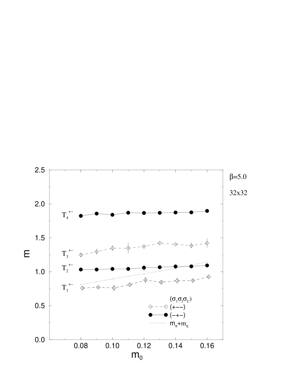
Figure 10: Pseudoscalar triplets with ${\sigma_{G}}=+1$ ($I^{PG}=1^{-+}\equiv T^{-+}$) (left) and scalar triplets with ${\sigma_{G}}=-1$ ($I^{PG}=1^{+-}\equiv T^{+-}$) (right). The dotted lines represent the sum of the masses of those particles which might be possible decay products of the plotted states.

The masses of these states are above the masses of the three predicted mesons.

Many of these states might be unstable. For example, it follows from fig. 10 that the $T_{2}^{PG}=T_{2}^{-+}$–particle might decay into a $\pi$– and a $f_{0}$–meson. The states which are definitely stable in the examined parameter region are the $T_{1}^{-+}$–, $T_{1}^{+-}$– and the $S_{1}^{--}$–meson. That means that these particles do not have decay channels as far as the determined mesonic states are concerned. There might be other particles like triplets with quantum numbers (${\sigma_{P}}=+1$, ${\sigma_{G}}=+1$) which have only a slight overlap with the operators we used in our simulations.

In figs. 10 and 11 masses with $m>1$ are to be understood mainly qualitatively,

Figure 11: Left: Different particles on the lattice which correspond to singlet states in the continuum ($I^{PG}=0^{PG}\equiv S^{PG}$). Right: Complete overview of the measured states apart from the three light mesons $\pi$, $f_{0}$ and $\eta$.

because one expects substantial ${{\cal O}(a)}$–corrections.

Summarizing the results for the mass spectrum we see that we are able to identify the predicted mesons — $\pi$, $f_{0}$ and $\eta$ — and their masses in Monte–Carlo simulations. The analytical predictions for the scaling of the pion– and $f_{0}$–mass (see section 2.2) are confirmed with small deviations. Best results are obtained for $\beta=10$ whereas for $\beta\leq 5$ deviations from the continuum results occur. Considering the measurements for the various couplings the predictions from the sine–Gordon model for the strong coupling region of the Schwinger model are reliable for $m_{0}/e<0.25$.

Concerning the $\pi$–$\pi$ scattering those particles with $m\simeq 2m_{\pi}$ are of interest because they might occur as resonances in the elastic scattering processes or they might be confused with the two–pion–energies in finite volume as it will be shown in section 6.3.

6 Scattering phases

The aim of this section is to present the methods and results for the determination of the scattering phases for the elastic $\pi$–$\pi$ scattering in the Schwinger model. As already mentioned in the introduction we use a formula which was derived by Lüscher for massive quantum field theories [42, 1, 4, 3]. This method is based on the fact that for not too small volumes the energies of the two–particle states in finite volume are determined by the elastic S–matrix of the model in infinite volume. Therefore Lüscher’s method is suitable for the investigation of scattering processes on the lattice with Monte–Carlo simulations.

6.1 Lüscher’s method

The system we are interested in consists of two bosonic particles of mass $m$ in $1+1$ dimensions in a finite box with spatial length $L$. We work in the center–of–mass system with zero total momentum. The formula for the determination of the scattering phases $\delta$ for the elastic scattering of the particles in infinite volume was given in ref. [4]:

$$2\delta({\bf{k}})=-{\bf{k}}\,L\hskip 28.45274pt\mbox{mod $2\pi$}\hskip 4.30554pt.$$ (49)

${\bf{k}}$ is the momentum of one particle in the finite box in the center–of–mass system. It is related to the discrete two–particle energy $E$ by the relativistic formula:

$$E=2\sqrt{m^{2}+{\bf{k}}^{2}}\hskip 4.30554pt.$$ (50)

For a potential with short range it can be easily shown that equation (49) is exact in quantum mechanics [4]. Also for a bosonic scalar quantum field theory in four dimensions a relation between the scattering phases and the particle momenta in finite volume can be derived [3].

An exact derivation of (49) in an arbitrary quantum field theory is in general not possible. Nevertheless it is plausible that (49) holds provided that [4]

• the examined quantum field theory has no massless particles in its spectrum

• the mixing of the relevant two–particle states with other many–particle states is excluded

• the range of the two–particle interaction is much smaller than half the spatial extension.

In the sine–Gordon model no inelastic scattering processes exist [15]. Nevertheless such inelastic processes are possible in the Schwinger model. Therefore in the Schwinger model one has to ensure that the lowest two–particle energies are below the inelastic threshold $E=4m$. Furthermore, one has to guarantee that no production of other particles occurs in the relevant energy region.

If the extension of the spatial volume is too small, further exponentially decaying finite size effects (polarization effects) appear in the two–particle energies. This leads to corrections to formula (49). As far as the scattering phases are concerned it is difficult to determine numerically these finite size effects. To reduce these unwanted effects on the two–particle energies the minimum lattice size for all simulations is chosen so that the finite size effect for the pion mass is negligible.

6.2 Correlation functions

For the determination of the two–particle energies in the finite volume we start with the successful ansatz of refs. [4, 9, 12]. This means that we construct a correlation matrix with time–slice–operators where different operators are characterized by different orthogonal functions:

$$O_{i}^{LT_{\tau}}(t) = \frac{1}{L^{2}}\sum_{{\bf{x}},{\bf{y}}}{\phi_{{\bf{x}},{\bf{y}}}}{\bar{\chi}_{{\bf{x}},t}}{\chi_{{\bf{x}},t}}\,{\bar{\chi}_{{\bf{y}},t+\tau}}{\chi_{{\bf{y}},t+\tau}}\,\omega_{i}({\bf{y}}-{\bf{x}})\hskip 4.30554pt,$$ (54)

$$\hskip 28.45274pt{\phi_{{\bf{x}},{\bf{y}}}}=(\pm 1)^{\bf{x}}(\pm 1)^{\bf{y}},\,\,\tau=0,1\,,$$

$$\hskip 28.45274pt\omega_{i}({\bf{x}})=\left\{\begin{array}[]{l}\cos({\bf{p}}_{i}{\bf{x}})\\ \sin({\bf{p}}_{i}{\bf{x}})\,,\hskip 14.22636pt{\bf{p}}_{i}=\frac{2\pi}{L}i,\;\;i=0,1,\ldots\hskip 4.30554pt.\end{array}\right.$$

These operators having the property that the fermion and antifermion in each meson operator are local in time are denoted by $LT\equiv LT_{0}$ ($\tau=0$) and $LT_{1}$ ($\tau=+1$). The definition of the functions $\omega_{i}({\bf{x}})$ and ${\phi_{{\bf{x}},{\bf{y}}}}$ depends on the choice of the lattice symmetry sector. In some sectors it is also possible to use two definitions for ${\phi_{{\bf{x}},{\bf{y}}}}$: ${\phi_{{\bf{x}},{\bf{y}}}}\equiv(-{\sigma_{1}})^{\bf{x}}(-1)^{\bf{y}}$ or ${\phi_{{\bf{x}},{\bf{y}}}}\equiv{\sigma_{1}}^{\bf{x}}$. The corresponding operators are denoted with a $1$ and $2$ respectively appended to the quantum numbers.

The operator (54) has the quantum number ${\sigma_{C}}=+1$. To construct eigenstates on the lattice which are odd under charge conjugation we use

$$O_{i}^{NLT}(t)=\frac{1}{L^{2}}\sum_{{\bf{x}},{\bf{y}}}{\phi_{{\bf{x}},{\bf{y}}}}\,{\bar{\chi}_{{\bf{x}},t+1}}{\chi_{{\bf{x}},t}}\,{\bar{\chi}_{{\bf{y}},t}}{\chi_{{\bf{y}},t+1}}\,{U_{2}({\bf{x}},t)}{U^{\ast}_{2}({\bf{y}},t)}\omega_{i}({\bf{y}}-{\bf{x}})\hskip 4.30554pt,$$ (55)

which in general is not an eigenstate under charge conjugation. This is an operator where the fermion and antifermion in each meson are non–local in time ($NLT$). Like in the case of the $LT$-operators the definition of $\omega_{i}({\bf{y}}-{\bf{x}})$ and ${\phi_{{\bf{x}},{\bf{y}}}}$ is determined by the symmetry sector.

The advantage of the special construction (55) is visible if one constructs an operator with a definite quantum number ${\sigma_{C}}$:

$${O_{{\sigma_{C}},\,i}^{NLT}}(t) \equiv O_{i}^{NLT}(t)+{\sigma_{C}}\left({{\mathscr{C}}_{0}}O_{i}^{NLT}\right)(t)$$ (56)

$$= \sum_{{\bf{x}},{\bf{y}}}{\bar{\chi}_{{\bf{x}},t+1}}{\chi_{{\bf{x}},t}}\,{\bar{\chi}_{{\bf{y}},t}}{\chi_{{\bf{y}},t+1}}\,{U_{2}({\bf{x}},t)}{U^{\ast}_{2}({\bf{y}},t)}\omega_{i}({\bf{y}}-{\bf{x}})$$

$$\hskip 142.26378pt{\bf\cdot}\left\{{\phi_{{\bf{x}},{\bf{y}}}}+{\sigma_{C}}{\sigma_{I}}{\phi_{{\bf{y}},{\bf{x}}}}\right\}\hskip 4.30554pt.$$

Because of the expression (56) the calculation of Green–functions with the $NLT$–operator is not more expensive than the calculation with the $LT$–operator.

As it will be shown in the following section the four–meson correlation functions of the operators (54) and (55) include contributions from one–particle states. To avoid such contributions for the determination of the $\pi$–$\pi$ scattering phases it appears advisable to calculate correlation functions which are constructed according to the $(I=2)$–sector in the continuum because there no one–particle states occur. Details will be seen in section 6.3. The procedure of the derivation of these correlation functions is the same as for the ${C_{\pi}}$–function: The starting–point here are the expectation values $C_{cont,ij}(t)=\langle O_{i}(t)\tilde{O}_{j}(t)\rangle$ in the continuum. The operators $O_{i}$ and $\tilde{O_{j}}$ are defined by

$$O_{i}(t) \equiv \frac{1}{(2\pi)^{2}}\int d{\bf{x}}d{\bf{y}}\,\omega_{i}({\bf{y}}-{\bf{x}}){\bar{\psi}}^{1}({\bf{x}},t)\gamma_{5}\psi^{2}({\bf{x}},t)\,{\bar{\psi}}^{1}({\bf{y}},t)\gamma_{5}\psi^{2}({\bf{y}},t)\,,$$

$$\tilde{O}_{j}(t) \equiv \frac{1}{(2\pi)^{2}}\int d{\bf{x}}d{\bf{y}}\,\omega_{j}({\bf{y}}-{\bf{x}}){\bar{\psi}}^{2}({\bf{x}},t)\gamma_{5}\psi^{1}({\bf{x}},t)\,{\bar{\psi}}^{2}({\bf{y}},t)\gamma_{5}\psi^{1}({\bf{y}},t)\hskip 4.30554pt.$$

By naive translation of the correlation functions $C_{cont,ij}(t)$ into the lattice formulation one obtains among others the following terms

$$C_{\pi\pi,ij}(t)$$

$$\equiv \frac{{\sigma_{I}}}{L^{3}}\sum_{{\bf{x}},{\bf{y}},{\bf{z}}}{\langle}\,|{M^{-1}({\bf 1},{\bf 3})}|^{2}\,|{M^{-1}({\bf 2},{\bf 4})}|^{2}+|{M^{-1}({\bf 2},{\bf 3})}|^{2}\,|{M^{-1}({\bf 1},{\bf 4})}|^{2}$$

$$-2\mbox{Re}\left[{M^{\ast-1}({\bf 1},{\bf 4})}\,{M^{-1}({\bf 1},{\bf 3})}\,{M^{\ast-1}({\bf 2},{\bf 3})}\,{M^{-1}({\bf 2},{\bf 4})}\right]\,{\rangle}_{U}$$

$${\bf\cdot}(-1)^{{\bf 1}+{\bf 2}+{\bf 3}+{\bf 4}}\,\omega_{i}({\bf{y}}-{\bf{x}})\omega_{j}({\bf{z}})\,{\phi_{{\bf{x}},{\bf{y}}}}{\phi_{{\bf{z}},0}}\,,$$

$$\hskip 28.45274pt\mbox{${\bf 1}\equiv({\bf{x}},t),\hskip 28.45274pt{\bf 2}\equiv({\bf{y}},t+\tau)$},$$

$$\hskip 28.45274pt\mbox{${\bf 3}\equiv({\bf{z}},0),\hskip 28.45274pt{\bf 4}\equiv(0,\tau^{\prime})$}\hskip 4.30554pt.$$

The prefactors in (6.2) are chosen in such a way that the expression (6.2) coincides with corresponding terms in the correlation function of the operators (54). In the following the index $\mbox{}_{\pi\pi}$ always denotes a correlation function of the type (6.2). For $\tau=\tau^{\prime}=0,1$ the expression (6.2) is related to the $LT$,$LT_{1}$–operator and for $\tau=1$, $\tau^{\prime}=0$ to an $LT_{1}$–$LT$ correlation function. If one takes the naive continuum limit of these lattice correlation functions it turns out that only the expression (6.2) contributes to the expectation values $C_{cont,ij}(t)$. Hence we expect the $C_{\pi\pi}(t)$–function to yield the dominant contribution to the $I=2$ continuum sector and therefore to be sufficient to calculate the two–particle energies in this sector.

The advantage of the expression (6.2) is obvious. Compared to the calculation of e.g. $\langle O^{LT}(t)O^{LT}(0)\rangle$ the calculation of (6.2) needs merely a fraction of the conjugate gradient calculations.

6.3 One–particle states in four–meson correlation functions

The numerical results for the four–meson correlation functions with the operators (54) and (55) show that in nearly all sectors the main contributions and hence the lowest energies can be identified with the single–particle masses of the model. Just as for the two–meson correlation functions the pion–state here also occurs with the best signal–to–noise ratio. The comparison of the determined masses with the pion–mass calculated with the two–pion correlation function ${C_{\pi}}(t)$ shows a good correspondence between the results for the two–meson and four–meson correlation functions (see fig. 12).

Figure 12: Results for the pion mass for different four–meson correlation functions in different lattice sectors. The dashed line is a fit to the data, whereas the solid line represents the mass obtained from the two–pion correlation function ${C_{\pi}}$.

This result can be explained in terms of the general properties of the SU(2) flavour group of the Schwinger model: The structure of the group SU(2) is such that some irreducible representations may be expressed either in terms of tensors of rank four or tensors of rank two. Therefore it is possible to examine properties of particles with isospin $1$, i.e. triplets, with fermionic eight–point functions. According to table 1 the lattice sectors which are connected to a $I^{PG}=1^{-+}$ continuum state are $({\sigma_{1}},{\sigma_{I}},{\sigma_{C}})$ = $(--+)$, $(-++)$ and $(+++)$. In fact we observe the pion in all these sectors (see fig. 12). Besides the pion we have determined also other mesons — the $f_{0}$– and $T_{1}^{+-}$–meson — with appropriate fermionic eight–point functions.

According to table 1 the pion as well as the $\pi$–$\pi$ states occur in most sectors with ${\sigma_{C}}=+1$. Therefore the lowest energy and consequently (presumably) also the signal–to–noise ratio in these sectors is dominated by the pion. Furthermore, according to the results of section 5.4 there exist pseudoscalar mesons with masses $m\simeq 2m_{\pi}$. These particles possibly could make the determination of the two–particle energies more difficult. To avoid these problems we used for the reasons given above the $C_{\pi\pi}(t)$–function (6.2) for the determination of the scattering phases. In fact the numerical results discussed in section 6.5 show that by using the $C_{\pi\pi}(t)$–function the contributions of the single–particle states are suppressed. In particular the lowest energies in the $C_{\pi\pi}(t)$–function are the $\pi$–$\pi$ energies.

6.4 Connected correlation functions

One might suspect that the only cause for the appearance of the one–particle energies in some four–meson correlation functions are poles in the disconnected parts of the correlation functions. To refute this hypothesis we examined a four–meson correlation function $C_{ij}(t)=\left\langle\,O_{i}^{LT}(t)O_{j}^{LT}(0)\,\right\rangle$. (The following discussion also holds for other operators ($LT_{1}$, $NLT$, …) with more general space–time arguments of the fermions.) This correlation function separates into a sum of connected correlation functions and disconnected parts:

$$C_{ij}(t)=\raisebox{-17.0pt}{ \begin{picture}(40.0,40.0)\immediate\ignorespaces\immediate\ignorespaces\immediate\ignorespaces\immediate\ignorespaces\immediate\ignorespaces{\immediate\immediate}\put(0.0,0.0){{\f@ynmf:feynfmf\char 1\relax}}\ignorespaces\immediate\ignorespaces\immediate\ignorespaces\immediate\ignorespaces\immediate\ignorespaces\immediate\ignorespaces\immediate\ignorespaces\immediate\ignorespaces\immediate\ignorespaces\immediate\ignorespaces \immediate\ignorespaces{}\end{picture} \ }\ +\mbox{disconnected graphs}\hskip 4.30554pt.$$ (58)

The shaded symbol represents the connected Green–function ($\langle\ldots\rangle_{c}$). The external legs denote quark–antiquark pairs in which the incoming mesons on the left live on the time slice $t$ and the outgoing mesons on the right on the time slice $0$.

The disconnected parts consist of

$$\raisebox{-17.0pt}{ \begin{picture}(40.0,40.0)\immediate\ignorespaces\immediate\ignorespaces\immediate\ignorespaces\immediate\ignorespaces\immediate\ignorespaces{\immediate\immediate}\put(0.0,0.0){{\f@ynmf:feynfmf\char 2\relax}}\ignorespaces\immediate\ignorespaces\immediate\ignorespaces\immediate\ignorespaces\immediate\ignorespaces\immediate\ignorespaces\immediate\ignorespaces\immediate\ignorespaces\immediate\ignorespaces\immediate\ignorespaces\immediate\ignorespaces\immediate\ignorespaces \immediate\ignorespaces{}\end{picture}}_{({\bf A})}\ +\ \raisebox{-17.0pt}{ \begin{picture}(40.0,40.0)\immediate\ignorespaces\immediate\ignorespaces\immediate\ignorespaces\immediate\ignorespaces\immediate\ignorespaces{\immediate\immediate}\put(0.0,0.0){{\f@ynmf:feynfmf\char 3\relax}}\ignorespaces\immediate\ignorespaces\immediate\ignorespaces\immediate\ignorespaces\immediate\ignorespaces\immediate\ignorespaces\immediate\ignorespaces\immediate\ignorespaces\immediate\ignorespaces\immediate\ignorespaces\immediate\ignorespaces\immediate\ignorespaces \immediate\ignorespaces{}\end{picture}}_{({\bf B})}\ +\ \raisebox{-12.0pt}{ \begin{picture}(30.0,30.0)\immediate\ignorespaces\immediate\ignorespaces\immediate\ignorespaces\immediate\ignorespaces\immediate\ignorespaces{\immediate\immediate}\put(0.0,0.0){{\f@ynmf:feynfmf\char 4\relax}}\ignorespaces\immediate\ignorespaces\immediate\ignorespaces\immediate\ignorespaces\immediate\ignorespaces\immediate\ignorespaces\immediate\ignorespaces\immediate\ignorespaces \immediate\ignorespaces{}\end{picture}}\raisebox{-12.0pt}{ \begin{picture}(30.0,30.0)\immediate\ignorespaces\immediate\ignorespaces\immediate\ignorespaces\immediate\ignorespaces\immediate\ignorespaces{\immediate\immediate}\put(0.0,0.0){{\f@ynmf:feynfmf\char 5\relax}}\ignorespaces\immediate\ignorespaces\immediate\ignorespaces\immediate\ignorespaces\immediate\ignorespaces\immediate\ignorespaces\immediate\ignorespaces\immediate\ignorespaces \immediate\ignorespaces{}\end{picture}}_{({\bf C})}$$ (59)

and of graphs like

$$\raisebox{-17.0pt}{ \begin{picture}(40.0,40.0)\immediate\ignorespaces\immediate\ignorespaces\immediate\ignorespaces\immediate\ignorespaces\immediate\ignorespaces{\immediate\immediate}\put(0.0,0.0){{\f@ynmf:feynfmf\char 6\relax}}\ignorespaces\immediate\ignorespaces\immediate\ignorespaces\immediate\ignorespaces\immediate\ignorespaces\immediate\ignorespaces\immediate\ignorespaces\immediate\ignorespaces\immediate\ignorespaces\immediate\ignorespaces \immediate\ignorespaces{}\end{picture}}{\bf\cdot}\,\ldots\hskip 4.30554pt.$$ (60)

The dots in (60) represent graphs with three external legs like   .

In the usual procedure only the vacuum parts $({\bf A})$ are subtracted from the Green–function to obtain the connected Green–function

$$\left\langle\,O_{i}(t)O_{j}(0)\,\right\rangle_{c}\simeq\left\langle\,O_{i}(t)O_{j}(0)\,\right\rangle-\left\langle\,O_{i}(t)\,\right\rangle\left\langle\,O_{j}(0)\,\right\rangle\hskip 4.30554pt.$$ (61)

In our simulations it turns out that the expressions $({\bf B})$ and $({\bf C})$ are not negligible and must also be subtracted in eq. (61). However it can be derived easily that $({\bf B})$ as well as $({\bf C})$ disappear for $i\neq j$ because of the orthogonality of the functions $\omega_{i}({\bf{y}}-{\bf{x}})$. For example, the term $({\bf B})$:

$$({\bf B}) \propto \sum_{{\bf{x}},{\bf{y}},{\bf{x}^{\prime}},{\bf{y}^{\prime}}}{\phi_{{\bf{x}},{\bf{y}}}}\omega_{i}({\bf{y}}-{\bf{x}})\omega_{j}({\bf{y}^{\prime}}-{\bf{x}^{\prime}})$$ (62)

$${\bf\cdot}\left\langle\,{\bar{\chi}_{{\bf{x}},t}}{\chi_{{\bf{x}},t}}\,{\bar{\chi}_{{\bf{x}^{\prime}},t_{0}}}{\chi_{{\bf{x}^{\prime}},t_{0}}}\,\right\rangle\left\langle\,{\bar{\chi}_{{\bf{y}},t}}{\chi_{{\bf{y}},t}}\,{\bar{\chi}_{{\bf{y}^{\prime}},t_{0}}}{\chi_{{\bf{y}^{\prime}},t_{0}}}\,\right\rangle$$

can be rewritten to obtain

$$({\bf B}) \propto \delta_{ij}\frac{L^{2}}{2}\sum_{{\bf{x}}}{\phi_{1,{\bf{x}}}}\cos({\bf{p}}_{i}{\bf{x}})\left\langle\,{\bar{\chi}_{{\bf{x}},t}}{\chi_{{\bf{x}},t}}\,{\bar{\chi}_{0,t_{0}}}{\chi_{0,t_{0}}}\,\right\rangle$$

$${\bf\cdot}\sum_{{\bf{y}}}{\phi_{2,{\bf{y}}}}\cos({\bf{p}}_{i}{\bf{y}})\left\langle\,{\bar{\chi}_{{\bf{y}},t}}{\chi_{{\bf{y}},t}}\,{\bar{\chi}_{0,t_{0}}}{\chi_{0,t_{0}}}\,\right\rangle\hskip 4.30554pt,$$

$$\hskip 28.45274pt{\phi_{{\bf{x}},{\bf{y}}}}{=:}\,{\phi_{1,{\bf{x}}}}{\phi_{2,{\bf{y}}}}\hskip 4.30554pt,\hskip 28.45274pti\neq 0,\frac{L}{2}\hskip 4.30554pt.$$

In the same way one obtains $({\bf C})\propto\delta_{ij}$. This means that the disconnected parts $({\bf B})$ and $({\bf C})$ contribute to the diagonal elements of the correlation matrix only.

This result shows that the one–particle contributions to the four–meson correlation functions can not come from the terms in (59) only, because we obtain in our simulations that the pion state also occurs in the non–diagonal elements of the correlation matrices (see table 2).

$$\left(\begin{array}[]{llll}0.503(14)&0.506(6)&0.492(6)&0.498(17)\\ 0.505(4)&0.50(2)&0.504(12)&0.516(6)\\ 0.498(2)&0.50(4)&0.495(9)&0.523(9)\\ 0.494(2)&0.51(4)&0.495(9)&0.526(9)\end{array}\right)$$ (68)

Table 2: Pion–masses which result from each of the $16$ matrix elements for a $4\times 4$ correlation matrix. The values are obtained with an $LT$ operator for $\beta=5.0$, $m_{0}=0.16$ and $L\times T=24\times 64$ in the sector $({\sigma_{1}},{\sigma_{I}},{\sigma_{C}})$ = $(--+)_{2}$. For comparison: The pion–mass for a single–particle operator is $m_{\pi}=0.4991(3)$.

Actually, the disconnected parts are a nuisance for the determination of two–meson energies: From equation (6.4) it follows that the disconnected parts are products of propagators of moving mesons. Therefore from (6.4) one obtains energies which are twice the energy of a single free meson with momentum ${\bf{p}}_{i}$. In fact we could determine these energies with a good signal in the Green–function $C_{ij}(t)$. The overall results for $C_{ij}(t)$ as well as the measured energies from the disconnected parts $({\bf B})+({\bf C})$ alone are listed in table 3. Comparing the energies which correspond to each other from both measurements good agreement within the errors is visible.

These energies from the disconnected parts make it more difficult to analyse the simulation data and to determine two–meson energies we are mainly interested in. In some cases they might even be confused with the two–pion energies. In order to avoid contributions from the expressions $({\bf B})$ and $({\bf C})$ we considered only correlations with $i\neq j$, because as we have seen above all non–diagonal elements of $({\bf B})$ and $({\bf C})$ vanish. In fact we calculated $r\times r$ correlation matrices $D(t)$ which are not symmetric in their indices:

$$D_{ij}(t) {:=} C_{i,r+j}(t)$$ (69)

$$= \left\langle\,O_{i}(t)O_{r+j}(0)\,\right\rangle,\hskip 28.45274pti,j=1\ldots r\hskip 4.30554pt.$$

Moreover, we did not use momenta ${\bf{p}}_{i}=0,\pi$ for the wave functions. In this case it can be shown that the contributions from (60) vanish, too.

Altogether we use the function $D_{\pi\pi}(t)$ for the calculation of the two–pion energies. This is a correlation matrix (69), for which according to (6.2), only those parts contribute which are relevant for the $\pi$–$\pi$ scattering in the $(I=2)$–sector.

	$C_{ij}(t)$	$(\bf B)+(\bf C)$	$2E_{bos}(m_{\pi},{\bf{p}}_{i})$
$m_{\pi}$	$0.506(5)$	—–	—–
Energy $E_{2}$	$1.10(3)$	$1.21(4)$	$1.124(9)$
Energy $E_{3}$	$1.53(11)$	$1.49(3)$	$1.418(7)$
Energy $E_{4}$	$1.89(16)$	$1.89(4)$	$1.776(5)$

Table 3: Comparison of the results from the four–meson correlation matrix $C_{ij}(t)$ with the values resulting from the disconnected parts $(\bf B)+(\bf C)$. The energies were obtained for the same simulation parameters $\beta=5.0$, $m_{0}=0.16$, $L\times T=24\times 64$ from a $4\times 4$ correlation matrix. Additionally the energies which were calculated with the bosonic dispersion relation are listed ($m_{\pi}=0.506(5)$, ${\bf{p}}_{i}=2\pi i/L$, $i=1\ldots 3$).

Analyzing the numerical data for $D_{\pi\pi}(t)$ it turns out that the best results are not obtained by calculating the generalized eigenvalues but just by diagonalizing the correlation matrix. In this case the eigenvalues show the following behaviour ($T\rightarrow\infty$):

$$\lambda_{l}(t)\stackrel{{\scriptstyle t\rightarrow\infty}}{{=}}c_{l}(\sigma_{l})^{t}\,{e^{-tE_{l}}}\left[1+{{\cal O}({e^{-t\Delta E_{l}}})}\right]\,,\hskip 14.22636pt\sigma_{l}=\pm 1\hskip 4.30554pt.$$ (70)

Like in eq. (19) $\Delta E_{l}$ denotes the smallest difference between $E_{l}$ and other spectral energies. Following closely the proof in ref. [4], equation (70) can be derived easily for the $D_{\pi\pi}(t)$–correlation matrix.

6.5 Results for the scattering phases

For the determination of the two–particle energies we calculated a $4\times 4$ $D_{\pi\pi}(t)$–matrix with the $LT$–, $LT_{1}$–operators (see section 6.2) and the $LT_{1}$–$LT$ operator combination for all relevant lattice sectors. The simulation results show that a clear signal for the $\pi$–$\pi$ energies occurs only for the $LT$–operator in the $({\sigma_{1}},{\sigma_{I}},{\sigma_{C}})$ = $(+++)_{2}$ lattice sector. For the calculation of the energies in this case it was frequently necessary to enlarge the correlation matrix to obtain a better separation of the different energies. Hence we extracted the lowest energy only whereas higher energies could not be determined with sufficient accuracy.

To improve the signal for the lowest energy we use smeared operators (see section 5.1). The optimal value for the smearing parameter $\alpha$ from simulations with low statistics turned out to be $\alpha\simeq 0.02$. Here one has to be aware of the fact that the replacement of the antifermions in a two–meson operator $O(t)$ with quantum number ${\sigma_{C}}(O)$ by smeared antifermions (“smeared source”) leads to a smeared operator $O^{S}(t)$ which has no definite behaviour under charge conjugation. In such cases it is useful to chose $\alpha$ so small to have dominant contributions from the sector with ${\sigma_{C}}={\sigma_{C}}(O)$.

The results for the lowest eigenvalues of two typical correlation matrices are shown in fig. 13.

Figure 13: Two–particle energies for ($\beta=10$, $m_{0}=0.11$ ) for two different spatial extensions of the lattice in the sector $({\sigma_{1}},{\sigma_{I}},{\sigma_{C}})=(+++)_{2}$. The lowest eigenvalue of the correlation matrix and its effective energy are plotted.

Sufficiently good plateaus in the effective energies are obtained for relatively high values of the time argument $t$. For small values of $t$ the eigenvalues show a qualitatively different behaviour. Therefore the calculation of generalized eigenvalues is not successful here, because for the method of generalized eigenvalues the reference time $t_{0}$ of equation (3.2) has to be chosen small to reduce the statistical errors.

For the $D_{\pi\pi}(t)$–function the use of smeared sources is not as advantageous as for the two–pion correlation function ${C_{\pi}}(t)$. Despite smearing the matrix elements of the subtracted function $D^{LT}_{S,\pi\pi}(t){:=}D^{LT}_{\pi\pi}(t)-D^{LT}_{\pi\pi}(t+2)$ for $t=10$ and $(\beta=10,m_{0}=0.11)$ have a bad signal–to–noise ratio of about $0.02$ to $0.08$. The subtracted correlation function is used here in order to avoid any contributions from constant terms. The signal–to–noise ratio above has to be compared with the signal–to–noise ratio of $4.18(2)$ for the subtracted function ${C_{S,\pi}}(t){:=}{C_{\pi}}(t)-{C_{\pi}}(t+2)$ with $\alpha=0.1$. Therefore we had to generate for each point a minimum of $65000$ independent configurations to reduce the statistical errors of the two–pion energies to about $1\%$.

The comparison of the $D^{LT}_{\pi\pi}(t)$–function with the correlation function $C^{LT}(t)\equiv\langle O_{i}^{LT}(t)O_{i}^{LT}(0)\rangle$ justifies the usage of the former function: The ratio $D^{LT}_{\pi\pi,ij}(t)/C^{LT}_{ij}(t)$ of the matrix elements of both functions for the parameters given above is less than $10^{-3}$. This means that the $D^{LT}_{\pi\pi}(t)$ parts of the $C^{LT}(t)$–correlation function are strongly suppressed. Thus it is appropriate to use the correlations $D^{LT}_{\pi\pi}(t)$ from the beginning.

The scattering phases which were calculated from the two–particle energies by the bosonic dispersion relation (46) are shown in figs. 14 and 15.

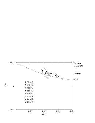
Figure 14: Scattering phases for two different bare masses and different lattice sizes. The analytical prediction for the $\pi$–$\pi$ scattering according to eq. (9) is represented by the solid curve. The mass of the scattered pions is $m_{\pi}=0.2545(10)$ and $m_{\pi}=0.3367(6)$ respectively. The solid/dotted bars in the lower diagram are the statistical errors of the data for $T=48/T=64$.

Figure 15: Scattering phases for $\beta=10$ and $m_{0}=0.14$. The pion mass is $m_{\pi}=0.4010(2)$.

In fig. 14 the numerical values confirm well within errors the analytical prediction (9) for the $\pi$–$\pi$ scattering. This means that in both cases ($\beta=10$, $m_{0}=0.075$) and ($\beta=10$, $m_{0}=0.11$) for a ratio $m_{0}/e\equiv m_{0}\sqrt{\beta}$ of $0.24$ and $0.35$ respectively the strong–coupling prediction describes the data very well. Therefore the analytical strong–coupling prediction for the elastic $\pi$–$\pi$ scattering phases in the Schwinger model as resulting from the sine–Gordon model are confirmed.

If the ratio $m_{0}/e$ is increased further to $m_{0}/e=0.44$ for ($\beta=10$, $m_{0}=0.14$) it becomes obvious from fig. 6 that the prediction (9) is no longer valid. Indeed the lowest numerical determined scattering phases in fig. 15 lie below the analytical curve. Considering our numerical results for the mass spectrum these deviations can not result from inelastic processes. The threshold for possible inelastic processes like $\pi\pi\rightarrow\eta\eta$ or $\pi\pi\rightarrow f_{0}f_{0}$ for the parameters in question is far above the determined two–particle energies. Furthermore, we did not find any particles, e.g. ($I^{PG}=0^{++}$)–mesons, which might occur as resonances in the examined energy region and the lattice sectors considered. Therefore the deviations in fig. 15 can not be caused by resonances in the elastic scattering channel.

Because there are no inelastic thresholds near or below respectively the calculated energies we can conclude that the investigated pion–pion state is a definite two–particle state which does not mix with other many–particle states. Therefore according to section 6.1 the applicability of Lüscher’s method is guaranteed. Within the statistical errors the numerical results do not indicate that it is necessary to consider any CDD–factors for the elastic pion–pion scattering. Nevertheless it is possible to multiply the “minimal” solution (9) with CDD–factors of the type (11), e.g. two factors with $\alpha_{1}\simeq-\alpha_{2}$, without changing the shape of the scattering phases qualitatively.

7 Summary

In this paper we present the mass spectrum of light mesons in the massive Schwinger model with an ${\mbox{SU(2)}}_{f}$ flavour symmetry. Furthermore, Lüscher’s method is successfully applied to the calculation of mesonic scattering phases in this model. For strong coupling the analytical predictions for the pion mass and for the elastic scattering phases of the pion–pion scattering are confirmed.

Investigating the mass spectrum in the Schwinger model it is shown that for $\beta=10$ and for small bare fermion masses $m_{0}$ the dependence of the pion mass on the bare parameters corresponds to the analytical predictions. A significant improvement of the data is achieved compared to the results for $\beta=4$ [25]. This was expected as the continuum limit requires $\beta\rightarrow\infty$.

The $f_{0}$ and $\eta$ singlet states which are analytically predicted in addition to the pion are investigated in the strong coupling region, i.e. for small values of $m_{0}\sqrt{\beta}$. The numerical results for the mass of the $f_{0}$–meson are for $\beta=5$ and $\beta=7$ in the region of the analytically predicted value of $m_{f_{0}}=\sqrt{3}\,m_{\pi}$. The mass of the $\eta$–meson is predicted to be $m_{\eta}=e\sqrt{2/\pi}$ in the massless ${\mbox{SU(2)}}_{f}$ Schwinger model ($e$ is the coupling parameter in the continuum). We find in the massive case that there are corrections to this value which are linear in $m_{0}$.

Additionally in the mass region $[m_{\pi},4m_{\pi}]$ we find a rich mass spectrum consisting of scalar and pseudoscalar triplet and singlet states. We assume the lightest of these particles to be stable.

The results for the elastic scattering phases of the pion–pion scattering show that the relevant two–pion states have only a slight overlap with the operators considered. In fact the signal–to–noise ratio of the correlation function used is below $10\%$ despite smearing. To improve the separation of the pion–pion energies from other states with large amplitude we use improved techniques like specific correlation functions for the two–pion states and enlarged correlation matrices. In this way it is possible to obtain scattering phases for the elastic pion–pion scattering using the method of Lüscher. For strong coupling these scattering phases are in good agreement with the analytical predictions.

The experience gained in this project may be useful for the calculation of elastic scattering phases in other gauge field theories. It turns out that the investigation of scattering processes with composite particles like mesonic states is much more difficult than the scattering of particles which are no bound states. This is in agreement with investigations of other fermionic models [43, 44, 11]. The main problem is the poor overlap of the two–meson states with the conventional operators. To compensate for this we had to generate up to $100000$ independent configurations per simulation point. Therefore the development of improved operators should be the main task for investigations of mesonic scattering processes in QCD by Lüscher’s method, e.g. of the $\rho$–resonance in a $\pi$–$\pi$ scattering.

References

- [1] M. Lüscher, Commun. Math. Phys. 105 (1986) 153.
- [2] M. Lüscher, Nucl. Phys. B 364 (1991) 237.
- [3] M. Lüscher, Nucl. Phys. B 354 (1991) 531.
- [4] M. Lüscher and U. Wolff, Nucl. Phys. B 339 (1990) 222.
- [5] J. Nishimura, Phys. Lett. B 294 (1992) 375.
- [6] C.R. Gattringer, I. Hip and C.B. Lang, Nucl. Phys. B (Proc. Suppl.) 30 (1993) 875.
- [7] C.R. Gattringer and C.B. Lang, Nucl. Phys. B 391 (1993) 463.
- [8] M. Göckeler, H.A. Kastrup, J. Westphalen and F. Zimmermann, Nucl. Phys. B (Proc. Suppl.) 34 (1994) 566.
- [9] M. Göckeler, H.A. Kastrup, J. Westphalen and F. Zimmermann, Nucl. Phys. B 425 (1994) 413.
- [10] S. Gottlieb and K. Rummukainen, Nucl. Phys. B 450 (1995) 397.
- [11] J. Westphalen, PhD thesis, Institut für Theoretische Physik E, RWTH Aachen, 1997.
- [12] M. Göckeler, H.A. Kastrup, J. Viola and J. Westphalen, Nucl. Phys. B (Proc. Suppl.) 47 (1996) 831.
- [13] R.F. Dashen, B. Hasslacher and A. Neveu, Phys. Rev. D 11 (1975) 3424.
- [14] A.B. Zamolodchikov, Int. J. Mod. Phys. A 10 (1995) 1125.
- [15] A.B. Zamolodchikov and A.B. Zamolodchikov, Ann. Phys. 120 (1979) 253.
- [16] C.R. Gattringer, Ann. Phys. 250 (1996) 389.
- [17] L.V. Belvedere, J.A. Swieca, K.D. Rothe and B. Schroer, Nucl. Phys. B 153 (1979) 112.
- [18] S. Coleman, Phys. Rev. D 11 (1975) 2088.
- [19] S. Coleman, Ann. Phys. 101 (1976) 239.
- [20] D.J. Gross, I.R. Klebanov, A.V. Matytsin and A.V. Smilga, Nucl. Phys. B 461 (1996) 109.
- [21] A.V. Smilga, Phys. Rev. D 55 (1997) 443.
- [22] M. Lüscher, Commun. Math. Phys. 85 (1982) 39.
- [23] C. Panagiotakopoulos, Nucl. Phys. B 251 (1985) 61.
- [24] C.R. Gattringer, I. Hip and C.B. Lang, Phys. Lett. B 409 (1997) 371.
- [25] C. Gutsfeld, H.A. Kastrup, K. Stergios and J. Westphalen, Nucl. Phys. B (Proc. Suppl.) 63 (1998) 266.
- [26] K. Stergios, PhD thesis, in preparation.
- [27] S. Elser and B. Bunk, hep–lat/9710019.
- [28] H. Dilger, Int. J. Mod. Phys. C 6 (1995) 123.
- [29] P. de Forcrand, J.E. Hetrick, T. Takaishi and A.J. van der Sijs, Nucl. Phys. B (Proc. Suppl.) 63 (1998) 679.
- [30] H. Dilger, DESY, Hamburg, 1993, Report 93-181.
- [31] G.W. Kilcup and S.R. Sharpe, Nucl. Phys. B 283 (1987) 493.
- [32] M.F.L. Golterman and J. Smit, Nucl. Phys. B 245 (1984) 61.
- [33] M.F.L. Golterman and J. Smit, Nucl. Phys. B 255 (1985) 328.
- [34] M.F.L. Golterman, Nucl. Phys. B 273 (1986) 663.
- [35] M. Göckeler, H.A. Kastrup, J. Viola and J. Westphalen, Nucl. Phys. B (Proc. Suppl.) 42 (1995) 782.
- [36] H. Kluberg–Stern, A. Morel, O. Napoly and B. Petersson, Nucl. Phys. B 220 (1983) 447.
- [37] R. Altmeyer, K.D. Born, M. Göckeler, R. Horsley, E. Laermann and G. Schierholz, Nucl. Phys. B 389 (1993) 445.
- [38] S.R. Carson and R.D. Kenway, Ann. Phys. 166 (1986) 364.
- [39] C.R. Allton et al., Phys. Rev. D 47 (1993) 5128.
- [40] W. Franzki, PhD thesis, Institut für Theoretische Physik E, RWTH Aachen, 1997.
- [41] M. Lüscher, Progress in Gauge Field Theory, edited by G. ’t Hooft et al., Cargèse 1983, Plenum (New York), 1984.
- [42] M. Lüscher, Commun. Math. Phys. 104 (1986) 177.
- [43] H.R. Fiebig, A. Dominguez and R.M. Woloshyn, Nucl. Phys. B 418 (1994) 649.
- [44] J. Canosa and H.R. Fiebig, Phys. Rev. D 55 (1997) 1487.