AZPH-TH-99-03

BUTP-99-04

MPI-PhT/99-09

March 1999

Comparison of the O(3) Bootstrap $\sigma$-Model
with the Lattice Regularization at Low Energies

János Balog

Research Institute for Particle and Nuclear Physics

H-1525 Budapest 114, P.O.B. 49, Hungary

Max Niedermaier

Department of Physics, University of Pittsburgh

Pennsylvania 15260, U.S.A.

Ferenc Niedermayer

Institute for Theoretical Physics, University of Bern

Sidlerstrasse 5, CH-3012 Bern, Switzerland

Adrian Patrascioiu

Physics Department, University of Arizona

Tucson, AZ 85721, U.S.A.

Erhard Seiler and Peter Weisz

Max-Planck-Institut für Physik

Föhringer Ring 6, D-80805 München, Germany

Abstract

The renormalized coupling $g_{{\hbox{\sixrm R}}}$ defined through the connected 4-point function at zero external momentum in the non-linear O(3) sigma-model in two dimensions, is computed in the continuum form factor bootstrap approach with estimated error $\sim 0.3\%$. New high precision data are presented for $g_{{\hbox{\sixrm R}}}$ in the lattice regularized theory with standard action for nearly thermodynamic lattices $L/\xi\sim 7$ and correlation lengths $\xi$ up to $\sim 122$ and with the fixed point action for correlation lengths up to $\sim 12$. The agreement between the form factor and lattice results is within $\sim 1\%$. We also recompute the phase shifts at low energy by measuring the two-particle energies at finite volume, a task which was previously performed by Lüscher and Wolff using the standard action, but this time using the fixed point action. Excellent agreement with the Zamolodchikov S-matrix is found.

1 Introduction

The presently only known practical way to define a relativistic quantum field theory non-perturbatively in 4 dimensions is by using the lattice regularization. For example it is hoped that one will, once sufficiently powerful computers are available, be able to answer the question whether QCD is the correct theory of the strong interactions by studying the continuum limit of the lattice theory.

It is however notoriously difficult to control the continuum limit of a lattice theory. Analyses of lattice Feynman graphs, as initially performed by Symanzik [?], show that order by order in renormalized perturbation theory, physical quantities approach their continuum limit as integer powers in the lattice spacing (up to logarithmic corrections). However, since it is not known that such behavior controls the approach to the continuum limit in the full non-perturbatively defined theory, the invocation of such a power-law approach to extrapolate data produced in numerical simulation experiments has merely the status of a (plausible) working hypothesis. The integer nature of the powers adopted in studies of theories such as QCD, is considered to be connected to the widely expected property of asymptotic freedom. Here again, the very question whether the continuum limit of the lattice theory really describes an asymptotically free theory is highly non-trivial.

This work is part of an on-going effort of the present authors to test whether the “conventional wisdom” is correct in a simpler model, the non-linear O(3) sigma model in 2 dimensions. This model is, like QCD, perturbatively asymptotically free and also has instanton and superinstanton [?] solutions. It has however classically the additional beautiful property of being integrable; in particular there exist an infinite set of non-local conserved charges. Assuming that the quantum theory has a mass gap and the spectrum contains a vector multiplet of stable particles, the existence of such conserved charges in the quantum theory forbid particle production in scattering and, as shown by Lüscher [?] fixes the 2-particle S-matrix to that previously postulated by Zamolodchikov and Zamolodchikov (ZZ) [?] (up to CDD ambiguities).

All these properties were obtained starting from a formal Lagrangian, where one first computes off-shell $N$-point functions and goes on-shell via the LSZ formalism to obtain the S-matrix elements. The so-called form factor bootstrap (FFB) approach [?,?,?] proceeds in the other direction. One attempts to obtain off-shell information starting from the knowledge (postulate) of the stable particle spectrum and their S-matrix. In the first step one constructs the form factors of (composite) operators, satisfying all physical constraints (analyticity, generalized Watson theorem etc.) and then Green functions are obtained by saturating with a complete set of states. This is a program which is only feasible in a theory where there is no particle production (i.e. only in 2 dimensions). Even this program, for which there has recently been a lot of progress [?,?,?], involves mammoth effort.

Unfortunately since lattice regularization breaks these conservation laws and the FFB relies on some nontrivial assumptions, the expectation that the continuum limit of the lattice O(3) model coincides with the FFB is not guaranteed. A first investigation of this issue was by Lüscher and Wolff [?] who computed the phase shifts on the lattice by measuring two particle state energies in finite volume. Their results (taking account of lattice artifacts) were completely consistent with the ZZ S-matrix. In the course of a similar investigation of the nature of the continuum limit of the O(2) model [?], in order to test our programs and a slightly modified form of the analysis, we repeated the measurement of the phase shifts in the O(3) model. We also made simulations with a fixed point action [?], and found indications that the lattice artifacts are much smaller than in the case of the standard action. An account of our investigations is given in sect. 4. Our results are again in good agreement with the ZZ S-matrix [?].

An off-shell quantity of physical interest is the current-current (J-J) correlation function. It has been shown that J-J computed in the FFB approach [?,?] agrees well with conventional renormalized perturbation theory at high energies, at least up to $p/M\sim 10000$, when the analytical value of the ratio of the mass $M$ to the $\Lambda$-parameter [?] is used. Connected to this are two important inter-related properties; firstly the ZZ S-matrix shows an “on-shell form of AF”, in the sense that the phase shifts fall logarithmically to zero with the energy at high energy (see sect. 4). Secondly the thermodynamic Bethe ansatz, which is used to compute $M/\Lambda$, reproduces the 2-loop $\beta$-function coefficient. The agreement between the FFB and lattice computations of J-J is also within $\sim 1\%$ for the entire range of momenta up to $\sim 40M$.

Despite this wealth of circumstantial evidence for the validity of the conventional picture, there is still room for doubt. In particular in a recent paper, two of the present authors [?], assuming a certain form of the lattice artifacts, have found statistically significant deviations between the continuum limit of the lattice J-J correlation function and the FFB at low energies.

Unfortunately the J-J correlation function at low energies is a quantity which behaves qualitatively similarly to that in a free theory. It is plausible that a difference between two theories would manifest itself more clearly in a quantity which vanishes in the free theory e.g. the zero momentum coupling $g_{{\hbox{\sixrm R}}}$ defined through the connected 4-point function. There is an enormous literature on the computation of this quantity in the 2 (and higher) dimensional non-linear sigma models, see e.g. ref. [?] and references therein. The main new contribution of this paper, the computation of $g_{{\hbox{\sixrm R}}}$ by the FFB, is outlined in sect. 2. This is the first time that this method has been used to compute a 4-point function, and it is rather surprising that one is apparently able to get such a good approximation for $g_{{\hbox{\sixrm R}}}$.

In sect. 3 we present results on $g_{{\hbox{\sixrm R}}}$ using two different lattice regularizations, the standard action (including new high precision data on thermodynamic lattices at large correlation lengths) and the fixed point (FP) action. The nature of the approach to the continuum limit is not so clear, but whatever (reasonable) extrapolation is made, it agrees with the truncated FFB result better than $\sim 1\%$.

2 Computation of $g_{{\hbox{\sixrm R}}}$ in the continuum theory

There have been various approximation schemes to compute low energy (non-pertur-bative quantities) in the continuum formulation of the O$(n)$ models in two dimensions: the $g$–expansion [?], the $\epsilon$-expansion [?], and the $1/n$ expansion [?]. In this section we will present a new approximation using the form factor bootstrap.

2.1 Definitions

Consider a general continuum quantum field theory in two dimensions, in infinite volume, with global O($n$) symmetry. Let $\sigma^{a}(x)$, $a=1\dots n$ be a vector multiplet of (renormalized) Euclidean scalar fields with 2-point function

$$S^{a_{1}a_{2}}(x_{1},x_{2})=\langle\sigma^{a_{1}}(x_{1})\sigma^{a_{2}}(x_{2})\rangle\,.$$ (2.1)

The inverse of its Fourier transform

$$G(k)\delta^{a_{1}a_{2}}=\int{\rm d}^{2}xe^{ikx}S^{a_{1}a_{2}}(x,0)\,,$$ (2.2)

is assumed to have an expansion for small momenta

$$G(k)^{-1}=Z_{{\hbox{\sixrm R}}}^{-1}\Big{(}M_{{\hbox{\sixrm R}}}^{2}+k^{2}+O(k^{4})\Bigr{)}\,.$$ (2.3)

We denote the 4-point function by

$$S^{a_{1}a_{2}a_{3}a_{4}}(x_{1},x_{2},x_{3},x_{4})=\langle\sigma^{a_{1}}(x_{1})\sigma^{a_{2}}(x_{2})\sigma^{a_{3}}(x_{3})\sigma^{a_{4}}(x_{4})\rangle\,,$$ (2.4)

and the connected 4-point function

$$S_{c}^{a_{1}a_{2}a_{3}a_{4}}(x_{1},x_{2},x_{3},x_{4})=S^{a_{1}a_{2}a_{3}a_{4}}(x_{1},x_{2},x_{3},x_{4})-S^{a_{1}a_{2}}(x_{1},x_{2})S^{a_{3}a_{4}}(x_{3},x_{4})$$

$$-S^{a_{1}a_{3}}(x_{1},x_{3})S^{a_{2}a_{4}}(x_{2},x_{4})-S^{a_{1}a_{4}}(x_{1},x_{4})S^{a_{2}a_{3}}(x_{2},x_{3}).$$ (2.5)

Introducing the Fourier transform by

$$\widetilde{S}^{a_{1}a_{2}a_{3}a_{4}}(k_{1},k_{2},k_{3},k_{4})=\int\prod_{j=1}^{4}\left[{\rm d}^{2}x_{j}e^{ik_{j}x_{j}}\right]S^{a_{1}a_{2}a_{3}a_{4}}(x_{1},x_{2},x_{3},x_{4})\,,$$ (2.6)

and similarly $\widetilde{S}_{c}$ for the connected part, the conventional zero momentum (dimensionless) coupling (in two dimensions) is defined by

$$g_{{\hbox{\sixrm R}}}=-{M_{{\hbox{\sixrm R}}}^{2}\over G(0)^{2}}{1\over n^{2}}\sum_{a,b}G^{aabb}(0,0,0,0)\,,$$ (2.7)

where

$$\widetilde{S}_{c}^{a_{1}a_{2}a_{3}a_{4}}(k_{1},k_{2},k_{3},k_{4})=(2\pi)^{2}\delta^{(2)}(k_{1}+k_{2}+k_{3}+k_{4})G^{a_{1}a_{2}a_{3}a_{4}}(k_{1},k_{2},k_{3},k_{4})\,.$$ (2.8)

We will assume that the 2-point function has a spectral representation

$$G(k)=Z\int_{0}^{\infty}{\rm d}\mu{\rho(\mu)\over\mu^{2}+k^{2}}\,,$$ (2.9)

where the normalization constant $Z$ takes into account that, assuming that the spectrum of the theory contains a vector multiplet of stable particles of mass $M$, we normalize the spectral density $\rho$ so that the 1-particle contribution is

$$\rho^{(1)}(\mu)=\delta(\mu-M).$$ (2.10)

Then the coefficients appearing in the small momenta expansion above can be expressed as

$$Z_{{\hbox{\sixrm R}}}=Z{\gamma_{2}^{2}\over\delta_{2}}\,,$$ (2.11)

$${M_{{\hbox{\sixrm R}}}^{2}\over M^{2}}={\gamma_{2}\over\delta_{2}}\,,$$ (2.12)

where $\gamma_{2}$ and $\delta_{2}$ are the moments

$$\gamma_{2}=M^{2}\int{\rm d}\mu\,{\rho(\mu)\over\mu^{2}},$$ (2.13)

$$\delta_{2}=M^{4}\int{\rm d}\mu\,{\rho(\mu)\over\mu^{4}}\,.$$ (2.14)

Further the coupling $g_{{\hbox{\sixrm R}}}$ can be written as

$$g_{{\hbox{\sixrm R}}}=-{n+2\over n}{\gamma_{4}\over\gamma_{2}\delta_{2}}$$ (2.15)

where $\gamma_{4}$ is defined through

$$G^{a_{1}a_{2}a_{3}a_{4}}(0,0,0,0)={Z^{2}\gamma_{4}\over M^{6}}\left(\delta^{a_{1}a_{2}}\delta^{a_{3}a_{4}}+\delta^{a_{1}a_{3}}\delta^{a_{2}a_{4}}+\delta^{a_{1}a_{4}}\delta^{a_{2}a_{3}}\right)\,.$$ (2.16)

Strictly speaking, all observable physics (in a massive theory) is on-shell; different interpolating fields give the same results. Off-shell amplitudes of particular composite (and ‘elementary’) operators, are only of physical interest if they are sources of (idealized) infinitesimal weakly interacting probes. The fields are characterized by their various quantum numbers and their dimensions e.g. coded in the behavior of the 2-point function $G(k)$. The assumption eq.(2.9) corresponds to a limitation on the behavior of the associated spectral function $\rho(\mu)$ as $\mu\to\infty$. It is an implicit connection to the association of $\sigma^{a}(x)$ with a particular local field in the Lagrangian quantum field theory. In the non-linear $O(n)$ sigma model the ‘elementary’ field $\sigma^{a}(x)$ is characterized by its vanishing engineering dimension (in addition to being an isovector and spacetime scalar). We can therefore assume that the short distance singularities of its two-point function are sufficiently weak (only logarithmic) so that the spectral representation (2.9) holds without subtractions. Indeed, in the FFB approach, this uniquely defines (up to normalization) an operator $\hat{\sigma}^{a}(x)$, which has form factors that are not growing too fast at infinity so that the corresponding spectral density $\rho(\mu)$ vanishes fast enough for $\mu\to\infty$.

2.2 $1/n$- and $\epsilon$-Expansions

The leading order computations for the spectral integrals in the $1/n$-expansion have been performed in ref [?]

$$\gamma_{2}=1+0.00671941{1\over n}+O\left({1\over n^{2}}\right)\,,$$ (2.17)

$$\delta_{2}=1+0.00026836{1\over n}+O\left({1\over n^{2}}\right)\,,$$ (2.18)

and also for the coupling [?]

$$g_{{\hbox{\sixrm R}}}={8\pi\over n}\left(1-0.602033{1\over n}+O({1\over n^{2}})\right),$$ (2.19)

which gives the approximation $g_{{\hbox{\sixrm R}}}=6.70$ for the case $n=3$.

In the $g$-expansion one obtains $g_{{\hbox{\sixrm R}}}=6.66(6)$ [?] and the $\epsilon$-expansion $g_{{\hbox{\sixrm R}}}=6.55(8)$ [?]. Considering the rather short series in each case it is amazing how well the estimates by the various methods agree.

2.3 Form factor bootstrap computation for $n=3$

The form factor bootstrap aims at reconstructing $N$-point functions of local operators of integrable field theories from the knowledge of the spectrum of stable particles and their S-matrix. A description can be found in Smirnov’s book [?], the review of Karowski [?], a recent paper [?] and in various articles of two of the present authors  [?].

To our knowledge this is the first time that the method has been applied to the computation of 4-point functions. The computation is rather involved and here we will only give a very brief outline and present our results. The calculation in this and in other integrable models will be described in detail in a forthcoming paper [?].

We assume (as did the Zamolodchikov brothers in their construction of the S-matrix) that there are no bound states in the O($n$) models. Then the spectral density $\rho$ has an expansion over contributions from the intermediate states with an odd number of particles (due to internal parity symmetry)

$$\rho(\mu)=\sum_{k=0}^{\infty}\rho^{(2k+1)}(\mu)\,,$$ (2.20)

and correspondingly the spectral integrals

$$\gamma_{2}=1+\sum_{k=1}^{\infty}\gamma_{2}^{(2k+1)}\,,$$ (2.21)

$$\delta_{2}=1+\sum_{k=1}^{\infty}\delta_{2}^{(2k+1)}\,.$$ (2.22)

The form factors are given by Smirnov [?] for the O$(3)$ model and have been recomputed in [?]. For example the matrix element of the Minkowski operator $\hat{\sigma}^{a}(0)$ associated to the Euclidean field $\sigma^{a}$, connecting the vacuum to the 3-particle in-state with rapidities $\theta_{1}\geq\theta_{2}\geq\theta_{3}$, is given by

$$\langle 0|\hat{\sigma}^{a}(0)|a_{1},\theta_{1};a_{2},\theta_{2};a_{3},\theta_{3}\rangle^{\rm in}=\sqrt{Z}{\cal F}^{a}_{a_{1}a_{2}a_{3}}(\theta_{1},\theta_{2},\theta_{3})$$ (2.23)

with

$${\cal F}^{a}_{a_{1}a_{2}a_{3}}(\theta_{1},\theta_{2},\theta_{3})=\pi^{3}\prod_{i<j}\psi(\theta_{i}-\theta_{j})$$

(2.24)

$$\cdot\Bigl{[}(\theta_{3}-\theta_{2})\delta^{a}_{a_{1}}\delta_{a_{2}a_{3}}+(\theta_{1}-\theta_{3}-2\pi i)\delta^{a}_{a_{2}}\delta_{a_{3}a_{1}}+(\theta_{2}-\theta_{1})\delta^{a}_{a_{3}}\delta_{a_{1}a_{2}}\Bigr{]}\,,$$ (2.25)

where

$$\psi(\theta)={(\theta-\pi i)\over\theta(2\pi i-\theta)}\tanh^{2}{\theta\over 2}\,.$$ (2.26)

The expression of the 5-particle matrix element is also known explicitly but it is much too long to be written here. Using these results the 3- and 5-particle contributions to $\gamma_{2}$ and $\delta_{2}$ are given in table 1. It seems that the series converge extremely rapidly and we would estimate

$$\gamma_{2}=1.001687(1)\,,$$ (2.27)

$$\delta_{2}=1.000034657(1)\,,$$ (2.28)

where the estimated errors come from inspecting the pattern of relative $n$-particle contributions suggested by the 1,3,5-particle states.

$r$	$\gamma_{2}^{(r)}\ \ \ \ \ \ \ \$	$\delta_{2}^{(r)}\ \ \ \ \ \ \ \$
3	$1.67995(1)\times 10^{-3}$	$3.46494(1)\times 10^{-5}$
5	$6.622(1)\times 10^{-6}$	$7.114(1)\times 10^{-9}$

Table 1: $r$-particles contribution to $\gamma_{2},\delta_{2}$

The 4-point function has an expansion in terms of contributions of intermediate states with $l,m,n$ particles respectively

$$\widetilde{S}^{a_{1}a_{2}a_{3}a_{4}}(k_{1},k_{2},k_{3},k_{4})=(2\pi)^{2}\delta^{(2)}(k_{1}+k_{2}+k_{3}+k_{4})\\ \cdot M^{-6}\sum_{{\rm perms}\,P}V^{a_{P1}a_{P2}a_{P3}a_{P4}}(k_{P1},k_{P2},k_{P3},k_{P4})$$ (2.29)

where $k_{i}=(k_{i1},k_{i2})$,

$$V^{a_{1}a_{2}a_{3}a_{4}}(k_{1},k_{2},k_{3},k_{4})=(2\pi)^{3}M^{6}\sum_{\underline{l},\underline{m},\underline{n}}{\delta(P_{\underline{l}}+k_{11})\over E_{\underline{l}}-ik_{12}}{\delta(P_{\underline{m}}+k_{11}+k_{21})\over E_{\underline{m}}-ik_{12}-ik_{22}}\\ \cdot{\delta(P_{\underline{n}}-k_{41})\over E_{\underline{n}}+ik_{42}}\langle 0|\hat{\sigma}^{a_{1}}(0)|\underline{l}\rangle\langle\underline{l}|\hat{\sigma}^{a_{2}}(0)|\underline{m}\rangle\langle\underline{m}|\hat{\sigma}^{a_{3}}(0)|\underline{n}\rangle\langle\underline{n}|\hat{\sigma}^{a_{4}}(0)|0\rangle\,,$$ (2.30)

where $\underline{l},\underline{n}$ run over all states with odd numbers $l,n$ of particles, and $\underline{m}$ over all states with an even number $m\geq 0$. The somewhat symbolic $\sum$ in (2.30) really means in addition to the summation over all internal quantum numbers of the particles and integration over all particle rapidities a sum over the integers $l$, $m$ and $n$. The limit of zero momenta is very delicate because each term in the sum is a distribution in the momenta where the singularities occur when certain linear combinations of the momenta are zero. In particular the contributions from terms in the above sum with $m=0$, not only cancel the disconnected pieces $\widetilde{S}-\widetilde{S}_{c}$, but also produce extra terms proportional to $\delta(k_{11}+k_{21})$. The singularities must be canceled by other terms in the sum with $m>0$ e.g. the singularity from the contribution $1$-$0$-$1$ is canceled by that of the contribution $1$-$2$-$1$. We can avoid this problem if, as is assumed in the following, we restrict ourselves to momenta where $k_{i1}+k_{j1}\neq 0$ for any $i\neq j$. An additional technical complication comes from the fact that each term in the sum is rather involved because the matrix elements have parts with differing connectivity properties, e.g. the matrix element occurring in the 1-2-1 contribution ($\theta_{1}>\theta_{2}$):

$$Z^{-\frac{1}{2}}\langle b,\phi|\hat{\sigma}^{a}(0)|a_{1},\theta_{1};a_{2},\theta_{2}\rangle^{\rm in}={\cal F}^{a}_{ba_{1}a_{2}}(\phi+i\pi-i\epsilon,\theta_{1},\theta_{2})$$

(2.31)

$$+4\pi\delta^{a}_{a_{2}}\delta_{ba_{1}}\delta(\phi-\theta_{1})+4\pi\delta(\phi-\theta_{2})S_{a_{1}a_{2};ab}(\phi-\theta_{2})\,,$$ (2.32)

where the S-matrix elements $S_{a_{1}a_{2};ab}$ are given in sect. 4.

The practicability of the computation of the zero-momentum coupling using the form factor bootstrap approach obviously depends crucially on the question whether the sum over intermediate states for the 4-point function,

$$\gamma_{4}=\sum_{l,m,n}\gamma_{4;lmn}$$ (2.33)

converges rapidly. We started to investigate this question in the Ising model and we found that the $l+m+n=6$ contributions are much smaller than the leading $1$-$2$-$3$ term [?]. Fortunately, for the O(3) model under investigation here the situation is rather similar. The contributions of the $l$-$m$-$n$ intermediate states with $l+m+n\leq 6$ to $\gamma_{4}$ are given in table 2.

$l,m,n$	$\gamma_{4;lmn}$
$1,2,1$	$-4.16835(1)\phantom{5}$
$1,2,3$	$\phantom{-}0.05175(1)\phantom{5}$
$3,2,1$	$\phantom{-}0.05175(1)\phantom{5}$
$1,4,1$	$-0.004065(1)$

Table 2: $l$-$m$-$n$-particles contribution to $\gamma_{4}$

The leading $1$-$2$-$1$ contribution is a factor $\sim 42$ greater in magnitude than the sum of $l$-$m$-$n$ contributions with $l+m+n=6$. It is extremely difficult to bound the rest of the contributions, especially since the signs are not known in general. Even the computation of the states with $l+m+n=8$ would be quite an undertaking. But assuming that the pattern in table 2 continues (as for the case of the 2-point function) and that the sum of the remaining contributions $l+m+n\geq 8$ is $\leq 10\%$ of the sum of the $l+m+n=6$ contributions, we obtain the result

$$\gamma_{4}=-4.069(10)\,,$$ (2.34)

and hence our final result

$$g_{{\hbox{\sixrm R}}}=6.770(17)\,.$$ (2.35)

3 Lattice computations of $g_{{\hbox{\sixrm R}}}$

In the framework of the lattice regularization there are two methods to compute $g_{{\hbox{\sixrm R}}}$ in the O($n$) models. The first is using high temperature (strong coupling) expansions and the second by numerical simulations.

For numerical simulations we consider a square lattice with both the standard action

$$S=-\beta\sum_{x,\mu}\sigma(x)\cdot\sigma(x+\hat{\mu})\,,$$ (3.36)

where $\sigma(x)\cdot\sigma(x)=\sum_{a}\sigma^{a}(x)\sigma^{a}(x)=1$ and the fixed point (FP) action of ref. [?].

3.1 High temperature expansion

Concerning the high temperature (HT) expansion for the standard action, long series [?] have been obtained for the 2- and 4-point functions and for the second moment $\mu_{2}$ defined by

$$\mu_{2}\delta^{a_{1}a_{2}}=\sum_{x}x^{2}\langle\sigma^{a_{1}}(x)\sigma^{a_{2}}(0)\rangle$$ (3.37)

to obtain $M_{{\hbox{\sixrm R}}}$ through $M_{{\hbox{\sixrm R}}}^{2}=4G(0)/\mu_{2}$, where $G(k)$ is defined analogously to eq. (2.2) but with the integral replaced by a sum. The analyses of the HT expansion for the spectral moments give $\gamma_{2}=1.0013(2)$ [?] and $\delta_{2}=1.000029(5)$ [?]. The agreement with the FFB values eqs.(2.27,2.28) is acceptable; note that these are smaller than that anticipated from the leading order of the $1/n$ approximation, eqs. (2.17), (2.18).

The coupling is defined as the continuum limit

$$g_{{\hbox{\sixrm R}}}=\lim_{\xi\to\infty}g_{{\hbox{\sixrm R}}}(\xi)\,,$$ (3.38)

where $\xi$ is the correlation length in lattice units. The analysis is hampered by the lack of rigorous knowledge of the position of the critical point and the exact approach to it. In particular, the conventional wisdom that the critical point is at $\beta=\infty$ is usually built into the analyses. The various Padé approximations show the coupling falling rapidly as $\beta$ increases in the region of small $\beta$, then a region of rather flat behavior after which the various approximations show diverse behavior (see e.g. fig.12 in ref. [?]) making error estimates rather difficult .

In ref. [?] Campostrini et al quote for the case $n=3$ the result $g_{{\hbox{\sixrm R}}}=6.6(1)$, and in a more recent publication Pelissetto and Vicari cite $6.56(4)$ [?]. Butera and Comi on the other hand are rather cautious, and did not quote a value for the case $n=3$ in ref. [?]; if pressed they would at present cite $g_{{\hbox{\sixrm R}}}=6.6(2)$ [?].

3.2 Numerical simulations

Monte Carlo computations of $g_{{\hbox{\sixrm R}}}$ have a long history, see e.g. refs. [?,?]. In order to attempt to match the apparent precision attained in the FFB approach outlined in section 4, we decided to perform even more precise measurements than were carried out previously.

We work here on a square lattice of size $L$ in each direction and periodic boundary conditions. The coupling in finite volume is defined through Binder’s cumulant

$$g_{{\hbox{\sixrm R}}}(\xi)=\lim_{L\to\infty}g_{{\hbox{\sixrm R}}}(\xi,L)\,,$$ (3.39)

$$g_{{\hbox{\sixrm R}}}(\xi,L)=\left({L\over\xi}\right)^{2}\Bigl{[}1+{2\over n}-{\langle(\Sigma^{2})^{2}\rangle\over\langle\Sigma^{2}\rangle^{2}}\Bigr{]}$$ (3.40)

where $\Sigma^{a}=\sum_{x}\sigma^{a}(x)$. In this definition we have taken (as in ref. [?]):

$$\xi={1\over 2\sin(\pi/L)}\sqrt{{G(0)\over G(k_{0})}-1}\,,$$ (3.41)

where $k_{0}=(2\pi/L,0)$. In this paper we will use $\xi$ to denote the second moment correlation length, to which (3.41) converges, for large $L$. Although conceptually different, $\xi$ is very close to the exponential correlation length ($\xi_{{\rm exp}}$): also using (2.3) and (2.12) in the definition (3.41) the FFB results (2.27) and (2.28) yield

$${\xi_{{\rm exp}}\over\xi}=\sqrt{{\gamma_{2}\over\delta_{2}}}=1.000826(1)\,.$$ (3.42)

The standard action Monte Carlo measurements were performed using a method similar to the cluster estimator of [?]. We measured $g_{{\hbox{\sixrm R}}}$ at correlation lengths ranging from 11 to 122 at $L/\xi\sim 7$. These measurements were used to investigate the approach to the continuum. To study the finite volume effects, we repeated the runs at $\xi\sim 11$ on three other lattices with $L/\xi\sim 5.5$, $L/\xi\sim 9$ and $L/\xi\sim 13$. The results of all these runs (together with the preliminary results corresponding to $\xi\sim 167$, $230$ and $309$) are recorded in table 3.

In this table we also indicate the number of measurements. Each run consisted of 20k sweeps of the lattice with measurements after each sweep. The error was computed from this sample by using the jack-knife method.

We have measured $g_{{\hbox{\sixrm R}}}$ with the FP action at three different values of $\beta$: 0.70, 0.85 and 1.00, corresponding to correlation length $\xi\approx 3.2$, $6.0$ and $12.2$, at the values of $z=L/\xi$ in the range $5.4\ldots 8.2$.

To get a feeling of the finite volume effects we took the expression for $g_{{\hbox{\sixrm R}}}$ in the leading order $1/n$ expansion from [?] and simply replaced the integral over momenta by a discrete sum. In this way we obtained

$$g_{{\hbox{\sixrm R}}}[L]=g_{{\hbox{\sixrm R}}}[\infty][1-a_{1}\sqrt{z}{\rm e}^{-z}(1+O(1/z))+\cdots]$$ (3.43)

with $a_{1}=\sqrt{8\pi}=5.013$ for large $z=L/\xi$.

Figure 1 shows these results for $g_{{\hbox{\sixrm R}}}$ plotted against the combination $\sqrt{z}\exp(-z)$, motivated by the $1/n$ result (3.43).

We have determined the MC prediction of $g_{{\hbox{\sixrm R}}}$ both for the standard action and the FP action. Making a linear fit in $\sqrt{z}\exp(-z)$ to the four data points at $\beta=1.50$ for the standard action (see fig. 1) one obtains

$$g_{{\hbox{\sixrm R}}}(z=\infty,\xi=11.0)=6.60(1)\,,$$ (3.44)

with $a_{1}=5.0(4)$. We therefore used (3.43) to “renormalize” the data with $z\sim 7$ in table 3 to the common physical size $z=7.25$.

Next we extrapolated the results of our measurements to the continuum limit. In Fig. 2 we show both the measured and the corrected values of $g_{{\hbox{\sixrm R}}}$ versus $1/\xi$ for the data with $L/\xi\sim 7$. It clearly indicates that the continuum limit of $g_{{\hbox{\sixrm R}}}$ is approached from below as is the case indicated by some Padé analyses and in the leading order of the $1/n$ approximation of the lattice theory  [?]. The only theoretic framework for estimating lattice artifacts comes from considering Symanzik’s [?] effective action. The absence of even parity O(3) invariants with odd engineering dimensions suggests an approach to the continuum limit with leading behavior $(\log\xi)^{r}/\xi^{2}$. As stressed in the introduction, there is no rigorous non-perturbative proof of this behavior.

Figure 2 shows two fits. The first is a quadratic fit of the form suggested by the Symanzik analysis, where we have taken $r=1$ :

$$g_{{\hbox{\sixrm R}}}(\xi,z=7.25)=g_{{\hbox{\sixrm R}}}(\infty,z=7.25)\Bigl{[}1+{b_{1}\log\xi\over\xi^{2}}+{b_{2}\over\xi^{2}}\Bigr{]}\,,$$ (3.45)

with $g_{{\hbox{\sixrm R}}}(\infty,z=7.25)=6.702(16)$, $b_{1}=-4.4(2.2)$, $b_{2}=8(5)$. We made also a second fit in the fig. 2 of the form:

$$g_{{\hbox{\sixrm R}}}(\xi,z=7.25)=g_{{\hbox{\sixrm R}}}(\infty,z=7.25)\Bigl{[}1+{d_{2}\over\xi}\Bigr{]}\,,$$ (3.46)

with $g_{{\hbox{\sixrm R}}}(\infty,z=7.25)=6.710(13)$, $d_{2}=-0.27(4)$. Although there is no theoretical basis for such a fit, it describes the present data as well as the first.

The morale is that the precision of our measurements (which are the presently best available) does not really discriminate between the two fits (or between any intermediate fits with leading behavior $(\ln\xi)^{r}/\xi^{2}$ with say large $r$). This unfortunately limits the accuracy on the MC determination of the continuum value of $g_{{\hbox{\sixrm R}}}$; a conservative estimate would be $g_{{\hbox{\sixrm R}}}(\infty,z=7.25)=6.71(2)$.

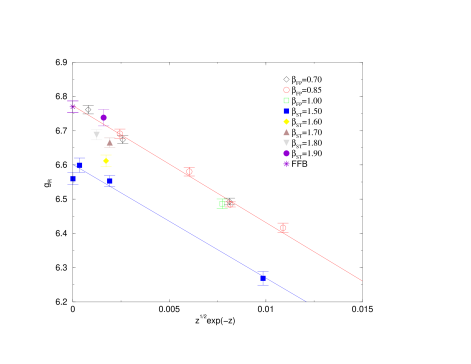
Figure 1: The coupling $g_{{\hbox{\sixrm R}}}(z,\beta)$ for the FP (open symbols) and standard actions (filled symbols) plotted vs. $\sqrt{z}\exp(-z)$. The correlation length for the FP action are in the range $3.2\ldots 12.2$ while for the standard action in $11\ldots 122$. The theoretical value from the FFB is also shown. The linear fits are motivated by the the $1/n$ prediction (3.43) and are based on the $\beta_{\rm ST}=1.50$ and $\beta_{\rm FP}=0.85$ data, respectively.

Figure 2: The measured values for $g_{{\hbox{\sixrm R}}}$ together with the corrected ones at $L/\xi=7.25$ for the standard action. The solid and dotted lines correspond to the fits (3.45) and (3.46) respectively.

Figure 3: The measured values of the $\chi/\xi^{2}$ ratio divided by the 4-loop approximation to the prediction (3.50).

Finally, we used (3.43) again to extrapolate the continuum result for the finite physical size $z=7.25$ to the thermodynamic limit $z=\infty$. Thus our final result based on the standard action lattice measurements is:

$$g_{{\hbox{\sixrm R}}}^{{\rm ST}}=6.77(2)\,.$$ (3.47)

This error contains both the ambiguity in using the fits (3.45) or (3.46) and the error in $a_{1}$.

$\beta$	$L$	runsxx	$L/\xi$xx	$\xi$xxx	$\chi$xxxx	$g_{{\hbox{\sixrm R}}}$xxx
1.5	$60$	110$\times$20k	5.469(10)	10.97(2)	173.76(31)	6.269(20)
1.5	$80$	344$\times$20k	7.253(7)	11.03(1)	175.95(11)	6.553(16)
1.5	$100$	350$\times$20k	9.050(8)	11.05(1)	176.51(6)	6.613(17)
1.5	$140$	361$\times$20k	12.68(1)	11.04(1)	176.30(5)	6.560(18)
1.6	$140$	214$\times$20k	7.361(15)	19.02(4)	447.30(6)	6.612(17)
1.7	$250$	367$\times$20k	7.246(4)	34.50(2)	1267.20(57)	6.665(14)
1.8	$500$	361$\times$20k	7.717(4)	64.79(3)	3839.07(1.54)	6.688(15)
1.9	$910$	101$\times$20k	7.4395(6)	122.32(1)	11884.9(7.0)	6.738(24)
1.95	$1230$	12$\times$20k	7.352(20)	167.30(45)	20835 (57)	6.751(78)
2.0	$1600$	4$\times$20k	6.949(25)	230.26(83)	36826(142)	6.981(132)
2.05	$2100$	5$\times$20k	6.804(67)	308.63(3.06)	63011(731)	6.608(216)

Table 3: $\xi$, $\chi=3G(0)$ and $g_{{\hbox{\sixrm R}}}$ for the standard action

The data for the FP action seem to lie on a universal curve (the slope of which roughly corresponds to the $1/n$ prediction) in spite of the extremely short correlation length. We interpret this as an indication that the lattice artifacts for the FP action are small, in any case smaller than our error bars. The measured values for the standard action show a considerable lattice artifact but the data at $z\approx 7$ seem to converge to the FP result with increasing $\xi$. Extrapolating the FS effects to $z=\infty$ we get

$$g_{{\hbox{\sixrm R}}}^{{\rm FP}}=6.77(2)$$ (3.48)

and $a_{1}=5.0(3)$. This extrapolation is based on the four $\beta_{\rm FP}=0.85$ data points but including all points of table 4 does not alter the extrapolation significantly.

Our results (3.47) and (3.48) are clearly above the value determined previously via finite size scaling [?], although statistically compatible with Kim’s error estimate. They are above the central values quoted on the basis of high temperature expansions discussed above but very consistent with each other and the result eq.(2.35) from the form factor bootstrap.

We would like to end this section with a comparison of an analytic prediction of the ratio $\chi/\xi^{2}$ with the MC data. In ref. [?] the perturbative short distance expansion of the spin 2-point function was refined to

$$S^{a_{1}a_{2}}(x,0)={Z\delta^{a_{1}a_{2}}\over 3\pi^{3}}\Big{(}\ln M|x|\Big{)}^{2}\Bigg{\{}1+O\Bigg{(}{\ln|\ln M|x||\over\ln M|x|}\Bigg{)}\Bigg{\}}\,.$$ (3.49)

The new result was the exact (though non-rigorous) determination of the overall nonperturbative constant. Using this we can straightforwardly derive the relation [?]

$${\chi\over\xi^{2}}={3\pi\gamma_{2}^{2}\over 4\delta_{2}}\,{1\over\beta^{2}}\,\Bigg{\{}1+\sum_{n=1}^{\infty}\,{c_{n}\over\beta^{n}}\Bigg{\}}\,.$$ (3.50)

The first three non-universal perturbative coefficients are known for the standard action lattice regularization [?]:

$$c_{1}=0.1816\,,\,\,\,c_{2}=0.1330\,,\,\,\,c_{3}=0.1362\,.$$ (3.51)

Fig. 3 shows the measured values of the $\chi/\xi^{2}$ ratio divided by the 4-loop approximation to the prediction (3.50). Note that (3.50) seems to be satisfied by our data to a better accuracy than the analogous one for $\xi$ alone [?], but the ratios decrease rapidly and we do not know if they eventually overshoot the asymptotic value of 1. Note also that the prediction (3.50) is independent of the $M/\Lambda_{{\rm\overline{MS\kern-0.35002pt}\kern 0.35002pt}}$ ratio $8/{\rm e}$ of ref. [?].

$\beta$	$L$	runs	$L/\xi$	0000$\xi$	$\chi$	$g_{{\hbox{\sixrm R}}}$
0.70	18	115$\times$360k	5.682(3)	3.168(1)	19.501(8)	6.493(10)
0.70	22	197$\times$360k	6.924(3)	3.177(1)	19.646(6)	6.674(12)
0.70	26	363$\times$360k	8.176(3)	3.180(1)	19.686(4)	6.761(12)
0.85	32	31$\times$600k	5.359(5)	5.971(5)	55.74(5)	6.417(14)
0.85	34	189$\times$360k	5.678(2)	5.988(2)	56.03(2)	6.485(8)
0.85	36	52$\times$360k	6.006(4)	5.994(4)	56.24(3)	6.581(13)
0.85	42	140$\times$360k	6.986(3)	6.012(3)	56.51(2)	6.691(14)
1.00	70	691$\times$100k	5.734(4)	12.207(8)0	189.4(1)	6.487(14)

Table 4: Data for the FP action.

4 Phase shift analysis from 4-spin correlators

The prediction for the scattering amplitude of two particles at center of mass momentum $p=M\sinh\frac{1}{2}\theta$ in the O(3) non-linear sigma model by Zamolodchikov and Zamolodchikov [?] is given by

$$S_{a^{\prime}b^{\prime};ab}(\theta)=\sum_{I=0}^{2}e^{2i\delta_{I}(p)}P^{I}_{a^{\prime}b^{\prime};ab}\,,$$ (4.52)

where $P^{I}$ are the isospin projectors and the phase shifts $\delta_{I}$ are given simply by

$$e^{2i\delta_{0}(p)}={\theta+2i\pi\over\theta-2i\pi}\,,$$ (4.53)

$$e^{2i\delta_{1}(p)}={\theta+2i\pi\over\theta-2i\pi}\,\cdot\,{\theta-i\pi\over\theta+i\pi}\,,$$ (4.54)

$$e^{2i\delta_{2}(p)}={\theta-i\pi\over\theta+i\pi}\,.$$ (4.55)

lattice	$\beta$	$T\times L$	$m^{-1}$	$mL$
A	1.54	$256\times 128$	13.632(6)	9.4
B	1.40	$128\times 64$	6.883(3)	9.3
D	0.85	$128\times 64$	6.03(1)	10.0
E	0.70	$64\times 32$	3.186(15)	10.6

Table 5: Parameters of simulations in the O(3) model. On lattices A, B the standard action was used while D and E denote simulations with the FP action.

$I$	$k$	$\delta_{\rm exact}$	$\delta_{\rm E}$	$\delta_{\rm WF}$	$t_{0}$	$M$	$\delta_{\rm LW}$
0	1	1.4595	1.36(3)	1.49(2)	1	20	1.36(7)
			1.45(5)	1.50(4)	8	8
	2	1.2840	1.25(2)	1.30(2)	1	20	1.22(3)
			1.38(6)	1.34(5)	8	8
1	1	0.1751	0.10(1)	0.17(3)	1	20	0.15(1)
			0.19(3)	0.19(5)	8	8
	2	0.2692	0.15(2)	0.23(2)	1	20	0.23(1)
			0.23(4)	0.24(5)	8	8
2	1	$-1.3874$	$-1.51(2)$	$-1.37(1)$	1	20	$-1.39(2)$
			$-1.43(3)$	$-1.36(2)$	8	8
	2	$-1.0944$	$-1.11(1)$	$-1.06(1)$	1	20	$-1.05(1)$
			$-1.04(2)$	$-1.06(2)$	8	8

Table 6: Phase shifts from lattice A

$I$	$k$	$\delta_{\rm exact}$	$\delta_{\rm E}$	$\delta_{\rm WF}$	$t_{0}$	$M$	$\delta_{\rm LW}$
0	1	1.4584	1.41(1)	1.48(1)	1	20	1.51(7)
			1.47(1)	1.49(1)	3	10
	2	1.2818	1.29(1)	1.29(1)	1	20	1.2(1)
			1.35(1)	1.30(1)	3	10
1	1	0.1764	0.09(1)	0.12(1)	1	20	0.14(1)
			0.12(1)	0.12(1)	3	10
2	1	$-1.3859$	$-1.42(1)$	$-1.35(1)$	1	20	$-1.38(2)$
			$-1.36(1)$	$-1.35(1)$	3	10
	2	$-1.0914$	$-1.05(1)$	$-1.03(1)$	1	20	$-1.02(1)$
			$-1.02(1)$	$-1.03(1)$	3	10
	3	$-0.9102$	$-0.78(2)$	$-0.78(1)$	1	20	$-0.81(2)$
			$-0.76(1)$	$-0.78(1)$	3	10

Table 7: Phase shifts from lattice B

$I$	$k$	$\delta_{\rm exact}$	$\delta_{\rm E}$	$\delta_{\rm WF}$
0	1	1.4726	1.47(3)	1.46(1)
	2	1.3107	1.29(2)	1.29(2)
1	1	0.1598	0.16(1)	0.14(2)
	2	0.2545	0.23(2)	0.27(1)
2	1	$-1.4056$	$-1.41(2)$	$-1.41(1)$
	2	$-1.1321$	$-1.15(1)$	$-1.16(1)$

Table 8: Phase shifts from lattice D.

$I$	$k$	$\delta_{\rm exact}$	$\delta_{\rm E}$	$\delta_{\rm WF}$
0	1	1.4664	1.49(1)	1.48(1)
	2	1.2977	1.27(1)	1.28(1)
1	1	0.1674	0.18(1)	0.15(1)
	2	0.2619	0.26(1)	0.28(1)
2	1	$-1.3968$	$-1.35(1)$	$-1.39(1)$
	2	$-1.1138$	$-1.14(1)$	$-1.13(1)$

Table 9: Phase shifts from lattice E.

Figure 4: The phase shifts in units of $\pi/2$ vs. $p/M$. The open symbols are from ref. [?]. The corresponding filled symbols are our measurements on the same lattices A and B, with the method discussed here. The crosses denote results using the FP action (D and E). The continuous curve corresponds to the ZZ S-matrix.

In fact the Zamolodchikovs specified the S-matrix for general $n\geq 3$ and these expressions have been verified to O$(1/n^{2})$ in the $1/n$-expansion. For the particular case of O(3), Lüscher and Wolff [?] checked the expressions for low energies using MC simulation. The agreement was completely satisfactory; in particular the data were consistent with the highly non-trivial non-perturbative property that the S-matrix at zero energy is repulsive $S_{a^{\prime}b^{\prime};ab}(0)=-\delta_{a^{\prime}b}\delta_{b^{\prime}a}$, which is a crucial condition in the FFB construction. We repeated the measurements of [?] for the standard action using a modified method of analysis. In addition we also performed measurements using the FP action. Since the S-matrix is the essential ingredient in the FFB construction we report the results here.

The method of Lüscher and Wolff [?] is based on the following idea: The momentum of one of the particles in a 2-particle state with zero total momentum in a periodic box (in 1-dimension) takes discrete values $p_{n}$ given by the periodicity condition

$$p_{n}L+2\delta(p_{n})=2\pi n\,.$$ (4.56)

Accordingly, the energy of this state is given by

$$E_{n}=2E^{(1)}(p_{n})=2\sqrt{p_{n}^{2}+M^{2}}\,,$$ (4.57)

where $E^{(1)}(p)$ is the energy of a 1-particle state with momentum $p$. From the measurement of the energy spectrum $E_{n}$ for some low lying states one can then calculate the momentum $p_{n}$ and using eq. (4.56) the phase shift $\delta(p_{n})$. Varying $L$ and taking different values of $n$ one can determine $\delta(p)$ at several values of its argument.

To determine the 2-particle energies the correlation matrix has been measured

$$C_{xy}(t)=\langle{\rm vac}|O(x,0)O(y,t)|{\rm vac}\rangle_{\rm c}\,,$$ (4.58)

where

$$O(x,t)=\frac{1}{L}\sum_{z=0}^{L-1}\sigma(z,t)\sigma(z+x,t)\,.$$ (4.59)

We omit here the $O(n)$ structure and indices. The subscript c in eq. (4.58) means that in the $I=0$ channel the vacuum contribution is subtracted.

Using the eigenvectors $|n\rangle$ of the transfer matrix as intermediate states one has

$$C_{xy}(t)=\sum_{n}{\rm e}^{-E_{n}t}\psi_{n}(x)\psi_{n}(y)\,,$$ (4.60)

where

$$\psi_{n}(x)=\langle{\rm vac}|O(x,0)|n\rangle$$ (4.61)

is the “wave function” of the corresponding state. The lowest energy states in eq. (4.60) are the 2-particle states and they will dominate at sufficiently large values of $t$.

Note that the relative momentum $2p_{n}$ of the 2-particle states is encoded not only in the energy $E_{n}$ but also in the wave function $\psi_{n}(x)$. For the symmetric wave functions ($I=0,2$ channels) one should have

$$\psi_{n}(x)=A\cdot\cos p_{n}(x-L/2),\text{ for }R<x<L-R\,,$$ (4.62)

and similarly with $\sin p_{n}(x-L/2)$ for the $I=1$ channel. Here $R$ is the ‘interaction range’: for a relative distance $x>R$ the particles propagate (essentially) freely.

One expects that the additional information obtained from the wave function will provide a more precise determination of $p$ and hence of $\delta(p)$.

4.1 Determination of the energy spectrum and wave functions.

The rank $N$ of the matrix $C(t)$ in eq. (4.60) is $L/2$, $L/2-1$ and $L/2+1$ in the $I=0,1,2$ channels, respectively. We assume that for $t\geq t_{0}$ (with some $t_{0}$) no more than $N$ states contribute to $C_{xy}(t)$, in the sense that the total contribution of the states $n>N$ is much smaller than the statistical error $\delta C_{xy}(t)$.

Lüscher and Wolff [?] suggested to determine the energies of the 2-particle states from the generalized eigenvalue problem

$$C(t)v_{n}=\lambda_{n}(t,t_{0})C(t_{0})v_{n}\,.$$ (4.63)

The eigenvalues of eq. (4.63) are given exactly by

$$\lambda_{n}(t,t_{0})={\rm e}^{-E_{n}(t-t_{0})}\,,$$ (4.64)

provided the sum in eq. (4.60) is restricted to $N$ terms, $1\leq n\leq N$. It is also easy to show that (with an appropriate normalization of $v_{n}$):

$$\psi_{n}(x)=\sum_{y}C_{xy}(t_{0})v_{n}(y)\,.$$ (4.65)

Solving eq. (4.63) involves an inversion of $C(t_{0})$, and the distortion of its small eigenvalues by the statistical noise is enhanced. This could affect strongly the values and the errors of $E_{n}$ obtained. For $t_{0}>1$ taking all $N\sim L/2$ states introduces significant instability in the result. Because of this, we have introduced a modification: before considering the generalized eigenvalue problem, we truncate the correlation function to an $M$-dimensional subspace ($M<N$) spanned by the first $M$ eigenvectors of $C(t_{0})$ (to those with the largest $M$ eigenvalues and still stable against the statistical fluctuations). The generalized eigenvalue problem, eq. (4.63) is written then for the matrices $\overline{C}(t)$ in this reduced basis. The energies we used were obtained from eqs. (4.63,4.64). We also determined $v_{n}(x)$ from eq. (4.63). One can use them as some given (nearly optimal) projectors which satisfy

$$\left(v_{m},C(t)v_{n}\right)=\delta_{mn}{\rm e}^{-E_{n}(t-t_{0})}\,.$$ (4.66)

Note that due to statistical errors in $C_{xy}(t)$ the obtained $v_{n}(x)$’s will differ from the true ones hence this equations will be only approximately valid. They provide a useful consistency check, and also a somewhat different method to determine $E_{n}$.

As an alternative way to get the phase shifts we used the momenta $p_{n}$ determined from the wave function using eq. (4.65). For a given $t_{0}$ and $M$ one can also check the self consistency of the obtained parameters by comparing $C_{xy}(t)$ built from $E_{n}$ and $\psi_{n}(x)$ (cf. eqs. (4.64,4.65)) with the MC result.

4.2 The results

We performed the calculations with the standard action for the same lattices (A,B) as in Ref. [?] . In addition, we also repeated the calculations using the fixed point action (FP) for the O(3) model [?,?]. The parameters of our measurements are summarized in Table 5 (here $m$ is the inverse of the exponential correlation length).

The phase shifts obtained from the analysis for the standard and FP actions are shown in fig. 4 together with the results from ref. [?]. The results for the standard action are also given in tables 6 and 7 and for the FP action in tables 8 and 9. The column $\delta_{\rm E}$ gives the phase shift calculated from the energy by eq. (4.63), WF labels the results obtained from the wave function, eq. (4.65). The data shown correspond to $t_{0}=3$, $M=10$ for lattice D, and $t_{0}=1$, $M=10$ for lattice E. However, the results – especially for $\delta_{\rm WF}$ – are quite stable against this choice. We took $R\sim 3/m$ in eq. (4.62). Taking into account that the correlation lengths used with the FP action were only $\xi\approx 3$ and $6$, the agreement with the analytic prediction is very good. Note, however, that similar suppression of lattice artifacts has been observed previously with this action for other observables [?,?,?].

Acknowledgements

We would like to thank Michael Karowski for useful discussions, and Paolo Butera, Paolo Rossi and Ettore Vicari for informative correspondence.

This investigation was supported in part by the Hungarian National Science Fund (OTKA) (under T016233 and T019917), and also by the Schweizerischer Nationalfonds. The work of M.N. was supported by NSF grant 97-22097.

References

-
[1]
K. Symanzik, Nucl. Phys. B226 (1983) 187
For a review see M. Lüscher, ”Improved Lattice Gauge Theories”, in Les Houches 1984, Proceedings, Critical Phenomena, Random Systems, Gauge Theories, 359-374; and ”Advanced Lattice QCD”, talk given at Les Houches Summer School in Theoretical Physics 1997, hep-lat/9802029 - [2] A. Patrascioiu and E. Seiler, Phys. Rev. Lett. 74 (1995) 1920
- [3] M. Lüscher, Nucl. Phys. B135 (1978) 1
- [4] A. B. and Al. B. Zamolodchikov, Ann. Phys. 120 (1979) 253; Nucl. Phys. B133 (1978) 525
- [5] F.A. Smirnov, ‘Form factors in Completely Integrable Models of Quantum Field Theory’, World Scientific, 1992
- [6] M. Karowski, in Field theoretical methods in particle physics, 1980, ed. W. Rühl, Pg. 307
- [7] M. Karowski and P. Weisz, Nucl. Phys. B139 (1978) 455
- [8] J. Balog, M. Niedermaier and T. Hauer, Phys. Lett. B386 (1996) 224
- [9] J. Balog and M. Niedermaier, Nucl. Phys. B500 (1997) 421; Phys. Rev. Lett. 78 (1997) 4151
- [10] H. Babujian, A. Fring, M. Karowski and A. Zapletal, Nucl. Phys. B538 (1999) 535
- [11] M. Lüscher und U. Wolff, Nucl. Phys. B339 (1990) 222
- [12] J. Balog, M. Niedermaier, F. Niedermayer, A. Patrascioiu, E. Seiler and P. Weisz, in preparation
- [13] P. Hasenfratz and F. Niedermayer, Nucl. Phys. B414 (1994) 785
- [14] P. Hasenfratz, M. Maggiore and F. Niedermayer, Phys. Lett. B245 (1990) 522
- [15] A. Patrascioiu and E. Seiler, Phys. Letts. B445 (1998) 160
- [16] A. Pelissetto and E. Vicari, Nucl. Phys. B519 (1998) 626
- [17] M. Falcioni, G. Martinelli, M. L. Paciello, G. Parisi and B. Taglienti, Nucl. Phys. B225 (1983) 313
- [18] P. Butera and M. Comi, Phys. Rev. B54 (1996) 15828; ibid B50 (1994) 3052; ibid B58 (1998) 11552
- [19] M. Campostrini, A. Pelissetto, P. Rossi and E. Vicari, Phys. Letts. B402 (1997) 141
- [20] M. Campostrini, A. Pelissetto, P. Rossi and E. Vicari, Nucl. Phys. B459 (1996) 207; Nucl. Phys. Proc. Suppl. 47 (1996) 751
- [21] P. Rossi and E. Vicari, private communication
- [22] M. Campostrini, A. Pelissetto, P. Rossi and E. Vicari, Phys. Rev. B54 (1996) 7301
- [23] M. Campostrini, A. Pelissetto, P. Rossi and E. Vicari, Phys. Phys. D54 (1996) 1782; Nucl. Phys. Proc. Suppl. 47 (1996) 755
- [24] J. Balog, M. Niedermaier, F. Niedermayer, A. Patrascioiu, E. Seiler and P. Weisz, in preparation
- [25] P. Butera, private communication
- [26] J. Kim, Phys. Lett. B345 (1995) 469
- [27] S. Caracciolo and A. Pelissetto, Nucl. Phys. B455 (1995) 619
- [28] C. Michael, Nucl. Phys. B259 (1985) 58
- [29] M. Blatter, R. Burkhalter, P. Hasenfratz and F. Niedermayer, Phys. Rev. D53 (1996) 923
- [30] S. P. Spiegel, Phys. Lett. B400 (1997) 352