BI-TP 99/04
hep-lat/9903030
March 1999
revised version

The quenched limit of lattice QCD
at non-zero baryon number

J. Engels, O. Kaczmarek, F. Karsch and E. Laermann

Fakultät für Physik, Universität Bielefeld, D-33615 Bielefeld, Germany

ABSTRACT

We discuss the thermodynamics of gluons in the background of static quark sources. In order to do so we formulate the quenched limit of QCD at non-zero baryon number. A first numerical analysis of this system shows that it undergoes a smooth deconfining transition. We find evidence for a region of coexisting phases that becomes broader with increasing baryon number density. Although the action is in our formulation explicitly $Z(3)$ symmetric the Polyakov loop expectation value becomes non-zero already in the low temperature phase. It indicates that the heavy quark potential stays finite at large distances, i.e. the string between static quarks breaks at non-zero baryon number density already in the hadronic phase.

PACS-Indices: 5.70.Ce  12.38.Gc  11.30.F

Keywords: Finite baryon density, Non-zero baryon number,

Deconfinement transition, Quenched limit

1 Introduction

Numerical studies of the $SU(3)$ gauge theory, i.e.  the heavy quark mass (quenched) limit of QCD, are extremely helpful for the understanding of the phase structure of QCD at non-zero temperature. The deconfining phase transition as well as basic properties of the low and high temperature phases can be studied in this approximation, although the phase transition in the light quark mass (chiral) limit differs not only on a quantitative level but also qualitatively; in the chiral limit the order of the transition is controlled by the chiral symmetry of the fermionic part of the QCD Lagrangian whereas in the quenched limit the $Z(3)$ center symmetry dictates the order of the transition. Nonetheless, the fundamental features of deconfinement which are reflected, for instance, in the release of many new degrees of freedom at $T_{c}$, are similar in both limits. This leads to a quite similar temperature dependence of bulk thermodynamic observables like the pressure and energy density [1].

So far the investigations of QCD thermodynamics were essentially limited to the case of vanishing baryon number. In the case of non-zero baryon number, usually realized in thermodynamic calculations through the introduction of a non-zero chemical potential ($\mu$) [2, 3], little is known from lattice calculations about the behaviour of thermodynamic observables, the QCD phase diagram and the properties of the different phases. The reason for this is well-known. The probabilistic interpretation of the path integral representation of the QCD partition function breaks down as soon as one introduces a non-zero chemical potential. Moreover, even the naive quenched limit at non-zero chemical potential, i.e. the ordinary $SU(3)$ gauge theory at $\mu=0$, turned out to be pathological when fermionic observables with $\mu\neq 0$ are analyzed [4]. In fact, it is understood that this naive limit is not the correct quenched limit of finite density QCD; it is the zero flavour limit of a theory with equal number of fermion flavours carrying baryon number $B$ and $-B$, respectively. [5].

As the relativistic chemical potential $\mu$ also contains a contribution proportional to the rest mass of the quarks, the static limit of QCD at non-zero chemical potential requires to take a double limit in which the quark mass as well as the chemical potential is taken to infinity while an appropriate ratio is kept fixed. This limit has been formulated in [6, 7]. It seems that in this case the first order deconfining phase transition of the $SU(3)$ gauge theory turns into a crossover for arbitrarily small, non-zero values of the chemical potential [7]. However, although at non-zero chemical potential the thermal phase transition may get lost as a true singularity of the partition function of quenched QCD, we still expect the quenched theory to resemble the physics of deconfinement – gluon thermodynamics in the background of a non-zero number of static quark sources is expected to lead to deconfinement at high temperature. It is then interesting to analyze the nature of this transition and study in how far static quark sources in a gluonic heat bath influence the deconfinement of gluons and, for instance, the heavy quark potential. We will discuss here a framework for the analysis of these questions – quenched QCD at fixed baryon number – and will present first numerical simulations which address these questions.

Rather than introducing a non-vanishing chemical potential, i.e. formulate QCD at non-vanishing baryon number density in the grand canonical ensemble, one may go over to a canonical formulation of the thermodynamics and fix directly the baryon number [10]. This is achieved by introducing an imaginary chemical potential [10, 11] in the grand canonical partition function. Performing subsequently a Fourier integration allows to project onto the canonical partition function for a given sector of fixed baryon number [10]. In the heavy quark mass limit one is then left with a well-defined quenched theory at fixed baryon number – gluon thermodynamics in the background of a non-zero number of static quark sources, suitably arranged to obey Fermi statistics.

Despite the fact that the grand canonical formulation of finite density QCD leads to severe numerical problems [12] the alternative canonical approach at non-zero baryon number so far did find only little attention. To some extent this may be justified. Introducing a constraint on the total number of fermions (quarks minus anti-quarks) in general leads to rather complicated non-local constraints for the gauge field sector. However, in view of the problems that arise in the standard non-zero chemical potential formulation and that grow exponentially with the size of the volume one may seriously want to analyze also the canonical approach in more detail. We will show here that the formulation of QCD at non-zero baryon number does have a well defined, non-trivial heavy quark mass (quenched) limit which can be analyzed numerically at least for moderate baryon number densities.

In the grand canonical formulation the Fermion determinant becomes complex for any non-zero chemical potential leading to all the conceptual and algorithmic problems. In the canonical approach, on the other hand, the determinant stays real. However, as should be obvious, the problems related to a non-positive integration measure are not solved that easily. The Fourier transformation which is needed in the canonical formulation to project onto the sector with fixed baryon number reintroduces negative contributions to the partition function and one thus again faces algorithmic problems. Performing the Fourier integration numerically thus seems to be ruled out; one can, however, do it explicitly. This leads to a complicated expression in terms of products of quark propagators which may be viewed as the boundary conditions for the gauge fields needed to project onto a sector with fixed baryon number. We will use this as a starting point for our analysis of the heavy quark mass, quenched, limit.

In the next section we will discuss the canonical formulation of QCD at finite baryon number and, in particular, introduce the quenched limit. In section 3 we will present some results of a first numerical analysis of this quenched theory. Section 4 contains our conclusions. In an appendix we give explicit representations for the canonical partition function for some values of the baryon number.

2 Lattice  formulation  of  QCD  with  non-zero baryon number

The general framework for going from a grand canonical formulation of QCD at non-zero baryon number density in terms of a non-vanishing chemical potential [2, 3] to a canonical formulation with a fixed baryon number has been outlined in [10]. As mentioned before the main difficulty of this approach arises from the need to perform a Fourier transformation to eliminate the chemical potential in favour of a fixed baryon number. We will show in the following that this integration can be performed explicitly. The projection onto a given sector of fixed baryon number is then contained in a rather complicated sum over products of quark propagators. This representation probably is too complicated to be useful for numerical calculations with arbitrary, e.g. the physically interesting, light quark masses. However, it may provide a new starting point for physically relevant approximations to the complete problem. In particular, we will discuss in the next section the quenched limit at fixed baryon number, i.e.  gluon thermodynamics in the background of static quarks.

Starting from the standard formulation of QCD at non-zero chemical potential [2] and the corresponding formulation at non-zero baryon number [10] we will rewrite the fermion sector of the lattice action in a somewhat more transparent form which makes clear that the non-vanishing chemical potential can be viewed as a modification of the temporal boundary conditions for the fermion fields. To be specific we will use the Wilson formulation of the fermion action. Although we will eventually restrict our discussion to the static limit, which also can be obtained directly from the heavy quark formulation for Wilson fermions derived in analogy to the approach given in Ref. [7] for staggered fermions, we will start here by formulating the canonical approach for arbitrary quark masses.

The action for Wilson fermions at non-zero chemical potential is given by

$$S_{F}(\mu a) \equiv \bar{\psi}Q\psi$$ (2.1)

$$= \sum_{x}\biggl{(}\bar{\psi}_{x}\psi_{x}-\kappa\sum_{j=1}^{3}\bigl{[}\bar{\psi}_{x}(1-\gamma_{j})U_{x,j}\psi_{x+\hat{j}}+\bar{\psi}_{x+\hat{j}}(1+\gamma_{j})U_{x,j}^{\dagger}\psi_{x}\bigr{]}$$

$$-\kappa\bigl{[}{\rm e}^{\mu a}\bar{\psi}_{x}(1-\gamma_{4})U_{x,4}\psi_{x+\hat{4}}+{\rm e}^{-\mu a}\bar{\psi}_{x+\hat{4}}(1+\gamma_{4})U_{x,4}^{\dagger}\psi_{x}\bigr{]}\biggr{)}~{}~{}.$$

Here $\kappa$ is the hopping parameter which controls the value of the quark mass, $x=(\vec{x},x_{4})$ denotes the sites on a lattice of size $N_{\sigma}^{3}\times N_{\tau}$. The Grassmann fields obey anti-periodic boundary conditions in the time direction (fourth direction), i.e.  $\psi_{(\vec{x},N_{\tau}+1)}=-\psi_{(\vec{x},1)}$ and $\bar{\psi}_{(\vec{x},N_{\tau}+1)}=-\bar{\psi}_{(\vec{x},1)}$.

We may shift the dependence on the chemical potential to the last time slice, which connects the hyperplanes with $x_{4}=N_{\tau}$ and $x_{4}=1$, by transforming the fermion fields

$$\psi_{(\vec{x},x_{4})}^{\prime}={\rm e}^{\mu ax_{4}}\psi_{(\vec{x},x_{4})}\quad,\quad\bar{\psi}_{(\vec{x},x_{4})}^{\prime}={\rm e}^{-\mu ax_{4}}\bar{\psi}_{(\vec{x},x_{4})}\qquad.$$ (2.2)

This eliminates the dependence on the chemical potential on all time slices but the last one, which now reads

$$S_{F}^{N_{\tau}}(\mu/T)=\kappa\sum_{\vec{x}}\bigl{[}{\rm e}^{\mu/T}\bar{\psi}_{(\vec{x},N_{\tau})}(1-\gamma_{4})U_{x,4}\psi_{(\vec{x},1)}+{\rm e}^{-\mu/T}\bar{\psi}_{(\vec{x},1)}(1+\gamma_{4})U_{x,4}^{\dagger}\psi_{(\vec{x},N_{\tau})}\bigr{]}~{},$$ (2.3)

with $x\equiv(\vec{x},N_{\tau})$. We also have used the definition of the temperature $1/T=aN_{\tau}$ in writing $\mu/T=\mu aN_{\tau}$ and furthermore explicitly took care of the anti-periodic boundary conditions for the fermions. The remaining part of the fermion action, which now is independent of the chemical potential, may be written as

$$\tilde{S}_{F}=S_{F}(0)-S_{F}^{N_{\tau}}(0)\quad.$$ (2.4)

This representation explicitly shows that the formulation of thermodynamics with non-zero chemical potential can be viewed as a generalization of the non-zero temperature case, which is realized through anti-periodic boundary conditions in the fermion sector. They are now generalized to $\psi_{(\vec{x},N_{\tau}+1)}=-\exp{(\mu/T)}~{}\psi_{(\vec{x},1)}$ and $\bar{\psi}_{(\vec{x},N_{\tau}+1)}=-\exp{(-\mu/T)}~{}\bar{\psi}_{(\vec{x},1)}$.

So far we have only re-organized the various terms in the fermion sector of the QCD partition function where we have used the standard Wilson formulation. For the gluon sector we do not have to specify at this point the explicit form of the action, $S_{G}$. The partition function in a volume $V=(N_{\sigma}a)^{3}$ at temperature $T=1/N_{\tau}a$ and non-zero chemical potential $\mu a$ then reads,

$$Z(\mu/T,T,V)=\int\prod_{x,\nu}{\rm d}U_{x,\nu}\prod_{x}{\rm d}\bar{\psi}_{x}{\rm d}\psi_{x}{\rm e}^{-S_{F}^{N_{\tau}}(\mu/T)}{\rm e}^{-S_{G}-\tilde{S}_{F}}~{}~{}.$$ (2.5)

We want to use this form as a starting point to go over to a formulation at non-zero baryon number rather than at non-zero chemical potential. This can be achieved by introducing a complex chemical potential and performing a Fourier transformation,

$$Z(B,T,V)={1\over 2\pi}\int_{0}^{2\pi}{\rm d}\phi\ {\rm e}^{-iB\phi}\ Z(i\phi,T,V)~{}~{},$$ (2.6)

where $B$ denotes the quark number, i.e. the baryon number equals $B/3$. The Fourier transformation only operates on the factor ${\rm e}^{-S_{F}^{N_{\tau}}}$ which only involves links pointing in the 4th direction on the last time slice of the lattice. Making use of the Grassmann properties of the fermion fields this contribution can be written as

$${\rm e}^{-S_{F}^{N_{\tau}}(i\phi)}=\prod_{(\vec{x},a,b,\alpha,\beta,f)} \biggl{(}1-\kappa{\rm e}^{i\phi}\bar{\psi}_{(\vec{x},N_{\tau})}^{a,\alpha,f}{\cal U}_{\vec{x}}^{a,\alpha,b,\beta}\psi_{(\vec{x},1)}^{b,\beta,f}\biggr{)}\times$$

$$\prod_{(\vec{x},a,b,\alpha,\beta,f)} \biggl{(}1-\kappa{\rm e}^{-i\phi}\bar{\psi}_{(\vec{x},1)}^{a,\alpha,f}{\cal U}_{\vec{x}}^{\dagger a,\alpha,b,\beta}\psi_{(\vec{x},N_{\tau})}^{b,\beta,f}\biggr{)}~{},$$ (2.7)

where the product runs over all possible combinations of indices with $\vec{x}$ taking values on the three dimensional (spatial) lattice of size $N_{\sigma}^{3}$. We also have introduced the notation ${\cal U}_{\vec{x}}=\Gamma_{-}U_{(\vec{x},N_{\tau}),4}$ and ${\cal U^{\dagger}}_{\vec{x}}=\Gamma_{+}U_{(\vec{x},N_{\tau}),4}^{\dagger}$ with $\Gamma_{\pm}=(1\pm\gamma_{4})$. Note that the fields ${\cal U}$ carry spinor and color indices which we denote by Greek and Latin letters, respectively. We will combine these to a single index denoted by, e.g. ${\cal A}=(\alpha,a)$ with $\alpha=1,...,4$ and $a=1,~{}2,~{}3$. In addition we also have allowed for different fermion flavours, $f=1,...,n_{f}$ but ignored the possibility of having different quark masses, i.e. different hopping parameters $\kappa$ for the various flavours.

We may expand the product appearing in Eq. 2.7 and write it as a series in terms of the complex fugacity, $z=\exp(i\phi)$. The Fourier transformation in Eq. 2.6 will receive a non-zero contribution only from the term proportional to $z^{B}$. The coefficient of $z^{B}$ will receive contributions from $n$ terms proportional to $z$ and $\bar{n}$ terms proportional to $z^{*}$ where $B=n-\bar{n}$. Each such contribution is proportional to $\kappa^{n+\bar{n}}$. This is the basis for a systematic hopping parameter expansion for the boundary term. Clearly we need at least $B$ terms proportional to $z$. The leading contribution thus arises from the $\bar{n}\equiv 0$ sector. It can be summarized as

$$z^{B}f_{B}\equiv(-z\kappa)^{B}\sum_{X,{\cal C,D},F}\prod_{i=1}^{B}\bar{\psi}_{(\vec{x}_{i},N_{\tau})}^{{\cal C}_{i},f_{i}}{\cal U}_{\vec{x}_{i}}^{{\cal C}_{i},{\cal D}_{i}}\psi_{(\vec{x}_{i},1)}^{{\cal D}_{i},f_{i}}~{}~{},$$ (2.8)

where $X,~{}{\cal C,~{}D},~{}F$ are $B$-dimensional vectors, i.e.  $X=(\vec{x}_{1},...,\vec{x}_{B})$, $F=(f_{1},...,f_{B})$ and so on. Of course, all elements of the set of indices $\{({\cal C}_{i},f_{i},\vec{x}_{i})\}_{i=1}^{B}$ as well as $\{({\cal D}_{i},f_{i},\vec{x}_{i})\}_{i=1}^{B}$ have to be different to give a non-vanishing contribution to the sum in Eq. 2.8. The Fourier integral in Eq. 2.6 can then be performed explicitly and we obtain for the partition function at fixed baryon (or quark) number

$$Z(B,T,V)=\int\prod_{x,\nu}{\rm d}U_{x,\nu}\prod_{x}{\rm d}\bar{\psi}_{x}{\rm d}\psi_{x}f_{B}~{}{\rm e}^{-S_{G}-\tilde{S}_{F}}~{}~{}.$$ (2.9)

To leading order in the hopping parameter the projection onto a sector with fixed quark number $B$ is encoded in the function $f_{B}$ which is a sum over products of quark propagators between the time slices at $x_{4}=1$ and $x_{4}=N_{\tau}$. In higher orders one will, of course, also get contributions from quarks propagating backward in Euclidean time. In fact, if we think in terms of a hopping parameter expansion (heavy quark mass limit) for the entire fermion determinant, the function $f_{B}$ is all we need to generate the leading contribution, which finally will be ${\cal O}(\kappa^{BN_{\tau}})$. Higher order contributions will result from $\phi$-independent terms coming from an expansion of $\exp(-\tilde{S}_{F})$ as well as from additional factors in the expansion of Eq. 2.7 which then have to contain an equal number of additional backward and forward propagating terms.

Let us look in more detail at the leading contribution arising from $f_{B}$. For this it is convenient to evaluate $f_{B}$, which of course is a gauge invariant function, in a specific gauge. Let us perform a gauge transformation such that all the links pointing in the time direction on the last time slice are equal to unity. This gives

$$f_{B}=(-2\kappa)^{B}\sum_{X,{\cal A},F}\prod_{i=1}^{B}\bar{\psi}_{(\vec{x}_{i},N_{\tau})}^{{\cal A}_{i},f_{i}}\psi_{(\vec{x}_{i},1)}^{{\cal A}_{i},f_{i}}~{}~{}.$$ (2.10)

Like in Eq. 2.8 the vectors $X,~{}{\cal A},~{}F$ are of length $B$. However, now the spinor indices $\alpha_{i}$ which are part of ${\cal A}_{i}$ only take on the values $\alpha_{i}=1,~{}2$ because only the two components of $\Gamma_{-}$ are non-zero. This also gives rise to the factors of $2$ in front of $\kappa$. When evaluating the Grassmann integrals each of the $\bar{\psi}$ terms can be contracted with all those $\psi$ terms which carry the same flavour index. Each pair gives rise to a matrix element of the inverse of $\tilde{Q}$, the fermion matrix corresponding to $\tilde{S}_{F}$. The different pairings give rise to the Matthews-Salam determinant [15]. We thus will get the product of $n_{f}$ determinants, each of dimension $d_{l}$ such that $\sum_{l=1}^{n_{f}}d_{l}=B$,

$$\hat{f}_{B}=(2\kappa)^{B}\sum_{X,{\cal A},F}\prod_{l=1}^{n_{f}}{\rm det}{\cal M}_{l}[x,{\cal A}]~{}~{},$$ (2.11)

where the matrix ${\cal M}_{l}$ gives the contributions for the l-th flavour and the matrix elements are the corresponding quark propagators,

$${\cal M}_{l}^{i,j}=\tilde{Q}^{-1}_{((\vec{x}_{j},1),{\cal A}_{j}),((\vec{x}_{i},N_{\tau}),{\cal A}_{i})}~{}~{}.$$ (2.12)

Each matrix element of ${\cal M}_{l}$ is ${\cal O}(\kappa^{(N_{\tau}-1+|\vec{x}_{i}-\vec{x}_{j}|)})$. In the limit of small $\kappa$-values, i.e.  in the heavy quark mass limit, only matrix elements of ${\cal M}$ with $|\vec{x}_{i}-\vec{x}_{j}|=0$ will thus survive. In this case the elements of $\tilde{Q}^{-1}_{((\vec{x}_{i},1),{\cal A}_{j}),((\vec{x}_{i},N_{\tau}),{\cal A}_{i})}$ are just products of terms $\Gamma_{-}U_{(\vec{x}_{i},k),4}$ with $k=1,..,N_{\tau}-1$. As $\Gamma_{-}$ is a diagonal matrix in spinor space the indices $\alpha_{i}$ and $\alpha_{j}$ have to be identical. The spinor part thus gives rise to an overall factor $2^{N_{\tau}-1}$ for each $i$, i.e. we obtain $B$ such factors. The multiplication of the SU(3) matrices yields an element of the ordinary, complex valued (!) Polyakov loop ($U\equiv 1$ on the last time slice !) which we denote by $L_{\vec{x}_{i}}^{a_{i},a_{j}}$. Finally, the sum over different colour indices appearing in Eq. 2.11 leads to contributions involving only traces over powers of the Polyakov loop,

$$L_{\vec{x}}=\prod_{x_{4}=1}^{N_{\tau}}U_{(\vec{x},x_{4})}~{}~{}.$$ (2.13)

As the (colour, spinor) label ${\cal A}_{i}$ can take on six different values the determinant is non-zero only if at most six quarks of a given flavour occupy a given site $\vec{x}_{i}$. At most three quarks can have the same spinor component. There are thus six possible contributions, $D_{n}$, of a given site to the determinant depending on the quark occupation number, $n$, of this site. These can be expressed in terms of three functions $M_{i}$ which correspond to the number of quarks ($i$) with identical spinor components. These contributions are

$$D_{1} = 2M_{1}$$

$$D_{2} = 2(M_{1}^{2}+M_{2})$$

$$D_{3} = 2(3M_{1}M_{2}+M_{3})$$

$$D_{4} = 2(4M_{1}M_{3}+3M_{2}^{2})$$

$$D_{5} = 20M_{2}M_{3}$$

$$D_{6} = 20M_{3}^{2}\quad,$$ (2.14)

with

$$M_{1}={\rm Tr}L_{\vec{x}_{i}}\quad,\quad M_{2}=({\rm Tr}L_{\vec{x}_{i}})^{2}-{\rm Tr}L_{\vec{x}_{i}}^{2}\quad,\quad M_{3}=6\quad.$$ (2.15)

We note that this representation is quite similar to that of the heavy quark mass limit for QCD with staggered fermions at non-zero chemical potential [7].

We now may write $\hat{f}_{B}$ as

$$\hat{f}_{B} = (2\kappa)^{BN_{\tau}}\sum_{X,F}\prod_{k=1}^{B^{\prime}}\prod_{l=1}^{n_{f}}D_{n_{k,l}}(\vec{x}_{k})\quad,$$ (2.16)

where $B^{\prime}\leq B$ is the number of distinct sites $\vec{x}_{k}$ appearing in $X$ and $n_{k,l}$ is the occupation number for these distinct sites $\vec{x}_{k}$ with quarks of flavour $l$. They obey the constraint $\sum_{k,l}n_{k,l}=B$ with $0\leq n_{k,l}\leq 6$. The total number of quarks at the site $\vec{x}_{k}$ is $n_{k}=\sum_{l}n_{k,l}$. The sum over all different distributions of the flavour number can be performed locally for a given distribution of sites $X$. Let us define

$$\bar{D}_{n_{k}}(\vec{x}_{k})=\sum_{n_{k,1}=0}^{\bar{n}_{k}}...\sum_{n_{k,n_{f}}=0}^{\bar{n}_{k}}\delta(n_{k}-\sum_{l=1}^{n_{f}}n_{k,l})\prod_{l=1}^{n_{f}}D_{n_{k,l}}(\vec{x}_{k})\quad,$$ (2.17)

with $\bar{n}_{k}={\rm min}(n_{k},6)$. We then can write Eq. 2.16 as

$$\hat{f}_{B} = (2\kappa)^{BN_{\tau}}\sum_{X}\prod_{k=1}^{B^{\prime}}\bar{D}_{n_{k}}(\vec{x}_{k})\quad.$$ (2.18)

One of the difficulties with using a representation like Eq. 2.16 or Eq. 2.18 in a numerical calculation is that there appears a $B$-fold sum over the volume, $V$, with constraints on the occupation number for a given site, i.e. the computational effort would be ${\cal O}(V^{B})$. Through a cluster decomposition we can, however, reduce this to the evaluation of certain moments of $\bar{D}_{i}$ as well as their average on a given configuration. This is described in the Appendix.

We finally obtain

$$\hat{f}_{B} = (2\kappa)^{BN_{\tau}}\sum_{\{g_{\alpha}\}}\delta\biggr{(}B-\sum_{l=1}^{6n_{f}}\sum_{\{\alpha\}}lg_{\alpha}a_{l}\biggl{)}\times$$ (2.19)

$$\prod_{\{\alpha\}}{1\over g_{\alpha}!}\biggl{\{}(-1)^{(\sum_{l=1}^{6n_{f}}a_{l}-1)}\biggl{(}(\sum_{l=1}^{6n_{f}}a_{l}-1)!\biggl{[}\prod_{l=1}^{6n_{f}}{1\over a_{l}!}\bar{D}_{l}^{a_{l}}\biggr{]}\biggr{)}\biggr{\}}^{g_{\alpha}}\quad,$$

where $[...]$ is the mean value defined in (A.6) and the product runs over all possible sets of vectors $\alpha=(a_{1},...,a_{6n_{f}})$ which are constrained by

$$\sum_{l=1}^{6n_{f}}la_{l}\leq B\quad.$$ (2.20)

The sum over $g_{\alpha}$ is defined in (A.11).

Now we have achieved that only simple sums over products of suitably chosen terms $\bar{D}_{n}$ have to be evaluated to obtain the contribution $\hat{f}_{B}$ to the partition function which results from a given number of static quarks. The number of possible partitions contributing to Eq. 2.19 grows, however, rapidly with $B$. After all it is nothing else but the result of an explicit evaluation of the fermion determinant in a fixed baryon number sector. As $\hat{f}_{B}$ contains products of mean values calculated on a given configuration, it is a non-local quantity which in a Monte-Carlo simulation has to be evaluated for each update of a temporal link. In practice, calculations thus will be limited to small values of $B$. Some explicit representations of $\hat{f}_{B}$ for small values of $B$ are given in the appendix. In the next section we will use this representation of the quenched limit of the QCD partition function with fixed baryon number. We will perform first exploratory Monte-Carlo simulations to analyze the phase structure of gluon thermodynamics in the presence of static quarks.

3 Simulation  of  quenched  QCD  with  non-zero baryon number

For any fixed value of the baryon number we can write the quenched partition function as

$$Z(B,T,V)=\int\prod_{x,\nu}{\rm d}U_{x,\nu}~{}\hat{f}_{B}~{}{\rm e}^{-S_{G}}~{}~{},$$ (3.1)

where the constraint on the baryon number is encoded in the function $\hat{f}_{B}$ given in Eq. 2.16. In particular, we note that the global $Z(3)$ symmetry of the QCD partition function at non-zero baryon number is preserved also in the quenched limit, i.e. the function $\hat{f}_{B}$ is invariant under global $Z(3)$ transformations if $B$ is a multiple of $3$. As the gluonic action $S_{G}$ also shares this property the partition function, $Z(B,T,V)$, is non-zero only if $B$ is a multiple of $3$.

We also note that $\hat{f}_{B}$ is still a complex function. However, upon integration over the gauge fields the imaginary contribution vanishes; the partition function is real, of course. Actual calculations thus can be performed with ${\rm Re}\hat{f}_{B}$. The crucial question for a simulation with this partition function is whether the remaining sign changes of the real part of $\hat{f}_{B}$ are seldom enough so that a Monte-Carlo simulation can be performed with the absolute value of ${\rm Re}\hat{f}_{B}$ and the overall sign can be included in the calculation of averages [16].

We will perform simulations for the one flavour case $(n_{f}=1)$ using the partition function

$$Z_{||}(B,T,V)=\int\prod_{x,\nu}~{}{\rm d}U_{x,\nu}|{\rm Re}\hat{f}_{B}|~{}{\rm e}^{-S_{G}}~{}~{}.$$ (3.2)

Expectation values of an observable ${\cal O}$ calculated with the Boltzmann weights defined by the partition function $Z(B,T,V)$ will therefore be calculated according to

$$\langle{\cal O}\rangle={\langle{\cal O}\cdot{\rm sgn}({\rm Re}\hat{f}_{B})\rangle_{||}\over\langle{\rm sgn}({\rm Re}\hat{f}_{B})\rangle_{||}}~{}~{}.$$ (3.3)

Our simulations are performed on lattices of size $8^{3}\times 2$ and $10^{3}\times 2$ using the standard Wilson gauge action [17]. For the link updates we use a Metropolis algorithm. For each link update the change in the function ${\rm Re}\hat{f}_{B}$ is calculated and a possible change in sign is monitored. In all the cases we have studied so far we find that $\langle{\rm sgn}({\rm Re}\hat{f}_{B})\rangle_{||}$ is large and can be well determined. In fact, for large values of the temperature ${\rm sgn}({\rm Re}\hat{f}_{B})$ is almost always positive. This is evident from Figure 1 which shows the average sign as a function of the coupling $\beta$. The expectation value of ${\rm sgn}({\rm Re}\hat{f}_{B})$ mainly depends on the spatial volume $N_{\sigma}$ but varies little with $B$ at fixed $N_{\sigma}$. We also find that the values of observables like the average action or the Polyakov loop do not depend much on the sign of ${\rm Re}\hat{f}_{B}$ so that the errors obtained for these observables from a jackknife analysis are substantially smaller than those shown in Figure 1.

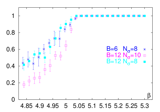
Figure 1: Expectation value of the sign of ${\rm Re}\hat{f}_{B}$, $\langle{\rm sgn(Re}\hat{f}_{B})\rangle_{||}$, for $B=6$ and 12 and lattices of size $N_{\sigma}^{3}\times 2$ with $N_{\sigma}=8$ and 10.

A numerical analysis of the thermodynamics at fixed baryon number, $B$, can closely follow the standard approach at $B=0$, i.e. in a pure $SU(3)$ gauge theory [19]. We may analyze the temperature dependence of bulk thermodynamics, the Polyakov loop expectation value and other observables for a gluon gas in the background of static quarks. We started a first exploratory analysis of this system by performing a numerical simulation on lattices with temporal extent $N_{\tau}=2$. The simulations have been carried out in the vicinity of the critical coupling for the deconfinement transition at $B=0$, i.e. for gauge couplings $\beta\simeq 5.0$ which are still in the strong coupling regime. Calculations with fixed $B$ are performed on lattices of size $N_{\sigma}^{3}\times N_{\tau}$ and the temperature is varied, as usual, by changing the coupling $\beta=6/g^{2}$. The dimensionless parameter kept fixed in the simulation thus is the baryon number density in units of the temperature cubed,

$${n_{B}\over T^{3}}={B\over 3}\biggl{(}{N_{\tau}\over N_{\sigma}}\biggr{)}^{3}~{}~{}.$$ (3.4)

The baryon number density in physical units thus is

$$n_{B}={B\over 3}\biggl{(}{N_{\tau}\over N_{\sigma}}\biggr{)}^{3}\biggl{(}{T\over 200~{}{\rm MeV}}\biggr{)}^{3}{\rm fm}^{-3}~{}~{}.$$ (3.5)

For orientation we note that close to $T_{c}$, which for the $SU(3)$ gauge theory is known to be about $270$ MeV, a simulation on an $8^{3}\times 2$ lattice with $B=12$ corresponds to $n_{B}\simeq 0.15/{\rm fm}^{3}$, i.e. approximately nuclear matter density.

For vanishing baryon number the Polyakov loop expectation value or more precisely the expectation value of its normalized absolute value calculated on a finite lattice,

$$\langle|L|\rangle_{V}=\langle\bigl{|}{1\over 3N_{\sigma}^{3}}\sum_{\vec{x}}{\rm Tr}L_{\vec{x}}\bigr{|}\rangle~{}~{},$$ (3.6)

is an order parameter for the deconfinement transition in the infinite volume limit,

$$\langle L\rangle\equiv\lim_{N_{\sigma}\rightarrow\infty}\langle|L|\rangle_{V}~{}~{}.$$ (3.7)

As the phase transition is first order in $SU(3)$, $\langle L\rangle$ changes discontinuously at $T_{c}$. Besides being related to the spontaneous breaking of the global $Z(3)$ symmetry of the pure gauge action the behaviour of the Polyakov loop also reflects the large distance behaviour of the heavy quark potential

$$e^{-V(\vec{x}-\vec{y},T)/T}~{}=~{}\langle{\rm Tr}L_{\vec{x}}{\rm Tr}L^{\dagger}_{\vec{y}}\rangle\qquad\raise 1.29167pt\hbox{$\longrightarrow$\kern-32.50005pt\raise-10.76385pt\hbox{$|\vec{x}-\vec{y}|\rightarrow\infty$}}\quad 9|\langle L\rangle|^{2}\quad.$$ (3.8)

The vanishing of $\langle L\rangle$ indicates that the heavy quark potential is confining at large distances, while a finite value of $\langle L\rangle$ shows that the potential stays finite for infinite separation of the quark anti-quark pair. In QCD with dynamical light quarks the Polyakov loop is no longer an order parameter. The heavy quark potential stays finite at large distances even in the confined phase because the static quark anti-quark pair can be screened through the creation of a light quark anti-quark pair from the vacuum (string breaking). For light enough quarks this is indeed observed in numerical simulations at vanishing baryon number density [18].

At non-zero baryon number density we expect to find a similar behaviour of the heavy quark potential even in the heavy quark mass limit because the quarks needed to break the string need not be created through thermal (or vacuum) fluctuations. The static quark anti-quark sources used to probe the heavy quark potential can recombine with the already present static quarks and will lead to string breaking even in the low temperature hadronic phase. We thus expect that the Polyakov loop expectation value will not be an order parameter, although the integrand of the partition function, $\hat{f}_{B}\exp(-S_{G})$, is $Z(3)$ symmetric, i.e. we expect that

$$\langle L\rangle~{}~{}>~{}~{}0\quad,\quad{\rm for~{}all}~{}n_{B}>0~{}~{}{\rm and~{}all}~{}~{}\beta\geq 0~{}~{}.$$ (3.9)

This is indeed evident from the results obtained for the Polyakov loop expectation values from our simulations with $B=6$ and 12 on $8^{3}\times 2$ and $10^{3}\times 2$ lattices which are shown in Figure 2. We thus find first (indirect) evidence for the modification of the long distance part of the heavy quark potential in nuclear matter. This will be analyzed in more detail in the future. We also note that there is no significant volume dependence at fixed $n_{B}$. This also shows that in the thermodynamic limit the physical observables will indeed only depend on the density rather than the baryon number itself.

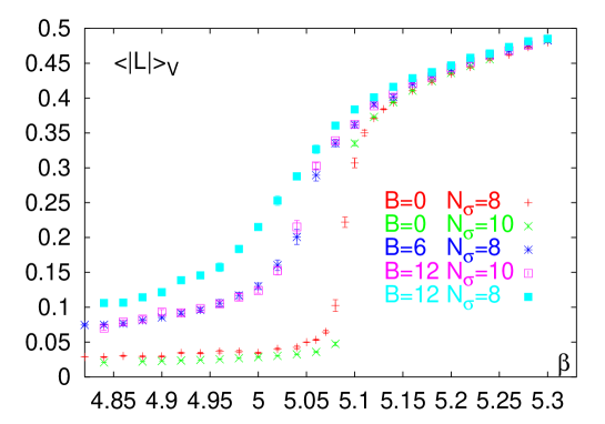
Figure 2: Polyakov loop expectation value for different values of $B$ and lattices with spatial extent $N_{\sigma}=8$ and 10.

For $B=0$ there is a clear signal for a first order phase transition which leads to a discontinuity in $\langle L\rangle$. For all $B>0$ we clearly observe a transition from a low temperature phase with small Polyakov loop expectation value to the high temperature regime characterized by a large Polyakov loop expectation value, which is similar to that of the $B=0$ case. The transition occurs in a temperature interval that broadens with increasing baryon number density. There is no indication for a discontinuous transition. In fact, this is not to be expected in a canonical calculation, even if the transition is first order. By changing the gauge coupling $\beta$ we vary the lattice cut-off and through this also the baryon number density continuously. At fixed non-zero baryon number we therefore follow a simulation path that traverses continuously through a region of two coexisting phases. This situation is schematically illustrated in Figure 3.

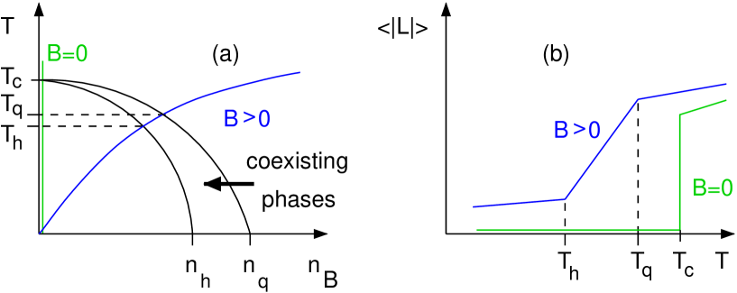
Figure 3: Schematic plot of the QCD phase diagram (a) in the temperature-baryon number density plane for the case of first order transitions in the entire plane. For $B>0$ and $T_{h}<T<T_{q}$ the system stays in a region of two coexisting phases. For $B=0$ the transition occurs at a unique temperature $T_{c}$. In (a) we also show the paths followed when varying the coupling $\beta$ in a Monte-Carlo simulation with fixed $B$, $N_{\sigma}$ and $N_{\tau}$. In (b) the expected behaviour of the Polyakov loop expectation value along these paths of non-zero $B$ as well as for $B=0$ is shown.

The question now is whether the transition region really is a region of coexisting phases. In this case the values of thermodynamic observables result as the superposition of contributions from two different phases appropriately weighted by the fraction each phase contributes in the coexistence regime. In the infinite volume limit this could result in a discontinuous change of the slope of thermodynamic observables when entering and leaving the coexistence region (for an illustration see e.g. Figure 3b).

To gain further insight into the structure of this regime we also analyzed various susceptibilities. In Figure 4 we show the conventional Polyakov loop susceptibility,

$$\chi_{L}=N_{\sigma}^{3}\biggl{(}\langle|L|^{2}\rangle-\langle|L|\rangle^{2}\biggr{)}~{}~{},$$ (3.10)

as well as the derivative of $\langle|L|\rangle$ with respect to $\beta$,

$$\chi_{\beta}={\partial\langle|L|\rangle\over\partial\beta}=\langle|L|\cdot S_{G}\rangle-\langle|L|\rangle\langle S_{G}\rangle~{}~{}.$$ (3.11)

Both response functions reflect the existence of a transition region that becomes broader with increasing $n_{B}$. Compared to the behaviour at $B=0$ they also change continuously in this region. Such a behaviour might as well just correspond to a smooth crossover to the high temperature regime; a conclusion also drawn from the heavy quark simulations with non-zero chemical potential [7]. To establish the existence of a region of coexisting phases with certainty will thus require a further, detailed analysis of finite size effects.

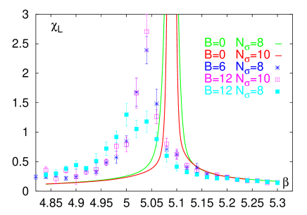
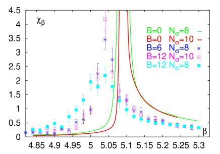
Figure 4: Polyakov loop susceptibility ($\chi_{L}$) and derivative of the Polyakov loop with respect to $\beta$ ($\chi_{\beta}$) for different values of $B$ and lattices with spatial extent $N_{\sigma}=8$ and 10. For $B=0$ we only show the Ferrenberg-Swendsen interpolations of the data for better visibility.

The width of the transition region gives some indication for the shift of the critical temperature when going from $B=0$ to a baryon number density which roughly corresponds to nuclear matter density. The gauge coupling at which the Polyakov loop expectation value starts rising rapidly is shifted from $\beta_{c}=5.09$ at $n_{B}/T^{3}\equiv 0$ to $\beta_{c}\simeq 4.95$ at $n_{B}/T^{3}=0.032$. A rough estimate based on the non-perturbative $\beta$-function for the $SU(3)$ gauge theory [19] suggests that this shift corresponds to a decrease of the critical temperature of about 15%.

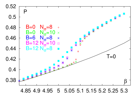
Figure 5: Plaquette expectation value for different values of $B$ and lattices with spatial extent $N_{\sigma}=8$ and 10. The solid line shows a spline interpolation for the zero temperature plaquette expectation value, $P_{0}$, calculated on an $8^{4}$ lattice.

The onset of deconfinement with increasing temperature is reflected in a sudden rise of bulk thermodynamic observables. For $B>0$ we thus expect to find a shift of this onset region to smaller temperatures. Otherwise, however, we expect that observables like e.g. the free energy density show a temperature dependence similar to that in the pure gauge sector. In the high temperature limit we expect to find a gluon gas slightly modified due to the presence of static quarks.

The free energy density can be calculated following the same approach used for $B=0$, i.e. through an integration over differences of plaquette expectation values calculated on asymmetric ($8^{3}\times 2$) and symmetric ($8^{4}$) lattices [19]. In Figure 5 we show the plaquette expectation value,

$$P={1\over 6N_{\sigma}^{3}N_{\tau}}\langle S_{G}\rangle~{}~{},$$ (3.12)

calculated for different values of $B$. The behaviour is similar to that of the Polyakov loop; with increasing $n_{B}$ the transition region broadens. The area between these data and the corresponding zero temperature results (solid line) increases. From this we obtain the free energy density,

$${f\over T^{4}}\Big{|}_{\beta_{0}}^{\beta}=~{}-6N_{\tau}^{4}\int_{\beta_{0}}^{\beta}{\rm d}\beta^{\prime}\bigl{[}P_{0}-P\bigr{]}~{}.$$ (3.13)

As can be seen from Figure 6 the free energy density decreases at fixed temperature with increasing $B$. This results in a shift of the onset of deconfinement to smaller temperatures. In the high temperature limit we indeed find that the free energy density is close to that of an ideal gluon gas at $B=0$. The contribution of static quarks remains small.

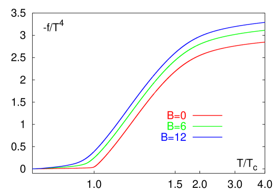
Figure 6: The negative of the free energy density in units of $T^{4}$ evaluated for different values of $B$ and lattices with spatial extent $N_{\sigma}=8$. The abscissa is a linear scale in terms of the gauge coupling $\beta$ covering the interval [4.74, 6.06]. We only show tick marks at the critical couplings on lattices with temporal extent $N_{\tau}=2,~{}3,~{}4,~{}6$ and 8, which correspond here to temperatures $T/T_{c}=1,~{}1.5,~{}2,~{}3$ and 4.

4 Conclusions

We have formulated the quenched limit of QCD at non-zero baryon number. Although this formulation still leads to a path integral representation of the partition function with an integrand that is not strictly positive it can be handled quite well numerically for moderate values of the baryon number. A first numerical simulation of the gluon thermodynamics in the background of static quarks shows the expected behaviour. We find indications for a region of coexisting phases, which broadens with increasing baryon number density. The critical temperature, at which the system enters this region, is shifted towards smaller temperatures with increasing baryon number density. At high temperature we recover the physics of a gluon gas similar to the $B=0$ case.

Although the transition clearly reflects the physics of deconfinement it may not be a true thermal phase transition that leads to discontinuous changes in thermodynamic observables. A clarification of this point will require calculations on larger lattices. If the statement turns out to be correct one may have to think about the deconfinement transition at non-zero baryon number in terms of a non-thermal percolation transition which anyhow seems to be a more appropriate physical picture for the deconfinement transition at zero temperature [9, 20].

We also find (indirect) evidence that the heavy quark potential does tend to a finite value at large distances already in the hadronic phase. The increase of the Polyakov loop expectation value with increasing baryon number density suggests that already at low temperatures string breaking starts at short distances. The heavy quark potential thus may be significantly modified in dense nuclear matter.

The formulation of quenched QCD in the presence of static quarks seems to be an appropriate model for the thermodynamics of QCD at non-zero baryon number. It may be similarly useful for the analysis of thermal properties of hadronic matter at non-zero density as the pure $SU(3)$ gauge theory has been for the understanding of the finite temperature deconfinement transition.

Acknowledgments:

This work was partly supported by the TMR network Finite Temperature Phase Transitions in Particle Physics, EU contract no. ERBFMRX-CT97-0122 and the DFG through grant no. KA 1198/4-1.

Appendix A Appendix

In this appendix we will derive the representation of $\hat{f}_{B}$ given in Eq. 2.19 and give the explicit representation of $\hat{f}_{B}$ for a few values of $B$.

The starting point for deriving Eq. 2.19 is the representation of $\hat{f}_{B}$ given in Eq. 2.18,

$$\hat{f}_{B} = (2\kappa)^{BN_{\tau}}\sum_{X}\prod_{k=1}^{B^{\prime}}\bar{D}_{n_{k}}(\vec{x}_{k})\quad,$$ (A.1)

where $B^{\prime}\leq B$ is the number of distinct sites $\vec{x}_{k}$ appearing in $X$ and $n_{k}$ is the quark occupation number for these distinct sites $\vec{x}_{k}$. They obey the constraint $\sum_{k}n_{k}=B$ with $0\leq n_{k}\leq 6n_{f}$.

Let us set up some general rules for the evaluation of $\hat{f}_{B}$. Any term in the sum appearing in Eq. A.1 is characterized by $6n_{f}$ numbers $k=(k_{1},...,k_{6n_{f}})$ where $k_{i}$ indicates how many sites are occupied $i$-times. The numbers $k_{i}$ are constrained by $\sum_{i}ik_{i}=B$. We thus may replace the vector $X=(\vec{x}_{1},...,\vec{x}_{B})$ by a vector $Y=(\vec{x}_{1},...,\vec{x}_{B^{\prime}})$ which only lists the distinct sites and is ordered according to the number of times these sites appear in $X$. The additional vector $k$ keeps track of this information, i.e. the first $k_{1}$ sites in $Y$ appear only once in $X$, from $k_{1}+1$ to $k_{1}+k_{2}$ we label the sites which appear twice in $X$ and so on. We then may write

$$\hat{f}_{B} = (2\kappa)^{BN_{\tau}}\sum_{Y,k}S_{k}(Y)\equiv(2\kappa)^{BN_{\tau}}\sum_{k}\bar{S}_{k}\quad.$$ (A.2)

with

$$S_{k}(Y)\equiv S_{(k_{1},...,k_{6n_{f}})}(Y)=\prod_{i=1}^{6n_{f}}\prod_{j=h_{i-1}+1}^{h_{i}}\bar{D}_{i}(\vec{x}_{j})~{}~{}.$$ (A.3)

Here $h_{0}=0$ and $h_{i}=\sum_{1\leq j\leq i}k_{j}$ and thus $h_{6n_{f}}=B^{\prime}$. Now we can perform the sum over $Y$ for a fixed set of occupation numbers for the $B^{\prime}$ distinct sites, which is given by the vector $k$,

$$\bar{S}_{k}\equiv\sum_{Y}~{}^{\prime}~{}S_{k}(Y)~{}~{}.$$ (A.4)

The prime on the sum reminds us that in doing this sum we have to avoid, of course, double counting. A pair of sites $\vec{x}_{i}\neq\vec{x}_{j}$ which have identical occupation numbers should appear only once in the sum, i.e. interchanging $\vec{x}_{i}$ and $\vec{x}_{j}$ should be counted as one configuration. This means that all $Y$ which only differ by a permutation within an interval $(h_{i}+1,h_{i+1})$ are equivalent. We can give up this restriction and divide by appropriate factors,

$$\bar{S}_{k}\equiv\biggl{(}\prod_{l=1}^{6n_{f}}k_{l}!\biggr{)}^{-1}\sum_{Y}S_{k}(Y)~{}~{}.$$ (A.5)

Now we only have to insure that all $\vec{x}_{i}\neq\vec{x}_{j}$. We also want to eliminate this restriction and do independent sums over all $\vec{x}_{i}$. This is achieved by performing one of the sums over $\vec{x}_{i}$ without any restriction and at the same time correct for the constraint by subtracting a term where two summation indices have been contracted. This process of factorization and contraction is repeated $(B^{\prime}-1)$ times. Let us illustrate this by doing the first step explicitly:

$$\sum_{Y}S_{k}(Y) = \sum_{\vec{x}_{1}\neq\vec{x}_{2}...\neq\vec{x}_{B^{\prime}}}\prod_{j=1}^{B^{\prime}}\bar{D}_{n_{j}}(\vec{x}_{j})$$

$$= \biggl{(}\sum_{\vec{x}_{1}}\bar{D}_{n_{1}}(\vec{x}_{1})\biggr{)}\biggl{(}\sum_{\vec{x}_{2}...\neq\vec{x}_{B^{\prime}}}\prod_{j=2}^{B^{\prime}}\bar{D}_{n_{j}}(\vec{x}_{j})\biggr{)}-$$

$$\sum_{t=2}^{B^{\prime}}\sum_{\vec{x}_{2}...\neq\vec{x}_{B^{\prime}}}\bar{D}_{n_{1}}(\vec{x}_{t})\prod_{j=2}^{B^{\prime}}\bar{D}_{n_{j}}(\vec{x}_{j})$$

$$= [\bar{D}_{n_{1}}]\sum_{\vec{x}_{2}...\neq\vec{x}_{B^{\prime}}}\prod_{j=2}^{B^{\prime}}\bar{D}_{n_{j}}(\vec{x}_{j})-\sum_{t=2}^{B^{\prime}}\sum_{\vec{x}_{2}...\neq\vec{x}_{B^{\prime}}}\bar{D}_{n_{1}}(\vec{x}_{t})\prod_{j=2}^{B^{\prime}}\bar{D}_{n_{j}}(\vec{x}_{j})\quad,$$

where $[...]$ denotes the sum over the lattice taken on a single configuration, i.e.

$$\biggl{[}\prod_{i}\bar{D}_{n_{i}}\biggr{]}=\sum_{\vec{x}}\prod_{i}\bar{D}_{n_{i}}(\vec{x})~{}~{}.$$ (A.6)

When continuing this process of factorization and contraction we arrive at a cluster decomposition of the $B^{\prime}$ factors we started with. Contracting two summation indices leads to a factor $(-1)$. We thus obtain a representation of $\hat{f}_{B}$ as a sum over products of clusters

$$F(\alpha)\equiv F(a_{1},...,~{}a_{6n_{f}})=(-1)^{(j-1)}\bigl{(}j-1\bigr{)}!\biggl{[}\prod_{l=1}^{6n_{f}}{\bar{D}_{l}^{a_{l}}\over a_{l}!}\biggr{]}\quad,$$ (A.7)

with

$$j=\sum_{l=1}^{6n_{f}}a_{l}\quad.$$ (A.8)

Here we have explicitly given the combinatorial factor for a cluster of length $j$, i.e.  a factor $(-1)$ for each of the $(j-1)$ contractions needed to generate a cluster of length $j$ and a factor $(j-1)!$ for the number of ways one can create such a cluster. We also included a combinatorial factor that takes into account that the permutation of $a_{l}$ factors $D_{l}$ appearing in a cluster does not lead to a new cluster decomposition.

In total there are $k_{l}!$ possibilities to distribute the various terms $D_{l}$. However, we have to take into account that each cluster can appear several times, i.e.  its degeneracy is $g_{(a_{1},...,~{}a_{6n_{f}})}$. Also the permutation of identical clusters does not lead to a new cluster decomposition. We thus arrive at the representation

$$\sum_{Y}S_{k}(Y)=\biggl{(}\prod_{l=1}^{6n_{f}}k_{l}!\biggr{)}\sum_{\{g_{\alpha}\}}\delta(\{g_{\alpha}\})\prod_{\{\alpha\}}\biggl{(}{1\over g_{\alpha}!}F(\alpha)^{g_{\alpha}}\biggr{)}\quad.$$ (A.9)

where $\alpha\equiv(a_{1},...~{}a_{6n_{f}})$ and the product runs over the set of vectors ${\alpha}$ which satisfy

$$\sum_{l=1}^{6n_{f}}la_{l}\leq B\quad.$$ (A.10)

Associated with each contributing vector $\alpha$ is a sum over the non-negative integers $g_{\alpha}$ which is symbolically represented in (A.9) by the sum over $\{g_{\alpha}\}$,

$$\sum_{\{g_{\alpha}\}}\equiv\sum_{g_{(1,0,...,0)}=0}^{B}\sum_{g_{(2,...,0)}=0}^{{\rm int}(B/2)}...\sum_{g_{\alpha}=0}^{i(\alpha)}...\quad,$$ (A.11)

where $i(\alpha)$ denotes the integer part of $B/\sum_{l=1}^{6n_{f}}la_{l}$. The Kronecker-$\delta$, $\delta(\{g_{\alpha}\})$, appearing in (A.9) summarizes the constraints the set of summation indices has to satisfy,

$$\delta(\{g_{\alpha}\})=\delta\biggl{(}B-\sum_{l=1}^{6n_{f}}lk_{l}\biggr{)}\prod_{l=1}^{6n_{f}}\delta\biggl{(}k_{l}-\sum_{\{\alpha\}}g_{\alpha}a_{l}\biggr{)}\quad.$$ (A.12)

We note that the combinatorial factor appearing in (A.9) in front of the sums will just cancel the factor appearing in (A.5); in fact, they do no longer depend on the actual choice of the vector $k$. We thus may easily sum over all possible vectors $k$ which yields essentially the result given in (A.9) with a less restrictive constraint on the possible choice of the summation indices $\{g_{\alpha}\}$,

$$\hat{f}_{B}=(2\kappa)^{BN_{\tau}}\sum_{\{g_{\alpha}\}}\delta\biggl{(}B-\sum_{l=1}^{6n_{f}}\sum_{\{\alpha\}}lg_{\alpha}a_{l}\biggr{)}\prod_{\{\alpha\}}\biggl{(}{1\over g_{\alpha}!}F(\alpha)^{g_{\alpha}}\biggr{)}\quad,$$ (A.13)

where the allowed set of numbers $\{\alpha\}$ is constrained only by (A.10).

This is the representation of $\hat{f}_{B}$ given in Eq. 2.19. In the following we will give the explicit representation for a few small values of $B$.

A.1 B=3

We get 3 contributions to $\hat{f}_{3}$:

$$\hat{f}_{3}=(2\kappa)^{3N_{\tau}}\biggl{(}\bar{S}_{001000}+\bar{S}_{110000}+\bar{S}_{300000}\biggr{)}\quad.$$ (A.14)

The terms $\bar{S}_{k}$ are sums over products of terms $D_{i}$ which are defined in Eq. 2.14. The three different contributions are given in Table 1.

$k$	$S_{k}(Y)$	$\prod k_{i}!$
001000	$\bar{D}_{3}(x_{1})$	1
110000	$\bar{D}_{1}(x_{1})\bar{D}_{2}(x_{2})$	1
300000	$\bar{D}_{1}(x_{1})\bar{D}_{1}(x_{2})\bar{D}_{1}(x_{3})$	3!

Table 1: 3-quark contributions

We thus obtain

$$\hat{f}_{3}=(2\kappa)^{3N_{\tau}}\biggl{(}[\bar{D}_{3}]-[\bar{D}_{1}\bar{D}_{2}]+{1\over 3}[\bar{D}_{1}^{3}]+[\bar{D}_{1}]([\bar{D}_{2}]-{1\over 2}[\bar{D}_{1}^{2}])+{1\over 6}[\bar{D}_{1}]^{3}\biggr{)}~{}~{}.$$ (A.15)

A.2 B=6

For $B=6$ one gets 11 contributions to $\hat{f}_{6}$:

$$\hat{f}_{6}=(2\kappa)^{6N_{\tau}}\sum_{k}\bar{S}_{k}\quad.$$ (A.16)

The different 6-vectors $k$ and the corresponding contributions $S_{k}(Y)$ are listed in the Table 2.

$k$	$S_{k}(Y)$	$\prod k_{i}!$
000001	$\bar{D}_{6}(x_{1})$	1
100010	$\bar{D}_{1}(x_{1})\bar{D}_{5}(x_{2})$	1
010100	$\bar{D}_{2}(x_{1})\bar{D}_{4}(x_{2})$	1
002000	$\bar{D}_{3}(x_{1})\bar{D}_{3}(x_{2})$	2!
200010	$\bar{D}_{1}(x_{1})\bar{D}_{1}(x_{2})\bar{D}_{4}(x_{3})$	2!
111000	$\bar{D}_{1}(x_{1})\bar{D}_{2}(x_{2})\bar{D}_{3}(x_{3})$	1
030000	$\bar{D}_{2}(x_{1})\bar{D}_{2}(x_{2})\bar{D}_{2}(x_{3})$	3!
301000	$\bar{D}_{1}(x_{1})\bar{D}_{1}(x_{2})\bar{D}_{1}(x_{3})\bar{D}_{3}(x_{4})$	3!
220000	$\bar{D}_{1}(x_{1})\bar{D}_{1}(x_{2})\bar{D}_{2}(x_{3})\bar{D}_{2}(x_{4})$	2! 2!
410000	$\bar{D}_{1}(x_{1})\bar{D}_{1}(x_{2})\bar{D}_{1}(x_{3})\bar{D}_{1}(x_{4})\bar{D}_{2}(x_{5})$	4!
600000	$\bar{D}_{1}(x_{1})\bar{D}_{1}(x_{2})\bar{D}_{1}(x_{3})\bar{D}_{1}(x_{4})\bar{D}_{1}(x_{5})\bar{D}_{1}(x_{6})$	6!

Table 2: 6-quark contributions

This again gives rise to contributions, which can be ordered according to the number of clusters contributing

$$\hat{f}_{6}=(2\kappa)^{6N_{\tau}}\sum_{i=1}^{6}a_{6}(i)~{}~{},$$ (A.17)

with

$$a_{6}(1) = -{1\over 6}[\bar{D}_{1}^{6}]+[\bar{D}_{1}^{4}\bar{D}_{2}]-{3\over 2}[\bar{D}_{1}^{2}\bar{D}_{2}^{2}]+{1\over 3}[\bar{D}_{2}^{3}]-[\bar{D}_{1}^{3}\bar{D}_{3}]+$$ (A.18)

$$2[\bar{D}_{1}\bar{D}_{2}\bar{D}_{3}]-{1\over 2}[\bar{D}_{3}^{2}]+[\bar{D}_{1}^{2}\bar{D}_{4}]-[\bar{D}_{2}\bar{D}_{4}]-[\bar{D}_{1}\bar{D}_{5}]+[\bar{D}_{6}]$$

$$a_{6}(2) = {1\over 18}[\bar{D}_{1}^{3}]([\bar{D}_{1}^{3}]-6[\bar{D}_{1}\bar{D}_{2}])+{1\over 2}[\bar{D}_{1}\bar{D}_{2}]^{2}+$$ (A.19)

$$[\bar{D}_{3}]({1\over 3}[\bar{D}_{1}^{3}]-[\bar{D}_{1}\bar{D}_{2}]+{1\over 2}[\bar{D}_{3}])-$$

$${1\over 2}(2[\bar{D}_{2}]-[\bar{D}_{1}^{2}])({1\over 2}[\bar{D}_{2}^{2}]+{1\over 4}[\bar{D}_{1}^{4}]-[\bar{D}_{1}^{2}\bar{D}_{2}]+[\bar{D}_{1}\bar{D}_{3}]-[\bar{D}_{4}])+$$

$$[\bar{D}_{1}]({1\over 5}[\bar{D}_{1}^{5}]-[\bar{D}_{1}^{3}\bar{D}_{2}]+[\bar{D}_{1}\bar{D}_{2}^{2}]+[\bar{D}_{1}^{2}\bar{D}_{3}]-[\bar{D}_{2}\bar{D}_{3}]-$$

$$[\bar{D}_{1}\bar{D}_{4}]+[\bar{D}_{5}])$$

$$a_{6}(3) = {1\over 48}(2[\bar{D}_{2}]-[\bar{D}_{1}^{2}])^{3}+$$ (A.20)

$${1\over 6}[\bar{D}_{1}](2[\bar{D}_{2}]-[\bar{D}_{1}^{2}])([\bar{D}_{1}^{3}]-3[\bar{D}_{1}\bar{D}_{2}]+3[\bar{D}_{3}])-$$

$${1\over 2}[\bar{D}_{1}]^{2}({1\over 2}[\bar{D}_{2}^{2}]+{1\over 4}[\bar{D}_{1}^{4}]-[\bar{D}_{1}^{2}\bar{D}_{2}]+[\bar{D}_{1}\bar{D}_{3}]-[\bar{D}_{4}])$$

$$a_{6}(4) = {1\over 16}[\bar{D}_{1}]^{2}(2[\bar{D}_{2}]-[\bar{D}_{1}^{2}])^{2}+{1\over 6}[\bar{D}_{1}]^{3}({1\over 3}[\bar{D}_{1}^{3}]-[\bar{D}_{1}\bar{D}_{2}]+[\bar{D}_{3}])$$ (A.21)

$$a_{6}(5) = {1\over 48}[\bar{D}_{1}]^{4}(2[\bar{D}_{2}]-[\bar{D}_{1}^{2}])$$ (A.22)

$$a_{6}(6) = {1\over 720}[\bar{D}_{1}]^{6}\quad.$$ (A.23)

These coefficients have been generated with Mathematica. In total there are 58 different terms contributing to $\hat{f}_{6}$. It is apparent that the number of terms increases rapidly with $B$. For $B=12$ and $n_{f}=1$ there are 58 different vectors $k$ which give rise to 2739 terms in $\hat{f}_{12}$.

References

- [1] J. Engels, R. Joswig, F. Karsch, E. Laermann, M. Lütgemeier and B. Petersson, Phys. Lett. B396 (1997) 210.
- [2] P. Hasenfratz and F. Karsch, Phys. Lett. 125B (1983) 308.
- [3] J. Kogut, M. Matsuoka, M. Stone, H.W. Wyld, J.H. Shenker, J. Shigemitsu and D.K. Sinclair, Nucl. Phys. B225 [FS9] (1983) 93.
- [4] I. Barbour, N.-E. Behilil, E. Dagotto, F. Karsch, A. Moreo, M. Stone and H.W. Wyld, Nucl. Phys. B275 [FS17] (1986) 296.
- [5] M.A. Stephanov, Phys. Rev. Lett. 76 (1996) 4472.
- [6] I. Bender, T. Hashimoto, F. Karsch, V. Linke, A. Nakamura, M. Plewnia, I.O. Stamatescu and W. Wetzel, Nucl. Phys. B (Proc. Suppl.) 26 (1992) 323.
- [7] T.C. Blum, J.E. Hetrick and D. Toussaint, Phys. Rev. Lett. 76 (1996) 1019.
- [8] J. Kertész, Physica A161 (1989) 58.
- [9] H. Satz, Nucl. Phys. A642 (1998) 130c.
- [10] D.E. Miller and K. Redlich, Phys. Rev. D35 (1987) 2524.
- [11] A. Roberge and N. Weiss, Nucl. Phys. B275 [FS17] (1986) 734.
- [12] I.M. Barbour, S.E. Morrison, E.G. Klepfish, J.B. Kogut and M.-P. Lombardo, Nucl. Phys. B (Proc. Suppl.) 60 (1998) 220.
- [13] F. Karsch and K.-H. Mütter, Nucl. Phys. B313 (1989) 541.
-
[14]
M. Alford, A. Kapustin and F. Wilczek ,
Phys. Rev. D59 (1999) 054502;
M. Alford, New Possibilities for QCD at finite Density, IASSNS-HEP-98-81, hep-lat/9809166. -
[15]
T. Matthews and A. Salam, Nuovo Cim. 12 (1954) 563; 2 (1955) 120;
C. Lang and H. Nicolai, Nucl. Phys. B200 (1982) 135. - [16] B. Berg, J. Engels, E. Kehl, B. Waltl and H. Satz, Z. Phys. C31 (1986) 167.
- [17] K.G. Wilson, Phys. Rev. D10 (1974) 2445.
- [18] C. DeTar, O. Kaczmarek, F. Karsch and E. Laermann, Phys. Rev. D59 (1999) 031501.
- [19] G. Boyd, J. Engels, F. Karsch, E. Laermann, C. Legeland, M. Lütgemeier and B. Petersson, Nucl. Phys. B469 (1996) 419.
- [20] T. Celik, F. Karsch and H. Satz, Phys. Lett. 97B (1980) 128.