FTUAM-99-6; IFT-UAM/CSIC-99-8 INLO-PUB-6/99

Abstract: We discuss the manifestation of instanton and monopole solutions on a periodic lattice at finite temperature and their relation to the infinite volume analytic caloron solutions with asymptotic non-trivial Polyakov loops. As a tool we use improved cooling and twisted boundary conditions. Typically we find $2Q$ lumps for topological charge $Q$. These lumps are BPS monopoles.

1 Introduction

Calorons are characterised by their holonomy, defined by the value of the Polyakov loop at spatial infinity. When non-trivial, it resolves the fact that a caloron is built from constituent monopoles, their mass ratios directly determined by the holonomy [1, 2]. These solutions differ from the (deformed) instantons described by the Harrington-Shepard solution [3], for which the holonomy is trivial. What we find by (improved [4]) cooling on a finite lattice, to relatively high accuracy, is $SU(2)$ configurations that fit these infinite volume caloron solutions for arbitrary constituent monopole mass ratios. Twist [5] in the time direction constrains the masses of the two constituent monopoles to be equal.

The constituent nature becomes evident when the instanton scale parameter $\rho$ is larger than the time extent $\beta$ (inverse temperature) of the system. The masses of the monopoles are for $SU(2)$ proportional [1] to $\omega$ and ${\scriptstyle{{1\over 2}}}-\omega$, where $\omega$ ($0\leq\omega\leq{\scriptstyle{{1\over 2}}}$) follows from the trace of the holonomy: $2\cos(2\pi\omega)$. The distance between the monopole constituents is given by $\pi\rho^{2}/\beta$. At $\rho/\beta\ll 1$ the constituents therefore hide deep inside the core of the instanton and the non-trivial holonomy plays no discernible role. But for $\rho/\beta\gg 1$ the situation is opposite; the instanton becomes static and will dissolve in two BPS monopoles [6, 7]. The transition occurs [8, 9] for ${\scriptstyle{{1\over 2}}}\beta<\rho<\beta$. When, however, the holonomy is trivial one of the monopoles is massless and will hide in the background.

Charge one $SU(N)$ calorons have $N$ constituent monopoles [10] for non-trivial holonomy. These have the same location in time, but the spatial position of each constituent monopole can be arbitrary. There are (at fixed holonomy) $N-1$ phases associated to the residual $U(1)^{N-1}$ gauge symmetry that leaves the holonomy invariant. The total number of parameters describing these calorons is therefore $4N$. One may speculate that the $N-1$ phases are replaced in a finite volume by the holonomy itself, indeed described by $N-1$ eigenvalues taking values in $U(1)$ ($\exp(2\pi i\omega)$ for $SU(2)$). Also it is likely that, in general, a charge $Q$ caloron is characterised by $NQ$ constituent monopoles, which we confirm for a $Q=2$ caloron solution obtained from cooling. At zero temperature it is tempting to explain the $4NQ$ parameters of an $SU(N)$ charge $Q$ instanton in terms of the positions of $NQ$ objects [11]. Indeed, there are charge $Q=1/N$ instanton solutions on a torus with twisted boundary conditions, whose four parameters specify its position [12]. Subdividing a given finite volume in boxes with the appropriate twisted boundary conditions, such that each cell supports a $Q=1/N$ instanton, provides an exact solution that has $NQ$ lumps. In ref. [11] it is suggested that a typical self-dual configuration would appear as an ensemble of $N$ randomly placed lumps of charge $Q=1/N$, whose locations would account for the $4NQ$ parameters. The results at finite temperature presented here suggest that the assignment of $Q=1/N$ charge to each lump might only hold on the average.

Our results point to the usefulness of studying the dynamical role of these configurations. A first attempt in that direction is hampered by the fact that at high temperatures where the constituent monopoles should be well separated, the fluctuations are so large that on average topological charge cannot be supported over large enough domains of space-time to capture the configurations with cooling [13].

On a semiclassical basis one is tempted to argue against non-trivial holonomy. It polarises the vacuum at infinity and raises the energy density above the one with a trivial holonomy [14]. But now we have seen that these BPS bound states can be supported in a finite volume, it is time to acknowledge this as an irrelevant objection, given the non-perturbative and non-trivial nature of the QCD vacuum. As a consequence, constituent monopoles, at least at high temperatures, are tangible objects that do not depend on a choice of Abelian projection [15], which till now has been used to address the monopole content of the theory [16]. In extracting the non-trivial topological content of the theory constituent monopoles introduce an extra parameter: their mass, $16\pi^{2}\omega/\beta$. Up to now only the maximal mass, $8\pi^{2}/\beta$, of such a BPS monopole was considered. It arises in terms of the caloron with trivial holonomy, described by the Harrington-Shepard solution [3]. Rossi [17] showed that at high temperature, equivalent to a large scale parameter, this solution indeed becomes a BPS monopole [7].

In section 2 we discuss the numerical procedure of constructing the configurations. Apart from cooling with improved actions, twisted boundary conditions are used as a tool for biasing the cooling towards non-trivial holonomy. The twist can then be removed, while preserving the non-trivial holonomy and the constituent monopole nature of the configuration, although it should be pointed out that no exact charge one instanton solutions can exist on $T^{4}$, which remains true at finite temperature. Interesting in this respect is that the well-established $Q=1/2$ instanton solutions that occur with suitable combinations of spatial and temporal twists (so-called non-orthogonal twist), can be argued to become a single static BPS monopole in the infinite volume limit at finite temperature. This is discussed in section 3. Configurations of higher charge are discussed in section 4 and we conclude with some speculations and possible applications. An appendix summarises the formulae for the $SU(2)$ analytic caloron solutions.

2 Non-trivial holonomy from time-twist

For finite temperature ($T=1/\beta$) and volume ($L^{3}$, $L\gg\beta$) caloron configurations with non-trivial holonomy were discovered on lattices with twisted boundary conditions. Starting with a random configuration and after applying a standard cooling algorithm one frequently reaches $Q=1$ self-dual configurations which are stable under many cooling steps. These configurations are later analysed. An automatic peak-searching routine identified one or (actually more frequently) two lumps in them. These are our candidate caloron configurations on the lattice. Below, we will show how twist in the time direction can help in bringing about non-trivial holonomy.

To appreciate the ease with which twist can be implemented on the lattice, and because twist has been a very useful tool [4, 18, 19], neglected by large parts of the lattice community, we think it is useful to review the notion of twist-carrying plaquettes that introduce twist by modifying the lattice action [20], but not the measure. In the initial formulation of ’t Hooft [5], $SU(N)$ twisted boundary conditions were implemented by defining gauge functions $\Omega_{\mu}(x)$ (which are assumed independent of $x_{\mu}$), such that with $a^{\mu}$ the periods of the torus in the four directions ($a_{\mu}^{\nu}=L_{\mu}\delta_{\mu\nu}$)

$$U_{\nu}(x+a^{\mu})=\Omega_{\mu}(x)\,U_{\nu}(x)\,\Omega^{\dagger}_{\mu}(x+\hat{\nu}),$$ (1)

here re-formulated for a lattice of size $\prod_{\mu}N_{\mu}$. Calculating $U_{\nu}(x+a^{\mu}+a^{\lambda})$ in two ways shows that for all $x$ one should have

$$\Omega_{\mu}(x+a^{\lambda})\,\Omega_{\lambda}(x)=Z_{\mu\lambda}\,\Omega_{\lambda}(x+a^{\mu})\,\Omega_{\mu}(x),$$ (2)

with $Z_{\mu\lambda}=\exp(2\pi in_{\mu\lambda}/N)$ an element of the center of the gauge group. (We define $k_{i}=n_{0i}$ and $m_{i}={\scriptstyle{{1\over 2}}}\varepsilon_{ijk}n_{jk}$ to distinguish the twist in the time and space directions respectively). The center freedom arises because $U_{\mu}(x)$ is invariant under constant center gauge transformations (i.e. the gauge field is in the adjoint representation). In the presence of site variables (fields in the fundamental representation) one is required to put all $Z_{\mu\nu}$ equal to 1. We now perform the following change of variables [20]

$$U^{\prime}_{\mu}(x)=U_{\mu}(x)\,\Omega_{\mu}(x),\quad\mbox{for}\quad x_{\mu}=N_{\mu}-1.$$ (3)

As a consequence, the plaquettes at $x_{\lambda}\!=\!N_{\lambda}-1$ and $x_{\mu}\!=\!N_{\mu}-1$ (for any value of the other two components of $x$) can be shown to have acquired an additional factor $Z_{\lambda\mu}$. These corner plaquettes are called twist-carrying and the change of variables has absorbed the twist in the action, by multiplying these plaquettes by the appropriate center element (the action involves the real part of the plaquette variables after this multiplication). The location of the twist-carrying plaquette is arbitrary, as one is free to choose the boundary of the box used for defining the torus. Alternatively, the twist-carrying plaquette can be moved around by a periodic gauge transformation. It corresponds to the non-Abelian analogue of a Dirac string, and is at the heart of ’t Hooft’s definition of magnetic flux for non-Abelian gauge theories [21, 5]. Thus, twist is introduced by the trivial modification of the weights of the plaquettes in terms of multiplication with appropriate center elements and causes no computational overhead.

Note that we have just shown that if $Z_{\mu\nu}=1$ for all $\mu$ and $\nu$, in a suitable gauge the links can be chosen periodic without changing the weights of the plaquettes. In the continuum, however, there remains an obstruction in making the gauge field periodic when the topological charge of the configuration is non-trivial [22, 18]. This shows that on the lattice, only the center charges are unambiguously defined. Interestingly this includes configurations [12] that in the continuum would be assigned a non-trivial fractional Pontryagin index [5] (so-called twisted instantons).

To understand what the effect of the twist is on the holonomy, we use the observation that the presence of the $Z_{N}$ flux can be measured by taking a Polyakov loop in the $a^{\lambda}$ direction, which when translated over a period in the $a^{\mu}$ direction picks up a factor $Z_{\mu\lambda}$.

$$P_{\lambda}(x)=\frac{1}{N}{{\rm Tr}~{}P}\exp\left(\int_{0}^{1}A_{\lambda}(x+sa^{\lambda})ds\right)\Omega_{\lambda}(x),\quad P_{\lambda}(x+a^{\mu})=Z_{\lambda\mu}P_{\lambda}(x).$$ (4)

There are various ways to see this [23, 4], but becomes most evident when ‘pulling’ the loop over the twist-carrying plaquette. For $SU(2)$ this means that the Polyakov loop is anti-periodic in case the twist is non-trivial. In particular for $Z_{0i}=-1$, $P_{0}(\vec{x})$ is anti-periodic in the $x_{i}$-direction. As we increase the size of the spatial torus it is natural to expect that the self-dual configuration would approach a caloron solution. Then $P_{0}(\vec{x})$ would approach a constant at spatial infinity. This is only compatible with the anti-periodicity implied by the non-trivial time-twist when $P_{0}(\vec{x})\rightarrow 0$ for $|\vec{x}|\rightarrow\infty$, forcing $\omega={\scriptstyle{{1\over 4}}}$ and thus non-trivial holonomy. This therefore provides a sure way of obtaining caloron solutions with non-trivial holonomy on the lattice, which at high temperature gives rise to two constituent monopoles, albeit in this case of equal mass.

Since the twist in the time direction forces the constituent monopoles to have equal mass, the lattice corrections to the value of the action (which depend on the shape of the configuration [4]) are affected only by the separation of the two constituents (in the next section we will encounter the situation where the mass ratio is affected by the cooling). This allows to manipulate the positions of the two lumps by using the tool of cooling with modified actions. This can be implemented [4] by using a lattice action that combines the traces of the $1\!\times\!1$ and $2\!\times\!2$ plaquettes. The two couplings are fixed in terms of the parameters multiplying the leading (continuum) and next to leading ($a^{2}$) terms in the expansion of the lattice action in powers of the lattice spacing $a$. The $a^{2}$ term is given by a unique dimension six operator, and its coefficient is called $\varepsilon$ (it is trivial to incorporate the twist-carrying plaquettes also in these modified actions). Wilson’s action corresponds to $\varepsilon\!=\!1$. The choice $\varepsilon<1$ is known as over-improvement, whereas improved cooling is performed by choosing $\varepsilon\!=\!0$. In this last case the lattice and continuum action differ only by corrections of order $a^{4}$. For that reason, we will choose $\varepsilon\!=\!0$ whenever we compare with the analytic infinite volume continuum caloron solution. However, unlike for the continuum action, the value of the $a^{2}$ operator depends on the position of the constituent monopoles, and therefore we can use other values of $\varepsilon$ to alter these positions. Cooling with the Wilson action has the effect of driving the constituent monopoles together, since the Wilson action is decreased with respect to the continuum when the field strength has a larger gradient [4]. Once the two lumps merge, and can no longer be distinguished from an instanton (at which point the solution will no longer be static), it follows the usual fate of an instanton under prolonged cooling with the Wilson action: At some point it falls through the lattice [24]. (For cooling histories see fig. 3).

Over-improved cooling has the effect of pushing the two constituent monopoles apart. One can speed-up the rate at which monopoles separate by decreasing $\varepsilon$. Apriori it is not clear if, when the lumps are maximally apart, the solution will not be affected significantly by the boundary conditions. This will partly depend on the ratio $L/\beta$, but we find for $L=4\beta$ that these effects are rather small.

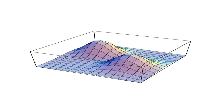
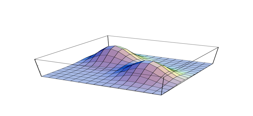
Figure 1: Lattice caloron profiles (left) on a $16^{3}\times 4$ lattice for $\vec{k}=(1,1,1)$, created with improved cooling ($\varepsilon=0$). The total action is $1.000185\times 8\pi^{2}$. Vertically is plotted $\log(1+s/3)$, with $s$ the action density at the lattice site (after clover averaging). The profile fits well to the analytic caloron solution (shown on the right at $y\!=\!t\!=\!0$) with $\omega={\scriptstyle{{1\over 4}}}$ and constituents at $\vec{y}_{1}=(2.50,0.12,0.95)$ and $\vec{y}_{2}=(1.38,-0.24,2.67)$, in units where $\beta=1$ (or $a={\scriptstyle{{1\over 4}}}$) and the left most lattice point corresponding to $x=z=0$.

In figure 1 we give an example of a caloron configuration with well separated constituents on a $16^{3}\!\times\!4$ lattice with $\vec{k}=(1,1,1)$, initially generated by cooling with the Wilson action, switching to improved cooling to reduce lattice artifacts. Shown is the action density $s$. We see that the agreement with the infinite volume analytic result is very good, with the action peaks for the lattice result somewhat lower (this feature is somewhat suppressed by plotting $\log(1+s/3)$, rather than $s$). The total action of this static lattice configuration is very close to the required continuum value $8\pi^{2}$. An example of a non-static configuration with overlapping constituents will be presented below (see fig. 5). There seems no doubt that a continuum solution with this constituent monopole structure should exist on the time-twisted torus.

3 The case of space-twist

When both space and time twists are non-trivial and $\vec{k}\cdot\vec{m}\!\neq\!0~{}{\rm mod}~{}N$ (called non-orthogonal twist), the minimum of the action corresponds to a so-called twisted instanton with fractional charge. Unlike the integer charge instantons, these twisted instantons can not fall through the lattice. Their scale is fixed, only their position is a free parameter. This was used in the past [12] to find accurate lattice results using ordinary cooling ($\varepsilon\!=\!1$). At high temperatures such a twisted instanton becomes static and represents a single BPS monopole on $T^{3}$. The twist allows for non-zero charge in the box. As discussed in the previous section it also gives rise to a holonomy characterised by $\omega={\scriptstyle{{1\over 4}}}$. Indeed, we were able to fit the finite temperature twisted instanton (in a sufficiently large volume) to one of the constituent monopoles of the caloron at $\omega={\scriptstyle{{1\over 4}}}$ (when placing the other constituent at a sufficiently large separation). In the appropriate limits both become ordinary BPS monopoles with mass $4\pi^{2}/\beta$.

Figure 2: Lattice minimum action for various sizes (left), including the best fit to eq. (5) with: $S_{0}=0.999975(4)$, $b=0.19950(7)$, $c=0.3107(3)$ and $d=0.0844(5)$. Also shown is the lattice action profile ${\cal E}(x)$, obtained by summing the action density over all but one of the spatial coordinates, as compared to the infinite volume analytic BPS result (right).

Now we will show the type and size of finite volume and lattice artifact effects. In fig. 2 (left) we display a plot of the minimum lattice (Wilson) action for lattices with different space and time extensions, $N_{s}^{3}\!\times\!N_{t}$ and twist $\vec{k}\!=\!\vec{m}\!=\!(1,1,1)$. In the given range, $N_{t}=4$—$7$ and $N_{s}=16$—$32$, deviations from the continuum result are of the order of a few percent. However, the pattern of deviations from the continuum value is well understood. If we set $a_{t}=1/N_{t}$ and $a_{s}=1/N_{s}$, the value of the lattice action can be fitted with great accuracy to a formula:

$$S/4\pi^{2}=S_{0}-ba_{t}^{2}-ba_{s}^{2}-ca_{t}a_{s}-d(a_{t}+a_{s})^{4}.$$ (5)

The extrapolated value of the continuum action matches $4\pi^{2}$ to a precision of a few parts in $10^{5}$. Notice also that the extrapolation shows the existence of a self-dual continuum solution for any value of the ratio $L/\beta\!=\!N_{s}/N_{t}$. Furthermore, the lattice correction to the action decreases in absolute value with the ratio $N_{s}/N_{t}$, consistent with the statement made before that Wilson’s action decreases with decreasing separation of the monopoles, since in this case $N_{s}$ plays the role of the separation between lumps (the periodic mirrors).

To measure finite volume corrections, we performed improved cooling ($\varepsilon\!=\!0$, to minimise lattice corrections) for $N_{s}\!=\!16$ and $32$. In this case, the values of the minimum lattice action attained are of the order $S/4\pi^{2}\!=\!1.0001(1)$. In fig. 2 (right) we compare the $x$-profiles ${\cal E}(x)$ obtained from the lattice minimum action configuration with the corresponding one for the BPS monopole. The $x$-profile is the integral of the action density over all but the $x$ coordinate. This quantity has smaller errors and is less sensitive to the lattice discretisation than the action density itself. From the figure we see how the lattice profiles approach the infinite volume BPS monopole profile. The slow convergence is due to the powerlike Abelian tail of the BPS monopole (in contrast to the exponential tail found for other cases [25]).

Interestingly, an exact caloron solution with equal-size constituents ($\omega={\scriptstyle{{1\over 4}}}$) on the twisted torus can be constructed by gluing two twisted instantons together, starting from the $Q={\scriptstyle{{1\over 2}}}$ solution defined by $\vec{k}=\vec{m}=(1,0,0)$. Gluing two boxes in the $y$- or $z$-directions preserves $\vec{k}$, but reduces $\vec{m}$ to the trivial value (since $n_{\mu\nu}$ is defined modulo 2 for $SU(2)$). This exact solution corresponds to the situation studied in the previous section. Instead, gluing two boxes in the $x$-direction removes the time-twist, but preserves the space-twist. The same twist results when gluing the two boxes in the time-direction. In the first case we have an exact solution on a space-twisted torus with equal size constituents (corresponding to $\omega={\scriptstyle{{1\over 4}}}$) at maximal separation in the direction of the twist, whereas in the second case the static nature of the finite temperature solution simply leads to doubling the mass of the monopole. Therefore this solution corresponds to an exact caloron solution on a space-twisted torus with trivial holonomy (the other constituent monopole is massless).

Figure 3: Cooling histories for $(\vec{m},\vec{k})=(\vec{0},\vec{1})$ and $(\vec{1},\vec{0})$ (resp. thin and fat curves), where $\vec{1}\equiv(1,1,1)$, on lattices of size $16^{3}\times 4$. Solid, dashed and dotted curves are for resp. $\varepsilon=0,1,-1$ cooling. For $(\vec{0},\vec{1})$, where $\omega\equiv{\scriptstyle{{1\over 4}}}$, the two $\omega$–curves cannot be distinguished.

We have also performed lattice studies on a space-twisted torus, with $\vec{k}=\vec{0}$, which allowed us to probe the constituent monopole mass ratios, by a subtle use of the cooling procedure. It can be proven that without twist there are no regular charge one instanton solutions on a torus [26], but for any non-trivial twist an 8 dimensional space of regular solutions exists [27, 28]. Part of this parameter space comes about by gluing a localised instanton to the unique curvature free background supported by the twist. The eight parameters are given by scale, space-time position and so-called attachment parameters, that describe the gauge orientation of the localised instanton relative to the fixed curvature free background. For $\vec{m}\neq\vec{0}$ we find that the magnetically charged constituent monopoles, superposed on this non-Abelian magnetic flux background, experience an additional force that repels them as far as the finite volume allows. The presence of this force is evident from the fact that under prolonged cooling in all cases, $\varepsilon=1,0,-1$, the separation between the two constituent monopoles was increasing and that their centers lined up with the direction of $\vec{m}$. Once the constituent monopoles are placed at their maximal separation, further cooling with the Wilson action ($\varepsilon\!=\!1$) leads to action shifting from one to the other peak, driving the constituent monopole mass ratios away from equal masses. Once one of the masses has decreased to zero, the scale parameter of the remaining (deformed) instanton configuration can shrink, resulting in the usual fate of falling through the lattice under prolonged cooling with the Wilson action. For over-improvement the effect is opposite, and the masses are pushed to equal values. The ‘force’ —due to lattice artifacts— changing the value of $\omega$ can be neglected for $\varepsilon\!=0$ cooling. We summarise the behaviour under cooling in fig. 3, by showing the distance between the peak locations and $\omega$ (estimated by equating $({\scriptstyle{{1\over 2}}}\!-\!\omega)^{4}/\omega^{4}$ to the ratio of the peak heights) as a function of the number of cooling sweeps. Shown are the histories for $\vec{m}\!=\!(1,1,1)$ at $\varepsilon\!=\!-1,0,1$ and for $\vec{k}\!=\!(1,1,1)$ at $\varepsilon\!=\!0,1$.

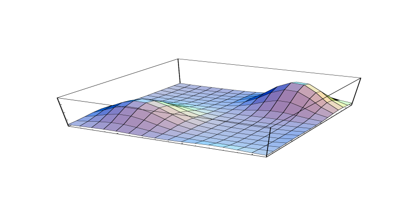
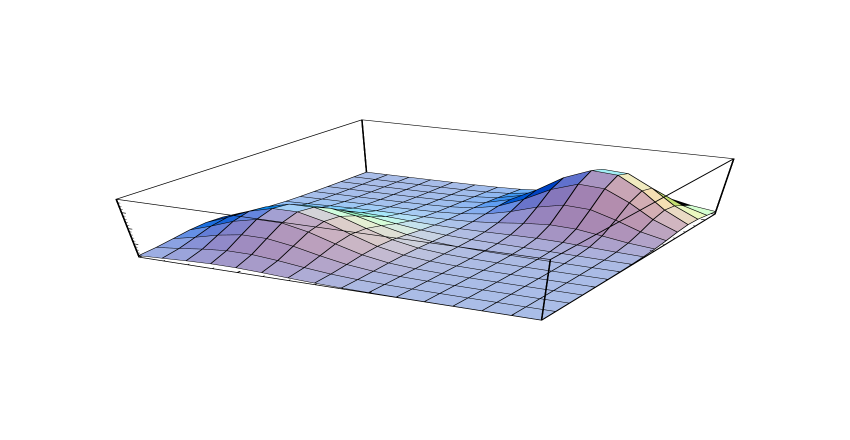
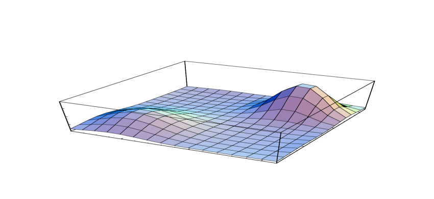
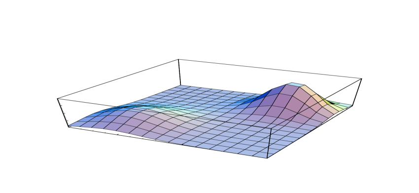
Figure 4: Lattice caloron profiles (left) for two configurations on a $16^{3}\times 4$ lattice for $\vec{m}=(1,1,0)$, created with improved cooling ($\varepsilon=0$) - after manipulating with $\varepsilon=\pm 1$ cooling to obtain the desired mass ratios. The total actions are $1.000155\times 8\pi^{2}$ (top) and $1.000001\times 8\pi^{2}$ (bottom). Vertically is plotted $\log(1+s/3)$, with $s$ the action density at the lattice site (after clover averaging). The profiles fit well to the analytic caloron solutions (shown on the right at $y=t=0$) with top: $\omega=0.210$ and constituents at $\vec{y}_{1}=(1.04,-0.08,0.86)$ and $\vec{y}_{2}=(3.05,-0.09,2.85)$, and bottom: $\omega=0.175$ with constituents at $\vec{y}_{1}=(0.85,-0.06,0.85)$ and $\vec{y}_{2}=(2.85,-0.06,2.85)$, all in units where $\beta=1$ (or $a={\scriptstyle{{1\over 4}}}$) and the left most lattice point corresponding to $x=z=0$.

That we can have solutions that are characterised by arbitrary mass ratios of the constituent monopoles is also illustrated in figure 4, which represents two values for the parameter $\omega$, comparing the finite volume configurations obtained from improved cooling to the analytic infinite volume caloron solutions with non-trivial holonomy. We see again that the agreement is very good (and will improve for increasing $L/\beta$), with the peaks for the lattice result now somewhat higher as compared to the infinite volume results.

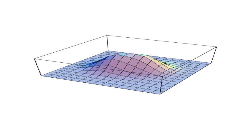
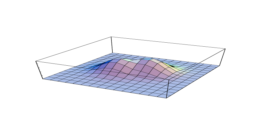
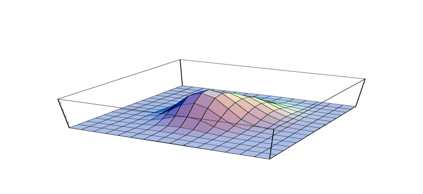
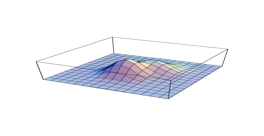
Figure 5: Caloron profile for two configurations (left and right) on a $16^{3}\times 4$ lattice for $\vec{m}=\vec{0}$ obtained with improved ($\varepsilon=0$) cooling. Vertically is plotted $\log(1+s/3)$, with $s$ the action density at the lattice site (after clover averaging). The top plot corresponds to the plane $y=t=0$ and the bottom one to $y=0$, $t={\scriptstyle{{1\over 2}}}$. Left: $\vec{k}=(1,1,1)$ with total action $1.000016\times 8\pi^{2}$, $\omega={\scriptstyle{{1\over 4}}}$, $t_{0}=-0.125$, $\vec{y}_{1}=(1.75,-0.15,1.43)$ and $\vec{y}_{2}=(2.20,0.00,2.20)$. Right: $\vec{k}=(0,0,0)$ with total action $1.010951\times 8\pi^{2}$, $\omega=0.185$, $t_{0}=-0.09$, $\vec{y}_{1}=(2.29,0.07,2.15)$ and $\vec{y}_{2}=(1.57,0.08,1.73)$. All coordinates obtained from fitting to the infinite volume analytic solutions (not shown) are in units where $\beta=1$ (or $a={\scriptstyle{{1\over 4}}}$) and the left most lattice point corresponding to $x=z=0$.

Next, we discuss the comparison with configurations that are not static. Here the constituents are close together and therefore there is considerable overlap. This is illustrated in figure 5, both in the case of twist in time as in the case of no twist. As mentioned previously, the presence of twist in time ($\vec{k}\neq 0$) forces $\omega={\scriptstyle{{1\over 4}}}$, while in the absence of twist $\omega$ can be arbitrary. Obtaining configurations with no twist requires some care. By cooling random configurations one ends up quickly in the trivial vacuum configuration. Hence, it is useful to start with a $Q=1$ configuration having $\vec{m}\neq\vec{0}$ obtained by cooling. Then twist is eliminated from this configuration by setting the weights of the twist-carrying plaquettes to their standard (untwisted) value. Additional improved cooling steps were applied to the configuration, leading to a new solution still having a non-trivial $\omega$ value. We recall that there are no exactly self-dual $Q=1$ solutions on the torus without twist [26]. However, for solutions well-localised inside the torus the configuration is very approximately self-dual. Notice, nonetheless, that this reflects itself in higher values of the minimum lattice action. For these configurations with periodic boundary conditions performing further cooling steps with positive or zero $\varepsilon$ will bring the constituents together and leads to the standard fate of instantons on the lattice. This can be stabilised by $\varepsilon<0$, and the better the solution is contained within the box, the closer one can take $\varepsilon=0$ to have a stable lattice solution [4].

The differences with the analytic infinite volume caloron solutions only show themselves by small differences in peak heights (at $t=0$) and would not be clearly visible on the scale of figure 5. Instead, in figure 6, we display the analytic action density profile in the $z-t$ plane, where $z$ is the axis connecting the two constituent monopole centers. The values of $\omega$ and the distance of the constituent monopoles is as in figure 5. It is clear that a two-lump structure is still visible. As a function of $z$ the constituent monopoles are best seen for $t$ values where the density is minimal ($t={\scriptstyle{{1\over 2}}}$). The logarithmic scale enhances the regions of low action densities in favour of those with large densities, and brings out more clearly the constituents.

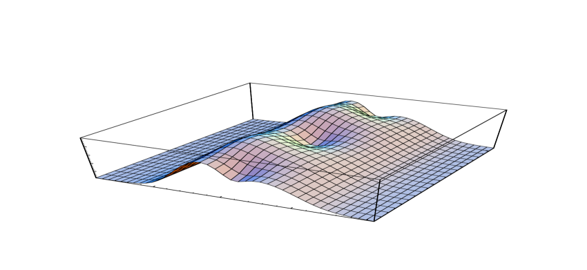
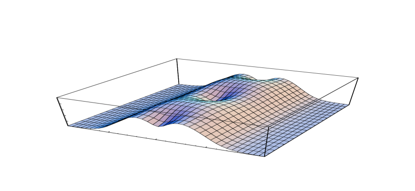
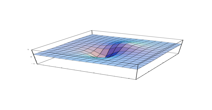
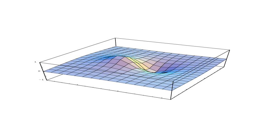
Figure 6: Space-time profile for the calorons of figure 5, using the infinite volume analytic result. Vertically is plotted $\log(1+s/3)$, with $s$ the action density. Horizontally is plotted time ranging over two periods $\beta=1$ and space along the line connecting the two constituent monopole positions. Left corresponds to $\omega={\scriptstyle{{1\over 4}}}$ and right to $\omega=0.185$.

Figure 7: Profile of the Polyakov loop $P_{0}(\vec{x})$ for the calorons of fig. 5. Left corresponds to $\vec{k}=(1,1,1)$ and $\omega={\scriptstyle{{1\over 4}}}$, right is for $\vec{k}=(0,0,0)$ with $\omega=0.185$. Plotted is the plane $y=0$, for other details see the caption of fig. 5.

For large $L/\beta$ the difference between the finite volume solutions with respect to the infinite volume calorons is mostly due to the contribution of the Coulombic tails of the periodic copies of the monopole constituents. That this depends on the nature of the twist is to be expected. For twist in time the charges change sign when shifting over a period of the torus. For twist in space there is no change in sign. This behaviour of the charges is correlated to the zeros of $A_{0}$ (which plays the role of the Higgs field) at the core of the constituent monopoles as illustrated by the behaviour of $P_{0}$ which is anti-periodic with time-twist and periodic with space-twist. It can be shown from the analytic solution (see the Appendix) that $P_{0}=1$ (corresponding to $A_{0}=0$) near one of the constituent centers, and $P_{0}=-1$ near the other (related to $A_{0}=0$ by a gauge transformation that is anti-periodic in time - the gauge transformation that changes $\omega$ to ${\scriptstyle{{1\over 2}}}-\omega$). This vanishing, i.e. $P_{0}^{2}=1$, of the Higgs field near to the constituent monopole centers is reproduced by the lattice data as is illustrated in figure 7.

4 Higher charge calorons

In this section we discuss our finding for higher topological charge. Analytic results in infinite volumes for higher charge calorons with non-trivial holonomy are not yet available.

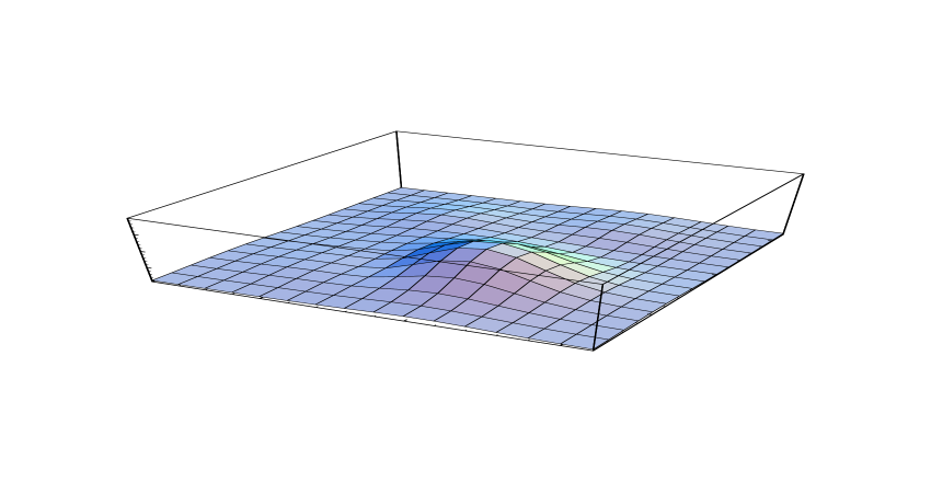
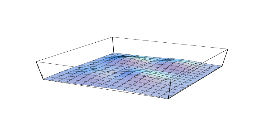
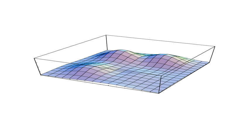
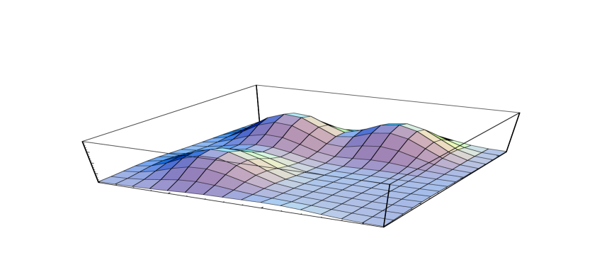
Figure 8: Lattice action density profiles of a (static) charge 2 configuration found with ordinary cooling on a $16^{3}\times 4$ lattice with $\vec{k}=(1,1,1)$, as a function of $x$ and $z$ for four consecutive slices in the $y$ direction.

Due to the local (lumpy) character of the caloron solutions one would expect that higher charge configurations can be obtained by “gluing” together lower charged solutions. Indeed for configurations on the torus, considering more than one period in any direction is a sure way of producing solutions with higher topological charge. On the basis of this it is to be expected that in the case of SU(2), for example, configurations would have $2Q$ action density lumps.

Producing high charge configurations with our method is simple. It is sufficient to monitor the value of the lattice action during cooling. Typically, this quantity shows plateaus at integer multiples of $8\pi^{2}$. The cooling process can be interrupted at the desired value of the lattice action. We used ordinary ($\varepsilon=1$) cooling; resulting configurations can subsequently be studied in more detail with other values of $\varepsilon$.

Figure 8 shows a configuration of charge 2, generated with ordinary cooling and twist $\vec{k}=(1,1,1)$. Indeed we find four lumps. We have been able to fit these to two $Q=1$, $\omega={\scriptstyle{{1\over 4}}}$, calorons by just adding the action densities together. Other charge 2 configurations have been obtained as well. This includes a configuration with 3 lumps, one of which seems describable as a $Q=1$ object.

With similar techniques one can generate configurations with topological charge higher than $2$. This process led us to study the whole cooling histories that go from randomly generated configurations to low action ones. On lattices $N_{s}^{3}\times 4$, with $N_{s}=16$, 20 and 24, we computed every 10 ($\varepsilon=1$) cooling steps the total action $S$ of the configuration and used our peak-searching algorithm to locate action density maxima. The information was recorded whenever the density of peaks, $N_{peak}/(N_{s}^{3}\times 4)$, found by the algorithm was smaller than $50/(24^{3}\times 4)$ (for higher densities the results are too sensitive to the details of the peak searching algorithm to be considered reliable). For all recorded data the quotient $S/(4\pi^{2}N_{peak})$ was found to lie between $0.8$ and $2$, and peaked around $1$. This means that on average every peak is associated to an action of $4\pi^{2}$, a property shared with the exact $Q=1$ caloron solution with non-trivial holonomy. The same follows for configurations that are aggregates of $Q=1$ calorons, which each have either one or (more often) two lumps (the constituent monopoles). Our result shows that this pattern extends to higher densities, where a detailed analysis of individual peaks is hard to do. Furthermore, the sign of the topological charge of these lumps is not always the same, thereby pushing the picture of a constituent monopole ensemble beyond the case of self-dual configurations. Our result resembles the findings of ref. [29], where a similar behaviour was reported for Monte Carlo generated configurations at zero temperature. In our case, we have the additional advantage of having an analytic control for $Q=1$ self-dual configurations. This allows us to conclude that the lumps correspond to constituent monopoles and hence, at least in this finite temperature case, not all lumps carry integer or half-integer topological charge. We hope these results will help to motivate other authors to investigate this point further.

5 Discussion

In this paper we have shown that $Q=1$ self-dual solutions can be obtained profusely on asymmetric lattices $L^{3}\times\beta$ with $L\gg\beta$ by using twisted boundary conditions. These configurations match quite well the analytic caloron solutions on $R^{3}\times S_{1}$ [1]. The main change induced by the finite spatial volume is due to the contribution of the Coulombic tails of the periodic mirrors of the caloron solutions. We have shown that with judicious use of the twist values and of the parameter $\varepsilon$ appearing in the cooling method of ref. [4], one can produce caloron solutions with different values of $\rho$ and $\omega$. In comparing to the continuum expressions, the choice $\varepsilon=0$ (improved cooling) reduces considerably the size of lattice corrections.

In our analysis we have attempted to disentangle the finite size effects from the lattice artifacts, by making use of the $\varepsilon$ engineering. We have also explored self-dual configurations with higher values of the topological charge. Our results show that these configurations look very much like ensembles of $Q=1$ calorons with trivial or non-trivial holonomy. The conclusion, sustained by our results, is that typically a configuration with topological charge $Q$ has $2Q$ lumps (constituent monopoles).

Given their local nature and the non-perturbative nature of the QCD (Yang-Mills) vacuum we vindicate that these configurations ought to play a role in the dynamics of the theory. It is to be emphasised that for high charges, the existence of these solutions does not rely on the use of any particular boundary conditions (twisted or not). Twist however plays a role in stabilising these solutions under cooling and this lies at the heart of the success of our method. This is most probably related to the fact that there are no exactly self-dual $Q=1$ solutions on the torus in the absence of twist [26]. This does not happen for non-zero twist [12, 28]. Thus, lattice studies involving cooling methods could introduce distortions for low values of the topological charge [30]. We stress again that due to its simple implementation and zero computational overhead, the use of twisted boundary conditions is an ideal tool for non-perturbative investigations of non-Abelian gauge theories and QCD.

Appendix

Here we summarise the infinite volume analytic solutions for the $SU(N)$ calorons with non-trivial holonomy. After a constant gauge transformation, the holonomy $H$ is characterised by ($\sum_{m=1}^{n}\mu_{m}=0$)

$$H=\exp[2\pi i{\rm diag}(\mu_{1},\ldots,\mu_{n})],\qquad\mu_{1}<\ldots<\mu_{n}<\mu_{n\!+\!1}\equiv\mu_{1}+1.$$ (6)

Note that ${\rm Tr}(H)/N=\lim_{|\vec{x}|\rightarrow\infty}P_{0}(\vec{x})$. Using the classical scale invariance to put $\beta=1$, one has

$$s(x)=-{\scriptstyle{{1\over 2}}}{\rm Tr}F_{\mu\nu}^{\,2}(x)=-{\scriptstyle{{1\over 2}}}\partial_{\mu}^{2}\partial_{\nu}^{2}\log\psi(x),\quad\psi(x)=\Psi(\vec{x})-\cos(2\pi t),\quad\Psi(\vec{x})={\scriptstyle{{1\over 2}}}{\rm tr}(A_{n}\cdots A_{1}),$$ (7)

where

$$A_{m}\equiv\frac{1}{r_{m}}\left(\!\!\!\begin{array}[]{cc}r_{m}\!\!&|\vec{y}_{m}\!\!-\!\vec{y}_{m+1}|\\ 0\!\!&r_{m+1}\end{array}\!\!\!\right)\left(\!\!\!\begin{array}[]{cc}c_{m}\!\!&s_{m}\\ s_{m}\!\!&c_{m}\end{array}\!\!\!\right).$$ (8)

Noting that $r_{n+1}\equiv r_{1}$ and $\vec{y}_{n+1}\equiv\vec{y}_{1}$ we defined $r_{m}=|\vec{x}-\vec{y}_{m}|$, with $\vec{y}_{m}$ the position of the $m^{\rm th}$ constituent monopole, which can be assigned a mass $16\pi^{2}\nu_{m}$, where $\nu_{m}\equiv\mu_{m+1}-\mu_{m}$. Furthermore, $c_{m}\equiv\cosh(2\pi\nu_{m}r_{m})$ and $s_{m}\equiv\sinh(2\pi\nu_{m}r_{m})$.

Restricting to the gauge group of $SU(2)$, choosing $H=\exp(2\pi i\omega\tau_{3})$ and defining $\pi\rho^{2}=|\vec{y}_{2}-\vec{y}_{1}|$, we can place the constituents at $\vec{y}_{1}=(0,0,\nu_{2}\pi\rho^{2})$ and $\vec{y}_{2}=(0,0,-\nu_{1}\pi\rho^{2})$ by a suitable combination of a constant gauge transformation, spatial rotation and translation. For this case the gauge field reads

$$A_{\mu}(x)=\frac{i}{2}\bar{\eta}^{3}_{\mu\nu}\tau_{3}\partial_{\nu}\log\phi(x)+\frac{i}{2}\phi(x){\rm Re}\left((\bar{\eta}^{1}_{\mu\nu}-i\bar{\eta}^{2}_{\mu\nu})(\tau_{1}+i\tau_{2})\partial_{\nu}\chi(x)\right),$$ (9)

where the anti-selfdual ’t Hooft tensor $\bar{\eta}$ is defined by $\bar{\eta}^{i}_{0j}=-\bar{\eta}^{i}_{j0}=\delta_{ij}$ and $\bar{\eta}^{i}_{jk}=\varepsilon_{ijk}$ (with our conventions of $t=x_{0}$, $\varepsilon_{0123}=-1$) and $\tau_{a}$ are the Pauli matrices. Furthermore, $\phi^{-1}(x)=1-\frac{\pi\rho^{2}}{\psi(x)}\left(\frac{s_{1}c_{2}}{r_{1}}+\frac{s_{2}c_{1}}{r_{2}}+\frac{\pi\rho^{2}s_{1}s_{2}}{r_{1}r_{2}}\right)$ and $\chi(x)=\frac{\pi\rho^{2}}{\psi(x)}\left(e^{-2\pi it}\frac{s_{1}}{r_{1}}+\frac{s_{2}}{r_{2}}\right)e^{2\pi i\nu_{1}t}$, with $\nu_{1}=2\omega$ and $\nu_{2}=1-2\omega$. The solution is presented in the “algebraic” gauge, $A_{\mu}(t+1,\vec{x})=\exp(2\pi i\omega\tau_{3})A_{\mu}(t,\vec{x})\exp(-2\pi i\omega\tau_{3})$. Since the radii $r_{i}$ are even functions of $x$ and $y$, derivatives in these two directions vanish on the $z$-axis. Hence, along the line connecting the two constituents $A_{0}$ is Abelian, allowing for a simple result for $P_{0}$ along this axis

$$P_{0}(z)=\cos(\pi\nu_{1}+\Phi(z)),\quad\Phi(z)={\scriptstyle{{1\over 2}}}\int^{1}_{0}dt~{}\partial_{z}\log\phi(t,z).$$ (10)

Since $\psi(x)$ and $\phi(x)$ are even functions of $r_{i}$ we may substitute $r_{i}=z-z_{i}$ (with $z_{1}=\nu_{2}\pi\rho^{2}$ and $z_{2}=-\nu_{1}\pi\rho^{2}$) to find $\phi(t,z)=(\Psi(z)-\cos(2\pi t))/(\cosh(2\pi z)-\cos(2\pi t))$, with $\Psi(z)=\cosh(2\pi z)+\pi\rho^{2}\left(\frac{s_{1}c_{2}}{r_{1}}+\frac{s_{2}c_{1}}{r_{2}}+\frac{\pi\rho^{2}s_{1}s_{2}}{r_{1}r_{2}}\right)>1$ a smooth function of $z$. The pole of $\phi(x)$ at $x=0$ represents the usual gauge singularity. It leads to a jump of $2\pi$ in $\Phi(z)$, to which the gauge invariant observable $P_{0}(z)$ is insensitive. The integration over time can be performed explicitly and one finds

$$P_{0}(z)=-\cos\left[\nu_{1}\pi+{\scriptstyle{{1\over 2}}}\partial_{z}{\rm acosh}(\Psi(z))\right].$$ (11)

From this it is easily shown that each of the values $P_{0}(z)=\pm 1$ is taken only once. Only for large $\rho$ one finds $P_{0}(z_{1})=1$ and $P_{0}(z_{2})=-1$. When associating the constituent monopole locations to the zeros of the Higgs field (i.e. to $P_{0}^{2}(\vec{x})=1$), we find these are shifted outward from $\vec{y}_{i}$. This is illustrated in figure 9. For the cases we studied in this

Figure 9: Shift of the locations where $P_{0}^{2}(\vec{x})=1$ as compared to the location of the constituent monopole centers $\vec{y}_{i}$. Horizontally is plotted the distance $d=\pi\rho^{2}$ between the constituents and vertically the position of $z_{1}=(1-2\omega)d$ and $z_{2}=-2\omega d$ and the locations where $P_{0}(z)=1$ ($z>0$) and $P_{0}(z)=-1$ ($z<0$). Left is for $\omega=0.1$ and right for $\omega=0.2$.

paper these shifts are small, but they tend to become large for the constituent monopoles with a small mass ($\omega$ approaching either 0 or ${\scriptstyle{{1\over 2}}}$). We should also note that the maxima of the energy density (at $t=0$) are shifted inward due to overlap of the energy profiles of each constituent.

The numerical evaluation of the action density $s(x)$ and of the Polyakov loop $P_{0}(\vec{x})$ are straightforward, but tedious. For the action density it involves taking 4 derivatives, which is most conveniently achieved by using the fact that $\Psi(\vec{x})$ depends on $\vec{x}$ through the radii $r_{i}$. The C-programmes written for this purpose are available [31].

References

- [1] T.C. Kraan and P. van Baal, Phys. Lett. B428 (1998) 268 (hep-th/9802049); Nucl. Phys. B533 (1998) 627 (hep-th/9805168).
- [2] K. Lee, Phys. Lett. B426 (1998) 323; K. Lee and C. Lu, Phys. Rev. D58 (1998) 025011.
- [3] B.J. Harrington and H.K. Shepard, Phys. Rev. D17 (1978) 2122; D18 (1978) 2990.
- [4] M. García Pérez, A. González-Arroyo, J. Snippe and P. van Baal, Nucl. Phys. B413 (1994) 535 (hep-lat/9309009).
- [5] G. ’t Hooft, Nucl. Phys. B153 (1979) 141; Acta Physica Aust. Suppl. XXII (1980) 531.
- [6] G. ’t Hooft, Nucl. Phys. B79 (1974) 276; A.M. Polyakov, JETP Lett. 20 (1974) 194.
- [7] E.B. Bogomol’ny, Sov. J. Nucl. 24 (1976) 449; M.K. Prasad and C.M. Sommerfield, Phys. Rev. Lett. 35 (1975) 760.
- [8] T.C. Kraan and P. van Baal, Constituent monopoles without gauge fixing, hep-lat/9808015, to appear in the proceedings of Lattice ’98 (Boulder, USA).
- [9] R.C. Brower, D. Chen, J. Negele, K. Orginos and C-I. Tan, Magnetic monopole content of hot instantons, hep-lat/9810009, to appear in the proceedings of Lattice ’98 (Boulder, USA).
- [10] T.C. Kraan and P. van Baal, Phys. Lett. B435 (1998) 389 (hep-th/9806034).
- [11] M. García Pérez, A. González-Arroyo and P. Martínez, Nucl. Phys. B(Proc.Suppl.)34 (1994) 228 (hep-lat/9312066); A. González-Arroyo and P. Martinez, Nucl. Phys. B459 (1996) 337 (hep-lat/9507001).
- [12] M. García Pérez, A. González-Arroyo and B. Söderberg, Phys. Lett. B235 (1990) 117; M. García Pérez and A. González-Arroyo, Jour. Phys. A26 (1993) 2667; M. García Pérez, A. González-Arroyo, A. Montero and C. Pena, Nucl. Phys. B(Proc.Suppl.)63 (1998) 501 (hep-lat/9709107).
- [13] P. de Forcrand e.a., Local topological and chiral properties of QCD, hep-lat/9810033, to appear in the proceedings of Lattice ’98 (Boulder, USA).
- [14] D.J. Gross, R.D. Pisarski and L.G. Yaffe, Rev. Mod. Phys. 53 (1983) 43.
- [15] G. ’t Hooft, Nucl. Phys. B190[FS3] (1981) 455; Physica Scripta 25 (1982) 133.
- [16] For a review see the contributions of G. ’t Hooft, M. Polikarpov, A. Di Giacomo and T. Suzuki in: Confinement, Duality and Non-perturbative Aspects of QCD, ed. P. van Baal, NATO ASI Series B: Vol. 368 (Plenum Press, 1998).
- [17] P. Rossi, Nucl. Phys. B149 (1979) 170.
- [18] A. González-Arroyo, Yang-Mills fields on the four-dimensional torus. Part 1.: Classical theory, hep-th/9807108, in: Advanced School for Nonperturbative Quantum Field Physics, eds. M. Asorey and A. Dobado, World Scientific 1998, 57.
- [19] P. van Baal, Nucl. Phys. B(Proc.Suppl.)49 (1996) 238 (hep-th/9512223).
- [20] J. Groeneveld, J. Jurkiewicz and C.P. Korthals Altes, Physica Scripta 23 (1981) 1022.
- [21] G. ’t Hooft, Nucl. Phys. B138 (1981) 1.
- [22] P. van Baal, Comm. Math. Phys. 85 (1982) 529.
- [23] P. van Baal, Twisted Boundary Conditions: A Non-Perturbative Probe for Pure Non-Abelian Gauge Theories, PhD-Thesis, Utrecht, July 1984.
- [24] M. Teper, Phys. Lett. B162 (1985) 357; Phys. Lett. B171 (1986) 81, 86.
- [25] A. González-Arroyo and A. Montero, Phys. Lett. B442 (1998) 273 (hep-th/9809037).
- [26] P. Braam and P. van Baal, Comm. Math. Phys. 122 (1989) 267.
- [27] C.H. Taubes, J. Diff. Geom. 19 (1984) 517.
- [28] P. Braam, A. Maciocia and A. Todorov, Inv. Math. 108 (1992) 419.
- [29] A. González-Arroyo, P. Martinez and A. Montero, Phys. Lett. B359 (1995) 159 (hep-lat/9507006); A. González-Arroyo and A. Montero, Phys. Lett. B387 (1996) 823 (hep-th/9604017).
- [30] P. de Forcrand, M. García Pérez and I. O. Stamatescu, Nucl. Phys. B499 (1997) 409 (hep-lat/9701012); Nucl. Phys. B(Proc.Suppl.)53 (1997) 557 (hep-lat/9608032).
-
[31]
The C-programmes and instructions for their use can be found at
http://www-lorentz.leidenuniv.nl/vanbaal/Caloron.html.