DESY 99-029 MS-TPI-99-02
Monte Carlo simulation of
SU(2) Yang-Mills theory with light gluinos

Abstract

In a numerical Monte Carlo simulation of SU(2) Yang-Mills theory with light dynamical gluinos the low energy features of the dynamics as confinement and bound state mass spectrum are investigated. The motivation is supersymmetry at vanishing gluino mass. The performance of the applied two-step multi-bosonic dynamical fermion algorithm is discussed.

1 Introduction

Supersymmetry seems to be a necessary ingredient of a quantum theory of gravity. It is generally assumed that the scale where supersymmetry becomes manifest is near to the presently explored electroweak scale and that the supersymmetry breaking is spontaneous. An attractive possibility for spontaneous supersymmetry breaking is to exploit non-perturbative mechanisms in supersymmetric gauge theories. Therefore the non-perturbative study of supersymmetric gauge theories is highly interesting [1]. In recent years there has been great progress in this field, in particular following the seminal papers of Seiberg and Witten [2].

The simplest supersymmetric gauge theories are the $N=1$ supersymmetric Yang-Mills (SYM) theories. Besides the gauge fields they contain massless Majorana fermions in the adjoint representation, which are called gauginos in general. In the context of strong interactions one can call the gauge fields gluons and the gauginos gluinos. In the simple case of a gauge group ${\rm SU}(N_{c})$ the adjoint representation is $(N_{c}^{2}-1)$-dimensional, hence there are $(N_{c}^{2}-1)$ gluons and the same number of gluinos.

The basic assumption about the non-perturbative dynamics of SYM theories is that there is confinement and spontaneous chiral symmetry breaking, similar to QCD. The confinement is realized by colourless bound states. Their mass spectrum is supposed to show a non-vanishing lower bound - the mass gap. Since external colour sources in the fundamental representation cannot be screened, the asymptotics of the static potential is characterized by a non-vanishing string tension. The expected pattern of spontaneous chiral symmetry breaking in SYM theories is quite peculiar: considering for definiteness the gauge group SU($N_{c}$), the expected symmetry breaking is $Z_{2N_{c}}\to Z_{2}$. For this we have recently found a first numerical evidence in a Monte Carlo simulation [3]. These general features of the low energy dynamics can be summarized in terms of low energy effective actions [4, 5].

The supersymmetric point in the parameter space corresponds to vanishing gluino mass ($m_{\tilde{g}}=0$). For non-zero gluino mass the supersymmetry is softly broken and the physical quantities like masses, string tension etc. are supposed to be analytic functions of $m_{\tilde{g}}$. The linear terms of a Taylor expansion in $m_{\tilde{g}}$ are often determined by the symmetries of the low energy effective actions [6].

The lattice regularization offers a unique possibility to confront the expected low energy dynamical features of supersymmetric gauge theories with numerical simulation results (for a recent review see [7].) On the lattice it is natural to extend the investigations to a general value of the gluino mass. In fact, to study exactly zero gluino mass is usually more difficult than the massive case and often an extrapolation to the massless point is necessary. The main difficulty in the numerical simulations is the inclusion of light dynamical gluinos. Although one can gain some insight also by studies of the quenched theory [8, 9], the supersymmetry requires dynamical light gluinos.

In the present paper we report on a first large scale numerical investigation of SU(2) SYM theory with light gluinos. Although some preliminary results have already been published previously on different occasions [10, 11, 12, 13] and the question of the discrete chiral symmetry breaking has been dealt with in a recent letter [3], this is the first detailed presentation of the obtained results. The numerical Monte Carlo simulations presented here have been performed on the CRAY-T3E computers at John von Neumann Institute for Computing (NIC), Jülich.

1.1 Lattice formulation

For the lattice formulation we take the Wilson action, both for the gluon and gluino, as suggested some time ago by Curci and Veneziano [14]. The effective gauge field action is

$$S_{CV}=\beta\sum_{pl}\left(1-\frac{1}{2}{\rm Tr\,}U_{pl}\right)-\frac{1}{2}\log\det Q[U]\ .$$ (1)

For the gauge group ${\rm SU}(N_{c})$, the bare gauge coupling is given by $\beta\equiv 2N_{c}/g^{2}$. The fermion matrix for the gluino $Q$ is defined by

$$Q_{yv,xu}\equiv Q_{yv,xu}[U]\equiv\delta_{yx}\delta_{vu}-K\sum_{\mu=1}^{4}\left[\delta_{y,x+\hat{\mu}}(1+\gamma_{\mu})V_{vu,x\mu}+\delta_{y+\hat{\mu},x}(1-\gamma_{\mu})V^{T}_{vu,y\mu}\right]\ .$$ (2)

$K$ is the hopping parameter and the matrix for the gauge-field link in the adjoint representation is defined as

$$V_{rs,x\mu}\equiv V_{rs,x\mu}[U]\equiv 2{\rm Tr}(U_{x\mu}^{\dagger}T_{r}U_{x\mu}T_{s})=V_{rs,x\mu}^{*}=V_{rs,x\mu}^{-1T}\ .$$ (3)

The generators $T_{r}\equiv\frac{1}{2}\lambda_{r}$ satisfy the usual normalization ${\rm Tr\,}(\lambda_{r}\lambda_{s})=\frac{1}{2}\delta_{rs}$. In case of SU(2) we have $T_{r}\equiv\frac{1}{2}\tau_{r}$ with the isospin Pauli-matrices $\tau_{r}$.

The fermion matrix for the gluino $Q$ in (2) is not hermitean but it satisfies

$$Q^{\dagger}=\gamma_{5}Q\gamma_{5}\ .$$ (4)

This relation allows for the definition of the hermitean fermion matrix

$$\tilde{Q}\equiv\gamma_{5}Q=\tilde{Q}^{\dagger}\ .$$ (5)

The factor $\frac{1}{2}$ in front of $\log\det Q$ in (1) tells that we effectively have a flavour number $N_{f}=\frac{1}{2}$ of adjoint fermions. This describes Majorana fermions in the Euclidean path integral. For Majorana fermions the Grassmannian variables $\Psi_{x}$ and $\overline{\Psi}_{x}$ are not independent but satisfy, with the charge-conjugation Dirac matrix $C$,

$$\Psi_{x}=C\overline{\Psi}_{x}^{T}\ ,\hskip 20.00003pt\overline{\Psi}_{x}=\Psi_{x}^{T}C\ .$$ (6)

(Note that here we use the Dirac-Majorana field $\Psi_{x}$ instead of the Weyl-Majorana one $\lambda_{x}$.) The Grassmannian path integral for Majorana fermions is defined as

$$\int[d\Psi]e^{-\frac{1}{2}\overline{\Psi}Q\Psi}=\int[d\Psi]e^{-\frac{1}{2}\Psi^{T}CQ\Psi}={\rm Pf}(CQ)={\rm Pf}(M)\ .$$ (7)

Here the Pfaffian of the antisymmetric matrix $M\equiv CQ$ is introduced. The Pfaffian can be defined for a general complex antisymmetric matrix $M_{\alpha\beta}=-M_{\beta\alpha}$ with an even number of dimensions ($1\leq\alpha,\beta\leq 2N$) by a Grassmann integral as

$${\rm Pf}(M)\equiv\int[d\phi]e^{-\frac{1}{2}\phi_{\alpha}M_{\alpha\beta}\phi_{\beta}}=\frac{1}{N!2^{N}}\epsilon_{\alpha_{1}\beta_{1}\ldots\alpha_{N}\beta_{N}}M_{\alpha_{1}\beta_{1}}\ldots M_{\alpha_{N}\beta_{N}}\ .$$ (8)

Here, of course, $[d\phi]\equiv d\phi_{2N}\ldots d\phi_{1}$, and $\epsilon$ is the totally antisymmetric unit tensor. It can be easily shown that

$$\left[{\rm Pf}(M)\right]^{2}=\det M\ .$$ (9)

Besides the partition function in (7), expectation values for Majorana fermions can also be similarly defined [15, 9]. It is easy to show that the hermitean fermion matrix for the gluino $\tilde{Q}$ has doubly degenerate real eigenvalues, therefore $\det Q=\det\tilde{Q}=\det M$ is positive and ${\rm Pf}(M)$ is real. In the effective gauge field action (1) the absolute value of the Pfaffian is taken into account. The omitted sign can be included by reweighting the expectation values according to

$$\langle A\rangle=\frac{\langle A\;{\rm sign\,Pf}(M)\rangle_{CV}}{\langle{\rm sign\,Pf}(M)\rangle_{CV}}\ .$$ (10)

Here $\langle\ldots\rangle_{CV}$ means expectation value with respect to $S_{CV}$. This sign problem is very similar to the one in QCD with an odd number of quark flavours.

The numerical simulations are almost always done on lattices with toroidal boundary conditions. In the three spatial directions it is preferable to take periodic boundary conditions both for the gauge field and the gluino. This implies that in the Hilbert space of states the supersymmetry is not broken by the boundary conditions. In the time direction in most cases we decided to choose periodic boundary conditions for bosons and antiperiodic ones for fermions, which is obtained if one writes traces in terms of Grassmann integrals: the minus sign for fermions is the usual one associated with closed fermion loops.

1.2 Overview

The aim of this paper is to give a complete presentation of the methods we used and to report on our numerical results. We concentrate on the confinement features as mass spectrum, emergence of supersymmetric multiplets of bound states and string tension.

The plan of the paper is as follows: in the next section the numerical simulation algorithm is described. In particular, the computation of the necessary Pfaffians is dealt with in section 2.3. The choice of algorithmic parameters and the observed autocorrelations are collected in section 2.5. The numerical results for the confinement potential and string tension as a function of the bare gluino mass are summarized in section 3. Section 4 is devoted to the spectrum of bound states: glueballs, gluino-glueballs and gluinoballs. This also includes the questions about possible mixing (section 4.4). The last section contains a summary. Three appendices are included: appendix A about least squares optimized polynomials, appendix B on the methods used for the determination of the smallest eigenvalues and eigenvectors of the gluino matrix and appendix C about the main features of the C++ implementation of our computer code.

2 Multi-bosonic algorithm with corrections

The multi-bosonic algorithm for Monte Carlo simulations of fermions has been proposed by Lüscher [16]. In the original version for $N_{f}$ (Dirac-) fermion flavours one considers the approximation of the fermion determinant

$$\left|\det(Q)\right|^{N_{f}}=\left\{\det(Q^{\dagger}Q)\right\}^{N_{f}/2}\simeq\frac{1}{\det P_{n}(Q^{\dagger}Q)}\ ,$$ (11)

where the polynomial $P_{n}$ satisfies

$$\lim_{n\to\infty}P_{n}(x)=x^{-N_{f}/2}$$ (12)

in an interval $[\epsilon,\lambda]$ covering the spectrum of $Q^{\dagger}Q$. Note that here the absolute value of the determinant is taken which leaves out its sign (or phase). In case of $N_{f}=\frac{1}{2}$, which corresponds to a Majorana fermion, this sign problem will be considered in section 2.3.

For the multi-bosonic representation of the determinant one uses the roots of the polynomial $r_{j},\;(j=1,\ldots,n)$

$$P_{n}(Q^{\dagger}Q)=P_{n}(\tilde{Q}^{2})=r_{0}\prod_{j=1}^{n}(\tilde{Q}^{2}-r_{j})\ .$$ (13)

Assuming that the roots occur in complex conjugate pairs, one can introduce the equivalent forms

$$P_{n}(\tilde{Q}^{2})=r_{0}\prod_{j=1}^{n}[(\tilde{Q}\pm\mu_{j})^{2}+\nu_{j}^{2}]=r_{0}\prod_{j=1}^{n}(\tilde{Q}-\rho_{j}^{*})(\tilde{Q}-\rho_{j})$$ (14)

where $r_{j}\equiv(\mu_{j}+i\nu_{j})^{2}$ and $\rho_{j}\equiv\mu_{j}+i\nu_{j}$. With the help of complex scalar (pseudofermion) fields $\Phi_{jx}$ one can write

$$\prod_{j=1}^{n}\det[(\tilde{Q}-\rho_{j}^{*})(\tilde{Q}-\rho_{j})]^{-1}\propto\int[d\Phi]\;\exp\left\{-\sum_{j=1}^{n}\sum_{xy}\Phi_{jy}^{+}\,[(\tilde{Q}-\rho_{j}^{*})(\tilde{Q}-\rho_{j})]_{yx}\,\Phi_{jx}\right\}\ .$$ (15)

Since for a finite polynomial of order $n$ the approximation in (12) is not exact, in principle, one has to extrapolate the results to $n\to\infty$. In practice this can also be done by investigating the $n$-dependence and showing that the systematic errors introduced by the finiteness of $n$ are negligible compared to the statistical errors.

The difficulty for small fermion masses in large physical volumes is that the condition number $\lambda/\epsilon$ becomes very large ($10^{4}-10^{6}$) and very high orders $n={\cal O}(10^{3})$ are needed for a good approximation. This requires large storage and the autocorrelation becomes bad since it is proportional to $n$. One can achieve substantial improvements on both these problems by introducing a two-step polynomial approximation [15, 17]. In this two-step multi-bosonic scheme (12) is replaced by

$$\lim_{n_{2}\to\infty}P^{(1)}_{n_{1}}(x)P^{(2)}_{n_{2}}(x)=x^{-N_{f}/2}\ ,\hskip 10.00002ptx\in[\epsilon,\lambda]\ .$$ (16)

The multi-bosonic representation is only used for the first polynomial $P^{(1)}_{n_{1}}$ which provides a first crude approximation and hence the order $n_{1}$ can remain relatively low. The correction factor $P^{(2)}_{n_{2}}$ is realized in a stochastic noisy correction step with a global accept-reject condition during the updating process (see section 2.1). In order to obtain an exact algorithm one has to consider in this case the limit $n_{2}\to\infty$. For very small fermion (i.e. gluino) masses it turned out more practicable to fix some large $n_{2}$ and perform another small correction in the evaluation of expectation values by reweighting with a still finer polynomial (see section 2.2).

2.1 Update correction: global accept-reject

The idea to use a stochastic correction step in the updating [18], instead of taking very large polynomial orders $n$, was proposed in the case of $N_{f}=2$ flavours in [19]. $N_{f}=2$ is special because the function to be approximated is just $x^{-1}$ and $P^{(2)}_{n_{2}}(x)$ can be replaced by the calculation of the inverse of $xP^{(1)}_{n_{1}}(x)$. For general $N_{f}$ one can take the two-step approximation scheme introduced in [15].

The two-step multi-bosonic algorithm is described in detail in [15]. Here we shortly repeat its main steps for the readers convenience and discuss the experience we obtained with it. The theory of the necessary optimized polynomials is summarized in appendix A following [17].

In the two-step approximation scheme for $N_{f}$ flavours of fermions the absolute value of the determinant is represented as

$$\left|\det(Q)\right|^{N_{f}}\;\simeq\;\frac{1}{\det P^{(1)}_{n_{1}}(\tilde{Q}^{2})\det P^{(2)}_{n_{2}}(\tilde{Q}^{2})}\ .$$ (17)

The multi-bosonic updating with $n_{1}$ scalar pseudofermion fields is performed by heatbath and overrelaxation sweeps for the scalar fields and Metropolis sweeps for the gauge field. After a Metropolis sweep for the gauge field a global accept-reject step is introduced in order to reach the distribution of gauge field variables $[U]$ corresponding to the right hand side of (17). The idea of the noisy correction is to generate a random vector $\eta$ according to the normalized Gaussian distribution

$$\frac{e^{-\eta^{\dagger}P^{(2)}_{n_{2}}(\tilde{Q}[U]^{2})\eta}}{\int[d\eta]e^{-\eta^{\dagger}P^{(2)}_{n_{2}}(\tilde{Q}[U]^{2})\eta}}\ ,$$ (18)

and to accept the change $[U^{\prime}]\leftarrow[U]$ with probability

$$\min\left\{1,A(\eta;[U^{\prime}]\leftarrow[U])\right\}\ ,$$ (19)

where

$$A(\eta;[U^{\prime}]\leftarrow[U])=\exp\left\{-\eta^{\dagger}P^{(2)}_{n_{2}}(\tilde{Q}[U^{\prime}]^{2})\eta-\eta^{\dagger}P^{(2)}_{n_{2}}(\tilde{Q}[U]^{2})\eta\right\}\ .$$ (20)

The Gaussian noise vector $\eta$ can be obtained from $\eta^{\prime}$ distributed according to the simple Gaussian distribution

$$\frac{e^{-\eta^{\prime\dagger}\eta^{\prime}}}{\int[d\eta^{\prime}]e^{-\eta^{\prime\dagger}\eta^{\prime}}}$$ (21)

by setting it equal to

$$\eta=P^{(2)}_{n_{2}}(\tilde{Q}[U]^{2})^{-\frac{1}{2}}\eta^{\prime}\ .$$ (22)

In order to obtain the inverse square root on the right hand side of (22), we can proceed with polynomial approximations in two different ways. The first possibility was proposed in [15] with $x\equiv\tilde{Q}^{2}$ as

$$P^{(2)}_{n_{2}}(x)^{-\frac{1}{2}}\simeq R_{n_{3}}(x)\simeq x^{N_{f}/4}S_{n_{s}}[P^{(1)}_{n_{1}}(x)]\ .$$ (23)

Here

$$S_{n_{s}}(P)\simeq P^{\frac{1}{2}}$$ (24)

is an approximation of the function $P^{\frac{1}{2}}$ on the interval $P\in[\lambda^{-N_{f}/2},\epsilon^{-N_{f}/2}]$. The polynomial approximations $R_{n_{3}}$ and $S_{n_{s}}$ can be determined by the same general procedure as $P^{(1)}_{n_{1}}$ and $P^{(2)}_{n_{2}}$. It turns out that these approximations are “easier” in the sense that for a given order higher precisions can be achieved than, say, for $P^{(1)}_{n_{1}}$.

Another possibility to obtain a suitable approximation for (22) is to use the second decomposition in (14) and define

$$P^{(1/2)}_{n_{2}}(\tilde{Q})\equiv\sqrt{r_{0}}\prod_{j=1}^{n_{2}}(\tilde{Q}-\rho_{j})\ ,\hskip 30.00005ptP^{(2)}_{n_{2}}(\tilde{Q}^{2})=P^{(1/2)}_{n_{2}}(\tilde{Q})^{\dagger}P^{(1/2)}_{n_{2}}(\tilde{Q})\ .$$ (25)

Using this form, the noise vector $\eta$ necessary in the noisy correction step can be generated from the gaussian vector $\eta^{\prime}$ according to

$$\eta=P^{(1/2)}_{n_{2}}(\tilde{Q})^{-1}\eta^{\prime}\ ,$$ (26)

where $P^{(1/2)}_{n_{2}}(\tilde{Q})^{-1}$ can be obtained as

$$P^{(1/2)}_{n_{2}}(\tilde{Q})^{-1}=\frac{P^{(1/2)}_{n_{2}}(\tilde{Q})^{\dagger}}{P^{(2)}_{n_{2}}(\tilde{Q}^{2})}\simeq P_{n_{3}}(\tilde{Q}^{2})P^{(1/2)}_{n_{2}}(\tilde{Q})^{\dagger}\ .$$ (27)

In the last step $P_{n_{3}}$ denotes a polynomial approximation for the inverse of $P^{(2)}_{n_{2}}$ on the interval $[\epsilon,\lambda]$. Note that this last approximation can also be replaced by an iterative inversion of $P^{(2)}_{n_{2}}(\tilde{Q}^{2})$. However, tests showed that the inversion by a least-squares optimized polynomial approximation is much faster because, for a given precision, less matrix multiplications have to be performed.

In most of our Monte Carlo computations presented in this paper we used the second form in (26)-(27). The first form could, however, be used as well. In fact, for very high orders $n_{2}$ or on a 32-bit computer the first scheme would be better from the point of view of rounding errors. The reason is that in the second scheme for the evaluation of $P^{(1/2)}_{n_{2}}(\tilde{Q})$ we have to use the product form in terms of the roots $\rho_{j}$ in (25). Even using the optimized ordering of roots defined in [15, 17], this is numerically less stable than the recursive evaluation according to (63), (69). If one uses the first scheme both $P^{(2)}_{n_{2}}$ in (20) and $R_{n_{3}}$ in (22)-(23) can be evaluated recursively. Nevertheless, on our 64-bit machine both methods worked well and we have chosen to apply (27) where the determination of the least-squares optimized polynomials is somewhat simpler.

The global accept-reject step for the gauge field has been performed in our simulations after full sweeps over the gauge field links. The order $n_{1}$ of the first polynomial $P^{(1)}_{n_{1}}$ has been chosen such that the average acceptance probability of the noisy correction was near 90%. In principle one can decrease $n_{1}$ and/or increase the acceptance probability by updating only some subsets of the links before the accept-reject step. This might be useful on lattices larger than our largest lattice $12^{3}\cdot 24$, but in our case we could proceed with full gauge sweeps and this seemed to be advantageous from the point of view of autocorrelations.

2.2 Measurement correction: reweighting

The multi-bosonic algorithms become exact only in the limit of infinitely high polynomial orders: $n\to\infty$ in (12) or, in the two-step approximation scheme, $n_{2}\to\infty$ in (16). Instead of investigating the dependence on the polynomial order by performing several simulations, it is practically better to fix some high order for the simulation and perform another correction in the “measurement” of expectation values by still finer polynomials. This is done by reweighting the configurations in the measurement of different quantities. In case of $N_{f}=2$ flavours this kind of reweighting has been used in [20] within the polynomial hybrid Monte Carlo scheme. As remarked above, $N_{f}=2$ is special because the reweighting can be performed by an iterative inversion. The general case can, however, also be treated by a further polynomial approximation.

The measurement correction for general $N_{f}$ has been introduced in [12]. It is based on a polynomial approximation $P^{(4)}_{n_{4}}$ which satisfies

$$\lim_{n_{4}\to\infty}P^{(1)}_{n_{1}}(x)P^{(2)}_{n_{2}}(x)P^{(4)}_{n_{4}}(x)=x^{-N_{f}/2}\ ,\hskip 30.00005ptx\in[\epsilon^{\prime},\lambda]\ .$$ (28)

The interval $[\epsilon^{\prime},\lambda]$ can be chosen, for instance, such that $\epsilon^{\prime}=0,\lambda=\lambda_{max}$, where $\lambda_{max}$ is an absolute upper bound of the eigenvalues of $Q^{\dagger}Q=\tilde{Q}^{2}$. In this case the limit $n_{4}\to\infty$ is exact on an arbitrary gauge configuration. For the evaluation of $P^{(4)}_{n_{4}}$ one can use $n_{4}$-independent recursive relations (see appendix A), which can be stopped by observing the convergence of the result. After reweighting the expectation value of a quantity $A$ is given by

$$\langle A\rangle=\frac{\langle A\exp{\{\eta^{\dagger}[1-P^{(4)}_{n_{4}}(Q^{\dagger}Q)]\eta\}}\rangle_{U,\eta}}{\langle\exp{\{\eta^{\dagger}[1-P^{(4)}_{n_{4}}(Q^{\dagger}Q)]\eta\}}\rangle_{U,\eta}}\ ,$$ (29)

where $\eta$ is a simple Gaussian noise like $\eta^{\prime}$ in (21). Here $\langle\ldots\rangle_{U,\eta}$ denotes an expectation value on the gauge field sequence, which is obtained in the two-step process described in the previous subsection, and on a sequence of independent $\eta$’s. The expectation value with respect to the $\eta$-sequence can be considered as a Monte Carlo updating process with the trivial action $S_{\eta}\equiv\eta^{\dagger}\eta$. The length of the $\eta$-sequence on a fixed gauge configuration can be, in principle, arbitrarily chosen. In praxis it has to be optimized for obtaining the smallest possible errors. If the second polynomial gives a good approximation the correction factors do not practically change the expectation values. A typical example is shown in figure 1. In such cases the measurement correction is good for the confirmation of the results.

The application of the measurement correction is most important for quantities which are sensitive for small eigenvalues of the fermion matrix $Q^{\dagger}Q$. The polynomial approximations are worst near $x=0$ where the function $x^{-N_{f}/2}$ diverges. In the exact effective gauge action, including the fermion determinant, the configuration with small eigenvalues $\Lambda$ are suppressed by $\Lambda^{N_{f}/2}$. The polynomials at finite order are not able to provide such a strong suppression, therefore in the updating sequence of the gauge fields there are more configurations with small eigenvalues than needed. The exceptional configurations with exceptionally small eigenvalues have to be suppressed by the reweighting. This can be achieved by choosing $\epsilon^{\prime}=0$ and a high enough order $n_{4}$. It is also possible to take some non-zero $\epsilon^{\prime}$ and determine the eigenvalues below it exactly. Each eigenvalue $\Lambda<\epsilon^{\prime}$ is taken into account by an additional reweighting factor $\Lambda^{N_{f}/2}P^{(1)}_{n_{1}}(\Lambda)P^{(2)}_{n_{2}}(\Lambda)$. The stochastic correction in (29) is then restricted to the subspace orthogonal to these eigenvectors. Instead of $\epsilon^{\prime}>0$ one can also keep $\epsilon^{\prime}=0$ and project out a fixed number of smallest eigenvalues. Since the control of the smallest eigenvalues of the fermion matrix is an essential part of our simulations, a short summary of the numerical methods to obtain them is included in appendix B.

Let us note that, in principle, it would be enough to perform just a single kind of correction. But to omit the reweighting does not pay because it is much more comfortable to investigate the (small) effects of different $n_{4}$ values on the expectation values than to perform several simulations with increasing values of $n_{2}$. Without the updating correction the whole correction could be done by reweighting in the measurements. However, in practice this would not work either. The reason is that a first polynomial with relatively low order does not sufficiently suppress the exceptional configurations. As a consequence, the reweighting factors would become too small and would reduce the effective statistics considerably. In addition, the very small eigenvalues are changing slowly in the update and this would imply longer autocorrelations.

A moderate surplus of gauge configurations with small eigenvalues may, however, be advantageous because it allows for a better sampling of such configurations and enhances the tunneling among sectors with different topological charges. For small fermion masses on large physical volumes this is expected to be more important than the prize one has to pay for it by reweighting, provided that the reweighting has only a moderate effect. The effect of a better sampling of configurations which small eigenvalues can be best illustrated by the distribution of quantities which diverge for zero eigenvalues. An example on $6^{3}\cdot 12$ lattice at $\beta=2.3,K=0.195$ is shown in figure 2.

2.3 The Pfaffian and its sign

The Pfaffian resulting from the Grassmannian path integrals for Majorana fermions (7) is an object similar to a determinant but less often used [21]. As shown by (8), ${\rm Pf}(M)$ is a polynomial of the matrix elements of the $2N$-dimensional antisymmetric matrix $M=-M^{T}$. Basic relations are

$$M=P^{T}JP,\hskip 20.00003pt{\rm Pf}(M)=\det(P)\ ,$$ (30)

where $J$ is a block-diagonal matrix containing on the diagonal $2\otimes 2$ blocks equal to $\epsilon=i\sigma_{2}$ and otherwise zeros. From this eq. (9) immediately follows.

The form of $M$ in (30) can be achieved by a procedure analogous to the Gram-Schmidt orthogonalization and, by construction, $P$ is a triangular matrix. In order to see this, let us introduce the notation

$$(uMv)\equiv\sum_{\alpha,\beta=1}^{2N}u_{\alpha}M_{\alpha\beta}v_{\beta}=(vM^{T}u)$$ (31)

and denote the orthonormal basis vectors by $\{e_{\alpha},\;\alpha=1,2,\ldots,2N\}$. We are looking for a new basis $\{a_{j},b_{k},\;j,k=1,2,\ldots,N\}$ obtained by

$$a_{j}\equiv Pe_{2j-1}=\sum_{\alpha}e_{\alpha}\;(e_{\alpha}Pe_{2j-1})\ ,\hskip 30.00005ptb_{k}\equiv Pe_{2k}=\sum_{\alpha}e_{\alpha}\;(e_{\alpha}Pe_{2k})$$ (32)

such that the matrix elements on it are given by

$$(a_{j}Ma_{k})=0\ ,\hskip 20.00003pt(b_{j}Mb_{k})=0\ ,\hskip 20.00003pt(b_{k}Ma_{j})=-(a_{j}Mb_{k})=\delta_{jk}\ .$$ (33)

The construction is started by defining

$$a_{1}=e_{1}\ ,\hskip 30.00005ptb_{1}=\frac{e_{2}}{M_{21}}\ .$$ (34)

(If $M_{21}$ is zero one has to rearrange the ordering of the original basis to achieve $M_{21}\neq 0$.) In the next step $e_{l},\;l=3,4,\ldots,2N$ is replaced by

$$e^{\prime}_{l-2}\equiv e_{l}-a_{1}\,(b_{1}Me_{l})+b_{1}\,(a_{1}Me_{l})\ ,$$ (35)

which satisfy

$$(e^{\prime}_{l-2}Ma_{1})=(e^{\prime}_{l-2}Mb_{1})=0\ .$$ (36)

With this the required form in (33) is achieved for $a_{1}$ and $b_{1}$ and the corresponding matrix elements of $P$ in (32), which are necessary for $a_{1}$ and $b_{1}$, are determined. To proceed one has to return to (34) with $\{e_{\alpha},\;\alpha=1,2,\ldots,2N\}$ replaced by $\{e^{\prime}_{\alpha},\;\alpha=1,2,\ldots,2N-2\}$ and obtain the next $(a,b)$-pair, until the whole space is exhausted. This gives a numerical procedure for the computation of $P$ and the determinant of $P$ gives, according to (30), the Pfaffian ${\rm Pf}(M)$. Since $P$ is (lower-) triangular, the calculation of $\det P$ is, of course, trivial.

This procedure can be used for a numerical determination of the Pfaffian on small lattices [12]. On lattices larger than, say, $4^{3}\cdot 8$ the computation becomes cumbersome due to the large storage requirements. This is because one has to store a full $\Omega\otimes\Omega$ matrix, with $\Omega$ being the number of lattice points multiplied by the number of spinor-colour indices (equal to $4(N_{c}^{2}-1)$ for the adjoint representation of ${\rm SU}(N_{c})$). The difficulty of computation is similar to a computation of the determinant of $Q$ with $LU$-decomposition.

Fortunately, in order to obtain the sign of the Pfaffian occurring in the measurement reweighting formula (10), one can proceed without a full calculation of the value of the Pfaffian. The method is to monitor the sign changes of ${\rm Pf}(M)$ as a function of the hopping parameter $K$. Since at $K=0$ we have ${\rm Pf}(M)=1$, the number of sign changes between $K=0$ and the actual value of $K$, where the dynamical fermion simulation is performed, determines the sign of ${\rm Pf}(M)$. The sign changes of ${\rm Pf}(M)$ can be determined by the flow of the eigenvalues of $\tilde{Q}$ through zero. As remarked already in the discussion before (10), the fermion matrix for the gluino $\tilde{Q}$ has doubly degenerate real eigenvalues therefore

$$\det M=\det\tilde{Q}=\prod_{i=1}^{\Omega/2}\tilde{\lambda}_{i}^{2}\ ,$$ (37)

where $\tilde{\lambda}_{i}$ denotes the eigenvalues of $\tilde{Q}$. This implies

$$|{\rm Pf}(M)|=\prod_{i=1}^{\Omega/2}|\tilde{\lambda}_{i}|\ ,\hskip 20.00003pt\Longrightarrow\hskip 20.00003pt{\rm Pf}(M)=\prod_{i=1}^{\Omega/2}\tilde{\lambda}_{i}\ .$$ (38)

The first equality trivially follows from (9). The second one is the consequence of the fact that ${\rm Pf}(M)$ is a polynomial in $K$ which cannot have discontinuities in any of its derivatives. Therefore if, as a function of $K$, an eigenvalue $\tilde{\lambda}_{i}$ (or any odd number of eigenvalues) changes sign the sign of ${\rm Pf}(M)$ has to change, too. We tested the sign of the Pfaffian in our Monte Carlo simulations by this spectral flow method.

As a representative example, let us consider the Monte Carlo runs on $6^{3}\cdot 12$ lattice for $K=0.19,\;0.196,\;0.20$. The number of gauge configurations with negative Pfaffian in some representative subsets of the measured gauge configurations is given in table 1. The flow of the lowest eigenvalues with the hopping parameter $K_{v}$ is shown in some examples in figures 3, 4. The conclusion is that the probability of negative Pfaffians at most parameter values is negligible. Only at the largest hopping parameter, which corresponds to a negative gluino mass beyond the chiral phase transition [3], there is a somewhat larger fraction with negative Pfaffians but their effect on the averages is still smaller than the statistical errors. Therefore taking the absolute value of the Pfaffian, as in eq. (1), gives in the physically interesting points a very good approximation.

Table 1: The fraction of Pfaffians with negative sign at $\beta=2.3$ on $6^{3}\cdot 12$ lattice for different hopping parameters $K$.

K	# configs.	# of $Pf(M)<0$	fraction
0.19	3840 (60x64)	0	$<$ 0.0003
0.196	5248 (82x64)	14	0.0027
0.2	2304 (36x64)	69	0.03

2.4 Preconditioning

The difficulty of numerical simulations increases with the condition number $\lambda/\epsilon$ characterizing the eigenvalue spectrum of fermion matrices on typical gauge field configurations. As it is well known, one can decrease the condition number by preconditioning. Even-odd preconditioning in multi-bosonic algorithms have been introduced in [22]. This turned out to be very useful in our simulations.

For even-odd preconditioning the hermitean fermion matrix $\tilde{Q}$ is decomposed in subspaces containing the odd, respectively, even points of the lattice as

$$\tilde{Q}=\gamma_{5}Q=\left(\begin{array}[]{cc}\gamma_{5}&-K\gamma_{5}M_{oe}\\ -K\gamma_{5}M_{eo}&\gamma_{5}\end{array}\right)\ .$$ (39)

For the fermion determinant we have

$$\det\tilde{Q}=\det\hat{Q}\ ,\hskip 20.00003pt{\rm with}\hskip 20.00003pt\hat{Q}\equiv\gamma_{5}-K^{2}\gamma_{5}M_{oe}M_{eo}\ .$$ (40)

The matrix $\hat{Q}^{2}$ has a smaller condition number than $\tilde{Q}^{2}$.

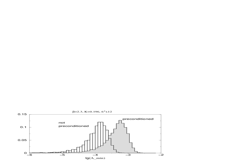
Figure 5: The distribution of the smallest eigenvalues of the squared preconditioned fermion matrix $\hat{Q}^{2}$ versus the non-preconditioned one $\tilde{Q}^{2}$ on a $6^{3}\cdot 12$ lattice at $\beta=2.3,K=0.196$.

The condition number and its fluctuations on different gauge configurations are dominated by the minimal eigenvalue. An example of a comparison of the fluctuations of the lowest eigenvalue of $\hat{Q}^{2}$ and $\tilde{Q}^{2}$ is shown in figure 5. As one sees, in this case the mean of the smallest eigenvalue becomes about a factor 4 larger due to preconditioning. At the same time the largest eigenvalue becomes smaller, therefore the average condition number becomes about a factor 5 smaller.

2.5 Parameter choice and autocorrelations

The two-step multi-bosonic algorithm has several algorithmic parameters which can be tuned to achieve optimal performance. In fact, our experience shows that this tuning can bring substantial gain in efficiency.

Polynomial degrees: In order to fix the polynomial degrees $n_{1\ldots 4}$, in practice one performs trial runs using increasing values. At the same time, by observing the range of eigenvalues, one also obtains the interval $[\epsilon,\lambda]$. The final value of $n_{1}$ is fixed by ensuring a high acceptance rate, around 90%, in the update correction step. $n_{2}$ has to be large enough to keep the measurement correction small in important physical quantities. The final precision of the updating is set by $n_{4}$, therefore the choice of $n_{1}$ and $n_{2}$ does not influence the expectation values. For showing a typical example, in the upper part of figure 6 the polynomial approximation $P_{n_{1}}^{(1)}$ and the product $P_{n_{1}}^{(1)}P_{n_{2}}^{(2)}$ are plotted in the interval $[\epsilon,\lambda]$. The product $P_{n_{1}}^{(1)}P_{n_{2}}^{(2)}P_{n_{4}}^{(4)}$ is displayed in the lower part of the figure. To the left (label a) the interval covers the range of the fluctuating smallest eigenvalue, whereas to the right (label b) the function is shown in the range of fluctuations of the last small eigenvalue which was determined explicitly. (In this case the correction factors were calculated from the eight smallest eigenvalues exactly and in the orthogonal subspace stochastically.)

To fix the degree of the third polynomial, $n_{3}$, we consider the probability $p_{1}$ of the system to jump between two identical configurations. In the limit $n_{3}\rightarrow\infty$ this probability tends obviously to 1. In practice $n_{3}$ is increased till we get $p_{1}\approx 0.99$, which is acceptable from the algorithm precision point of view, as one is convinced by comparing the expectation values. The choice of $n_{4}$ has to be tested, in principle, by observing its effect on the expectation values. Usually it is possible to choose already $n_{2}$ so large that the measurement corrections with a substantially higher $n_{4}$ are negligible compared with the statistical errors.

The parameters of the numerical simulations at $\beta=2.3$ are summarized in table 2. The runs with an asterisk had periodic boundary conditions for the gluino in the time direction $T$, the rest antiperiodic. $K$ is the hopping parameter and $[\epsilon,\lambda]$ is the interval of approximation for the first three polynomials of orders $n_{1,2,3}$, respectively. The fourth polynomial of order $n_{4}$ is defined on $[0,\lambda]$. In the last two columns the number of performed updating cycles, respectively, the number of parallelly updated lattices ($N_{lat}$) are given.

Table 2: Parameters of the numerical simulations at $\beta=2.3$. The notations are explained in the text.

lattice: $L,T$	$K$	$\epsilon$	$\lambda$	$n_{1}$	$n_{2}$	$n_{3}$	$n_{4}$	updates	$N_{lat}$
6,12∗	0.16	0.008	3.2	8	32	32	-	374400	64
6,12∗	0.17	0.008	3.2	8	32	32	-	332800	64
6,12∗	0.18	0.008	3.2	8	32	32	-	540800	64
6,12∗	0.185	0.002	3.4	12	32	48	-	384000	64
6,12	0.185	0.002	3.4	16	100	150	200	550400	64
6,12∗	0.19	0.0002	3.5	16	60	96	-	712800	64
6,12	0.19	0.0005	3.6	20	112	150	400	1487360	64
6,12∗	0.1925	0.00003	3.7	22	66	102	400	1280000	64
6,12	0.1925	0.0001	3.7	22	132	180	400	3655680	64
6,12∗	0.195	0.00003	3.7	22	66	102	400	1224000	64
6,12	0.195	0.00001	3.7	24	200	300	400	460800	64
6,12	0.196	0.00001	3.7	24	200	300	400	952320	64
6,12	0.1975	0.000001	3.8	30	300	400	500	506880	64
6,12	0.2	0.000001	3.9	30	300	400	500	599040	64
8,16	0.19	0.00065	3.55	20	82	112	-	1038400	32
8,16	0.1925	0.0001	3.6	22	142	190	-	870400	32
12,24	0.1925	0.0003	3.7	32	150	220	400	216000	9

Optimal ordering of the roots: The roots of $P_{n_{1}}^{(1)}$ have to be always calculated. As discussed in section 2.1, depending on the way of doing the global accept-reject in updating, sometimes the roots of $P_{n_{2}}^{(2)}$ are also needed. Concerning this point a non-trivial question is how to order the roots when the representation (14) is used. Choosing this order naively leads to overflow and underflow problems because the product in (14) involves in general very different orders of magnitude. A good solution [17] is minimizing the maximal ratio of the values $x^{\alpha}P_{p}(x)$ for $x\in[\epsilon,\lambda]$, where $P_{p}(x)$ denotes the partial product under consideration. This is in practice achieved by considering a discrete number of points in the interval $\{x_{1},\ldots,x_{N}\}$ where $N={\cal O}(n)$. This gives in general sufficient numerical stability even for orders of many hundreds (see also the tests performed in [23]).

Autocorrelations: During our simulations autocorrelations of different quantities were determined. Here we report on the analysis for the $12^{3}\cdot 24$ lattice at $\beta=2.3,K=0.1925$. Results for the $6^{3}\cdot 12$ and the $8^{3}\cdot 16$ lattices can be found in [3, 13]. We considered the short range exponential autocorrelation $\tau_{exp}$ of three different quantities, namely

• the $a$-$\eta^{\prime}$ propagator

• the gluino-glue propagator

• the plaquette

In the last case the data has been sufficient to give also an estimate of the integrated autocorrelation.

We started the analysis by calculating the autocorrelation function $C(t)$ for all these quantities. In case of the $a$-$\eta^{\prime}$ we calculated the autocorrelation of the propagator at time distance $\Delta t=1$, considering every 150’th configuration of the updating series. This was done separately on each of the lattices run in parallel. By averaging over the correlation functions obtained in this way we observed that the mean correlation function $\bar{C}^{a-\eta^{\prime}}(t)$ was at $t=1$ already compatible with zero ($\bar{C}^{a-\eta^{\prime}}(1)=0.028(19)$), which lead to the conclusion that $\tau^{a-\eta^{\prime}}_{exp}\leq 150$ updates.

Estimating the exponential autocorrelation $\tau_{exp}$ of the gluino-glue propagator we proceeded similarly as in the $a$-$\eta^{\prime}$ case. On all nine lattices that were run in parallel we determined independently the autocorrelation of the propagator at time distance $\Delta t=1$ on every 150’th configuration of our total history. The exponential autocorrelation time was then estimated by fitting an exponential of the form $\exp(-t/\tau_{exp})$ to the first points of the curve for each lattice. A typical autocorrelation function with the exponential fit can be seen in figure 7. By finally taking the average of $\tau_{exp}$ over all lattices we arrived at the result displayed in table 3. It has to be understood that $\tau_{exp}$ determined in this way displays a mode between the true short range exponential and the integrated autocorrelation, since only every 150’th sweep has been considered.

To estimate the integrated autocorrelation time $\tau_{int}$ of the plaquette we proceeded in a different manner. On the basis of prior analysis [3, 13] we expect the order of magnitude of $\tau_{int}$ to be $10^{2}\sim 10^{3}$. Since for each lattice we have a total of about $24000$ configurations in equilibrium we expect our time history to have a length of at most $\sim 100\tau_{int}$. This leads to the conclusion that standard methods to determine $\tau_{int}$ [24, 25] are not reliable since they require statistics that are at least of the order of several hundred $\tau_{int}$. Therefore, to estimate the order of magnitude of $\tau_{int}$ we proceed as follows. For each lattice run in parallel we calculated the autocorrelation function $C^{plaq}(t)$ of the plaquette for the complete history of $24000$ configurations. We fitted an exponential decay to $C^{plaq}(t)$ in a small interval (typically $[0,300]$) at the beginning where the fastest decay mode should be dominant. For longer distance the exponential typically decayed faster than $C^{plaq}(t)$. This expected behaviour could usually be observed up to a point $\hat{t}$ where $C^{plaq}(t)$ started to be dominated by its noise. We then calculated

$$\sum_{t=1}^{\hat{t}}C^{plaq}(t)$$ (41)

and took this value as an estimate of $\tau_{int}$. We expect this procedure only to lead to an order of magnitude estimate for the integrated autocorrelation. The typical behaviour for the autocorrelation function of the plaquette together with the exponential fit can be observed in figure 8. In this example the cutoff $\hat{t}$ has been chosen at about $\hat{t}\sim 3500$ updates since at this point $C^{plaq}(t)$ is clearly dominated by its noise. The final result for $\tau_{exp}$ and $\tau_{int}$ have been obtained by averaging over all nine lattices run in parallel, and can be found in table 3.

Table 3: Autocorrelation and integrated autocorrelation of the propagators and the plaquette on $12^{3}\cdot 24$ lattice at $\beta=2.3$ and $K=0.1925$.

	$\tau_{exp}$	$\tau_{int}$
$a$-$\eta^{\prime}$	$\leq 150$	-
gluino-glue	620(60)	1100(200)
plaquette	378(37)	675(43)

3 Confinement potential

The potential between static colour sources in gauge field theory is a physically very interesting quantity because it is characteristic for the dynamics of the gauge fields. If the sources are in the fundamental representation of the gauge group they can be called static quarks.

For a model containing dynamical matter fields in the fundamental representation, as is the case for QCD with dynamical quarks, they will screen the static quarks. The potential then approaches a constant at large distances [26]. The string tension $\sigma$, which is the asymptotic slope of the potential for large distances, vanishes accordingly. This type of screening is of a more kinematical nature.

On the other hand, if only matter fields in the adjoint representation of the gauge group are present, as in the case of supersymmetric N=1 Yang-Mills theory, there are different possibilities. Either the string tension does not vanish and static quarks are confined, or the static quarks are screened dynamically by the gauge fields. The latter situation is found in two-dimensional supersymmetric Yang-Mills theory [27]. The screening mechanism is related to the chiral anomaly and appears to be specific to two dimensions.

Four-dimensional SUSY Yang-Mills theory is believed to confine static quarks [28]. Furthermore, the behaviour of the string tension as a function of the gluino mass can give indications on the question, whether QCD and Super-QCD are smoothly linked [29].

We have determined the static quark potential and the string tension for N=1 SUSY Yang-Mills theory from our Monte Carlo results. The starting point are expectation values of rectangular Wilson loops $\langle W(R,T)\rangle$. In order to improve the overlap with the relevant ground state we have applied APE-smearing [30] to the Wilson loops. The optimal smearing radius turns out to be near $R_{s}=3$.

From the Wilson loops the potential can be found via

$$V(R)=\lim_{T\to\infty}V(R,T)\ ,$$ (42)

where

$$V(R,T)=\log\langle W(R,T)\rangle-\log\langle W(R,T+1)\rangle\ .$$ (43)

The large $T$ limit is approached exponentially [31]. We have obtained the potential $V(R)$ through a fit of the form

$$V(R,T)=V(R)+c_{1}(R)e^{-c_{2}(R)T}.$$ (44)

As an example we show $V(3,T)$ as a function of $T$ on a $12^{3}\cdot 24$ lattice in figure 9. For $T>6$ the errors grow significantly and we have chosen $1\leq T\leq 6$ as the best fit interval on this lattice. On the $8^{3}\cdot 16$ lattice fit intervals from $T=1$ to 4 or 5 yield consistent results.

In this way the static potential $V(R)$ has been obtained for $1\leq R\leq 6$ on the $8^{3}\cdot 16$ lattice and for $1\leq R\leq 9$ on the $12^{3}\cdot 24$ lattice. For larger values of $R$ the errors become rather large and the results are not reliable anymore. Anyhow, for $R>L/2$ increasing finite size effects are to be expected. In figures 10 and 11 the potential is shown on the $L=8$ lattice at $K=0.19$ and $L=12$ lattice at $K=0.1925$, respectively.

The string tension $\sigma$ is finally obtained by fitting the potential according to

$$V(R)=V_{0}-\frac{\alpha}{R}+\sigma R.$$ (45)

The value of $\sigma$ depends on the range of $R$ taken for the fit. In general it tends to decrease if the largest values of $R$ are included in the fit. However, this should not be interpreted as a signal for screening, since the potential is expected to bend down due to finite size effects. In table 4 the values for $\sqrt{\sigma}$ in lattice units are shown for different fit ranges.

Table 4: Square root of the string tension $\sigma$ in lattice units and Coulomb strength $\alpha$ from fits to $V(R)=V_{0}-\frac{\alpha}{R}+\sigma R$ over different ranges of $R$.

lattice	$K$	$R$ fit range	$a\sqrt{\sigma}$	$\alpha$
$8^{3}\cdot 16$	0.19	1 – 4	0.22(1)	0.23(2)
$8^{3}\cdot 16$	0.19	1 – 5	0.21(1)	0.25(1)
$8^{3}\cdot 16$	0.1925	1 – 4	0.21(1)	0.23(2)
$8^{3}\cdot 16$	0.1925	1 – 5	0.19(1)	0.25(2)
$12^{3}\cdot 24$	0.1925	1 – 6	0.17(1)	0.25(2)
$12^{3}\cdot 24$	0.1925	1 – 7	0.16(1)	0.26(2)
$12^{3}\cdot 24$	0.1925	1 – 8	0.13(2)	0.31(4)

We consider the range $1\leq R\leq L/2$ as reliable and quote as final results for the string tension

$$a\sqrt{\sigma} = 0.22(1)\hskip 14.22636pt\mbox{for}\ K=0.1900,\ L=8,$$

$$a\sqrt{\sigma} = 0.21(1)\hskip 14.22636pt\mbox{for}\ K=0.1925,\ L=8,$$

$$a\sqrt{\sigma} = 0.17(1)\hskip 14.22636pt\mbox{for}\ K=0.1925,\ L=12.$$ (46)

The string tension in lattice units is decreasing when the critical line is approached, as it should be. This is mainly caused by the renormalization of the gauge coupling due to virtual gluino loop effects which are manifested by decreasing lattice spacing $a$. From a comparison of the $L=8$ and $L=12$ results one sees that finite size effects still appear to be sizable. This has to be expected because we have for the spatial lattice extension $L=12a$ the result $L\sqrt{\sigma}\simeq 2.1$. In QCD with $\sqrt{\sigma}\simeq 0.45\,GeV$ this would correspond to $L\simeq 1\,fm$. Although we are dealing with a different theory where finite size effects as a function of $L\sqrt{\sigma}$ are different, for a first orientation this estimate should be good enough.

The coefficient $\alpha$ of the Coulomb term is close to the universal Lüscher value of $\pi/12=0.26$ [32].

For the ratio of the scalar glueball mass $m(0^{+})$, to be discussed below, and the square root of the string tension we get

$$m(0^{+})/\sqrt{\sigma} = 3.4(7)\hskip 8.53581pt\mbox{for}\ K=0.1900,\ L=8,$$

$$m(0^{+})/\sqrt{\sigma} = 3.0(4)\hskip 8.53581pt\mbox{for}\ K=0.1925,\ L=8,$$

$$m(0^{+})/\sqrt{\sigma} = 3.1(7)\hskip 8.53581pt\mbox{for}\ K=0.1925,\ L=12.$$ (47)

The uncertainties are not very small, but the numbers are consistent with a constant independent of $K$ in this range. They are of the same order of magnitude but somewhat smaller than in pure SU(2) gauge theory [33], where at $\beta=2.5$ we have $m(0^{+})/\sqrt{\sigma}=3.6$–$3.8$, depending on the lattice size.

4 Light bound state masses

The non-vanishing string tension observed in the previous section is in accordance with the general expectation [1, 4] that the Yang-Mills theory with gluinos is confining. Therefore the asymptotic states are colour singlets, similarly to hadrons in QCD. The structure of the light hadron spectrum is closest to the (theoretical) case of QCD with a single flavour of quarks where the chiral symmetry is broken by the anomaly.

Since both gluons and gluinos transform according to the adjoint (here triplet) representation of the colour group, one can construct colour singlet interpolating fields from any number of gluons and gluinos if their total number is at least two. Experience in QCD suggests that the lightest states can be well represented by interpolating fields build out of a small number of constituents. Simple examples are the glueballs known from pure Yang-Mills theory and gluinoballs corresponding to pseudoscalar mesons. We shall call the simplest pseudoscalar gluinoball made out of two gluinos the $a$-$\eta^{\prime}$ state. Here the label $a$ reminds us to the fact that the constituents are in the adjoint representation and $\eta^{\prime}$ stands for the corresponding $\eta^{\prime}$-meson in QCD. Mixed gluino-glueball states can be composed of any number of gluons and any number of gluinos, in the simplest case just one of both.

In general, one has to keep in mind that the classification of states by some interpolating fields has only a limited validity, because this is a strongly interacting theory where many interpolating fields can have important projections on the same state. Taking just the simplest colour singlets can, however, give a good qualitative description.

In the supersymmetric limit at zero gluino mass $m_{\tilde{g}}=0$ the hadronic states should occur in supermultiplets. This restricts the choice of simple interpolating field combinations and leads to low energy effective actions in terms of them [4, 5]. For non-zero gluino mass the supersymmetry is softly broken and the hadron masses are supposed to be analytic functions of $m_{\tilde{g}}$. The linear terms of a Taylor expansion in $m_{\tilde{g}}$ are often determined by the symmetries of the low energy effective actions [6].

The effective action of Veneziano and Yankielowicz [4] describes a chiral supermultiplet consisting of the $0^{-}$ gluinoball $a$-$\eta^{\prime}$, the $0^{+}$ gluinoball $a$-$f_{0}$, and a spin $\frac{1}{2}$ gluino-glueball. There is, however, no a priori reason to assume that glueball states are heavier than the members of the supermultiplet above. Therefore Farrar, Gabadadze and Schwetz [5] proposed an effective action which includes an additional chiral supermultiplet. This multiplet consists of a $0^{+}$ glueball, a $0^{-}$ glueball and another gluino-glueball. The effective action allows mass mixing between the members of the two supermultiplets. The masses of the lightest bound states and the mixing among them can be investigated by Monte Carlo simulations.

4.1 Glueballs

The glueball states as well as the methods to compute their masses in numerical Monte Carlo simulations are well known from pure gauge theory. (For a recent summary of results and references see [33].)

The lightest state is the $J^{P}=0^{+}$ glueball which can be generated by the symmetric combination of space-like plaquettes touching a lattice point. In order to optimize the signal and enhance the weight of the lightest state one is taking blocked [34] or smeared [30] links instead of the original ones. In order to obtain the masses, for a first orientation, one can use effective masses $m(t_{1},t_{2},T)$ assuming the dominance of a single state for time-slices $t_{1},t_{2}$ on the periodic lattice with time extension $T$. One can search for time distance intervals where the effective masses are roughly constant and then try single mass fits in these intervals. In cases with high enough statistics and corresponding small statistical errors two-mass fits in larger intervals can also be stable and give information on the mass of the next excited state.

Since no previous results on the glueball mass spectrum with dynamical gluinos are available in the literature, we started our search for dynamical gluino effects on small lattices as $4^{3}\cdot 8$ at hopping parameter values $K\geq 0.16$. We observed some effects for $K\geq 0.18$ where we started runs on larger lattices, up to $12^{3}\cdot 24$. As already seen in the previous section, the lattice spacing $a$ is decreasing with increasing $K$ (i.e. decreasing gluino mass). This means that effectively we are closer to the continuum limit at larger $K$, resulting in smaller glueball (and other) masses in lattice units. This effect is strongest at zero gluino mass where a first order phase transition is expected due to the discrete chiral symmetry breaking. First numerical evidence for this phase transition has been reported by our collaboration at $K=K_{0}=0.1955(5)$ [3].

With our spectrum calculations we stayed below this value and stopped at $K=0.1925$ where the $12^{3}\cdot 24$ lattice is already not very large. The obtained masses for the $0^{+}$ glueball in lattice units are

$$am(0^{+}) = 0.95(10)\hskip 8.53581pt\mbox{for}\ K=0.1800,\ L=6,$$

$$am(0^{+}) = 0.85(6)\hskip 14.22636pt\mbox{for}\ K=0.1850,\ L=6,$$

$$am(0^{+}) = 0.75(6)\hskip 14.22636pt\mbox{for}\ K=0.1900,\ L=8,$$

$$am(0^{+}) = 0.63(5)\hskip 14.22636pt\mbox{for}\ K=0.1925,\ L=8,$$

$$am(0^{+}) = 0.53(10)\hskip 8.53581pt\mbox{for}\ K=0.1925,\ L=12.$$ (48)

In addition to the $J^{P}=0^{+}$ glueball we have studied the pseudoscalar $0^{-}$ glueball. In order to create a pseudoscalar glueball from the vacuum with an operator built from closed loops on the lattice, one needs loops which cannot be rotated into their mirror images. For gauge group SU(2) the traces of loop variables are real and do not distinguish the two orientations of loops. The smallest loops with the desired property are made of eight links. One possibility would be to take the simplest lattice version of Tr($\epsilon_{\mu\nu\rho\sigma}F^{\mu\nu}F^{\rho\sigma}$). However, it contains two orthogonal plaquettes and cannot be put into a single time-slice. Therefore we have chosen to take the loop $\mathcal{C}$ shown in figure 12 [35].

The time-slice operator for the pseudoscalar glueball is then given by

$$S(t)=\sum_{R}[{\rm Tr}\,U(\mathcal{C})-{\rm Tr}\,U(P\mathcal{C})]\ ,$$ (49)

where the sum is over all rotations $R$ in the cubic lattice group and $P\mathcal{C}$ is the mirror image of $\mathcal{C}$. As usual, APE-smearing has been applied to the links appearing in the loop.

The pseudoscalar glueball mass has been calculated from the time-slice correlation functions as an effective mass from distances 1 and 2 with optimized smearing radius. On the $6^{3}\cdot 12$ lattice a good smearing radius is obtained for $R_{s}=4$ or 5, and the numbers are very stable. On the $8^{3}\cdot 16$ lattice a clear plateau in the number of smearing steps could not be seen. Nevertheless, for a smearing radius between 5 and 8 we obtain rather stable results. The masses in lattice units are

$$am(0^{-}) = 1.5(3)\hskip 19.91692pt\mbox{for}\ K=0.1850,\ L=6,$$

$$am(0^{-}) = 1.45(10)\hskip 8.53581pt\mbox{for}\ K=0.1900,\ L=6,$$

$$am(0^{-}) = 1.3(1)\hskip 19.91692pt\mbox{for}\ K=0.1925,\ L=6,$$

$$am(0^{-}) = 1.1(1)\hskip 19.91692pt\mbox{for}\ K=0.1925,\ L=8.$$ (50)

The pseudoscalar glueball appears to be roughly twice as heavy as the scalar one. This is similar to pure SU(2) gauge theory, where $m(0^{-})/m(0^{+})=1.8(2)$ [33].

4.2 Gluino-glueballs

One can construct colour singlet states from the gluinos and the field strength tensor in the adjoint representation. One of these states is a spin $\frac{1}{2}$ Majorana fermion which occurs in the construction of the Veneziano-Yankielowicz effective action [4]. In order to find the lowest mass in this channel we consider the correlator consisting of plaquettes connected by a quark propagator line:

$$\Gamma_{\tilde{g}g}(x,y)={\rm Tr_{spinor}}\,(\chi^{r}_{x}Q^{-1}_{xr,ys}\chi^{s}_{y})$$ (51)

where

$$\chi_{x}^{r}=\frac{1}{2i}{\rm Tr_{colour}}\,(\tau_{r}\bar{U}_{x})$$ (52)

and the plaquette variable is defined as

$$\bar{U}_{x}=U_{pl}(x,12)+U_{pl}(x,13)+U_{pl}(x,23)\ .$$ (53)

For antiperiodic boundary conditions for the gluino in the time direction the correlator is antiperiodic. By inserting $\gamma_{4}$ into the correlation function (51) it becomes periodic also with antiperiodic boundary conditions. The resulting projection on the ground state have in both cases either been compatible with one another, or the propagator modified with $\gamma_{4}$ has shown more mixing with larger masses. Therefore in extracting the masses we considered only the above propagator without $\gamma_{4}$.

For the gluino-glueball, in order to obtain a satisfactory signal, APE-smearing [30] has been implemented for the links and Jacobi-smearing [36] for the gluino field. Tests have shown [13] that Teper-blocking for the links was in this case not as well suited. Table 5 shows the smearing parameters used for the gluino-glueball on different lattices at different hopping parameters. They have been optimized by measuring the masses on a small sample of data and tuning the parameters accordingly to obtain the lowest mass values.

Table 5: Smearing parameters for Jacobi and APE-smearing used for measuring the gluino-glueball.

lattice	$K$	$N_{Jacobi}$	$K_{Jacobi}$	$N_{APE}$	$\epsilon_{APE}$
$8^{3}\cdot 16$	0.19	20	0.22	8	0.35
$8^{3}\cdot 16$	0.1925	23	0.185	12	0.34
$12^{3}\cdot 24$	0.1925	19	0.20	9	0.3

The masses for the gluino-glueball were determined first by considering effective masses $m(t_{1},t_{2},T)$ assuming the dominance of a single state for time-slices $t_{1},t_{2}$ on the periodic lattice with time extension $T$. From this time distance intervals were determined where the effective masses were roughly constant and single mass fits in these intervals were performed. The results are shown in table 6.

Table 6: Lowest masses for the gluino-glueball at different hopping parameters and lattices. The value of the gauge coupling has been $\beta=2.3$ throughout.

gluino-glueball	$K=0.18$	$K=0.185$	$K=0.19$	$K=0.1925$
$6^{3}\cdot 12$	1.93(5)	1.39(8)	1.05(20)	-
$8^{3}\cdot 16$	-	-	0.87(13)	0.82(18)
$12^{3}\cdot 24$	-	-	-	0.93(8)

4.3 Gluinoballs

Besides the gluino-glueball in this work we consider also gluinoballs defined by a colourless combination of two gluino fields. The $a$-$\eta^{\prime}$ has spin-parity $0^{-}$ and the $a$-$f_{0}$ spin-parity $0^{+}$. In the simulations for $a$-$\eta^{\prime}$ and $a$-$f_{0}$, respectively, the wave functions $\bar{\Psi}\gamma_{5}\Psi$ and $\bar{\Psi}\Psi$ were used. These gluinoballs are contained in the Veneziano-Yankielowicz super-multiplet [4]. For the correlation function a straightforward calculation as in [15] with $\Gamma\in\{1,\gamma_{5}\}$ yields

$$\Gamma_{\tilde{g}\tilde{g}}(x,y)=\langle{\rm Tr_{sc}}\,\{\Gamma Q^{-1}_{xx}\}{\rm Tr_{sc}}\,\{\Gamma Q^{-1}_{yy}\}-2\,{\rm Tr_{sc}}\,\{\Gamma Q^{-1}_{xy}\Gamma Q^{-1}_{yx}\}\rangle\ .$$ (54)

Note the factor of two originating from the Majorana character of the gluinos. In analogy with a flavour singlet meson in QCD the propagator consists of a connected and a disconnected part: the left, respectively, the right term of (54).

The numerical evaluation of the time-slice of the connected part can be reduced to the calculation of the propagator from a few initial points. The disconnected part is calculated using the volume source technique [37]. For the determination of the gluinoball propagator no smearing has been used.

In case of the $a$-$f_{0}$ particle the disconnected and the connected parts are of the same order of magnitude. The former has a much worse signal to noise ratio than the latter. This leads to a larger error on the $a$-$f_{0}$ as compared to the $a$-$\eta^{\prime}$ which is dominated by the connected part.

Our results for the $a$-$\eta^{\prime}$ and the $a$-$f_{0}$ masses for different lattices and hopping parameters can be found in table 7.

Table 7: Lowest masses for the $a$-$\eta^{\prime}$ and the $a$-$f_{0}$ at different hopping parameters and lattices. The gauge coupling is given by $\beta=2.3$ throughout. In the last column with a star the next higher mass is shown, whenever it could be determined.

$a$-$\eta^{\prime}$	$K=0.18$	$K=0.185$	$K=0.19$	$K=0.1925$	$K=0.1925^{*}$
$6^{3}\cdot 12$	1.155(11)	0.941(8)	0.594(14)	-	-
$8^{3}\cdot 16$	-	-	0.725(20)	0.551(17)	1.282(26)
$12^{3}\cdot 24$	-	-	-	0.48(5)	1.09(5)
$a$-$f_{0}$	$K=0.18$	$K=0.185$	$K=0.19$	$K=0.1925$	-
$6^{3}\cdot 12$	1.49(13)	1.11(17)	-	-
$8^{3}\cdot 16$	-	-	1.20(22)	0.81(17)
$12^{3}\cdot 24$	-	-	-	1.00(13)

In case of the $a$-$\eta^{\prime}$ the data has been good enough to estimate also the next higher state. (These data can be found in the column denoted by a star.) The lowest masses have been obtained by using effective masses and fits as for the gluino-glueball. The fits were rather stable in case of the $a$-$\eta^{\prime}$ on the $12^{3}\cdot 24$ lattice. This allowed to extract two masses from the data. Errors were estimated by the jackknife method.

4.4 Glueball-gluinoball mixing

In the low energy effective action of Farrar, Gabadadze and Schwetz [5] there is a possible non-zero mixing between the states in the two light supermultiplets. In particular there can be mixing of the $a$-$f_{0}$ gluinoball and the $0^{+}$ glueball.

In order to study the mixing we have calculated the connected cross-correlation functions

$$\Gamma_{ij}(t)=\langle S_{i}(t_{0})S_{j}(t_{0}+t)\rangle_{c}$$ (55)

where $i,j\in\{a,b\}$ and $S_{a}(t)$ is the plaquette operator creating a $0^{+}$ glueball from the vacuum, and $S_{b}(t)$ is the $\bar{\Psi}\Psi$ operator creating a $a$-$f_{0}$. If there is a non-zero mixing the hermitean correlation matrix $\Gamma_{ij}$ would not be diagonal. More generally one defines

$$\Lambda(t)=\left(\begin{array}[]{cc}\Gamma_{aa}(t)&\omega\Gamma_{ab}(t)\\ \omega\Gamma_{ba}(t)&\omega^{2}\Gamma_{bb}(t)\end{array}\right),$$ (56)

where $\omega$ is a real valued parameter. Diagonalizing $\Lambda(t)$ yields two eigenvalues, which are dominated by the lowest masses at large times $t$ [38]:

$$\lambda_{0}(t) = f_{0}(\omega)e^{-m_{0}t}\{1+O(e^{-(m_{1}-m_{0})t})\}$$ (57)

$$\lambda_{1}(t) = f_{1}(\omega)e^{-m_{1}t}\{1+O(e^{-\Delta m_{1}t})\},\hskip 8.53581pt\Delta m_{1}=\min(m_{1}-m_{0},m_{2}-m_{1}).$$ (58)

By tuning $\omega$ the statistical errors can be minimized. The masses $m_{0}$ and $m_{1}$ belong to the two lightest physical states in this channel. The mixing angle $\theta(t)$ is defined to be the angle between the eigenvector $v_{0}(t)$ corresponding to $\lambda_{0}$ and the vector $(1,0)$. For large $t$ one should observe a plateau where the mixing angle is constant and independent of $\omega$.

We have determined the mixing angle in the $0^{+}$ channel from our Monte Carlo data. If $\omega$ takes its optimal value $\omega_{0}=\sqrt{\Gamma_{aa}/\Gamma_{bb}}$ [36], the errors are smallest. Figure 13 shows the mixing angle $\theta(t)$ for this choice of $\omega$. On the $8^{3}\cdot 16$ lattice for $K=0.19$ and $K=0.1925$ as well as on the $12^{3}\cdot 24$ lattice for $K=0.1925$ the result is consistent with zero within rather small errors. So there is no mixing between the glueball and the $a$-$f_{0}$ state. It might be possible that mixing only becomes visible in the close vicinity of the critical line corresponding to zero gluino mass, where supersymmetry is nearly restored. On the other hand, the effective action of [5] does not necessarily require a non-zero mixing to be present.

5 Summary and outlook

The numerical Monte Carlo simulations presented in [3] and this paper are the first calculations of this kind in a Yang-Mills theory with light gluinos. Therefore an essential part of our work had to be invested in algorithmic studies and parameter tuning.

The two-step multi-bosonic algorithm, after appropriate tuning, turned out to be reliable and showed a satisfactory performance in the present case which is described by a flavour number $N_{f}=\frac{1}{2}$ of fermions in the adjoint representation. We showed that the sign of the Pfaffian appearing in a path integral formulation of gluinos can be taken into account, but does not practically influence the results in the investigated range of parameters. Since the two-step multi-bosonic algorithm can also be applied for any number of fermion flavours in the fundamental representation, an interesting physical application would be, for instance, QCD with three light flavours of quarks. On the basis of our positive experience with the algorithm we expect that it would also work well in that case.

Concerning parameter tuning in the lattice action, the problem is to find a region of bare parameter space where the gluino is light and where the lattice spacing is appropriate for feasible numerical simulations. Our strategy was to start at the lower end of the approximate scaling region in pure SU(2) lattice gauge theory at $\beta=2.3$ and to increase the hopping parameter $K$ as long as substantial effects of virtual dynamical gluino loops appear. It is expected that these effects decrease the lattice spacing due to the difference of the Callan-Symanzik $\beta$-functions with and without light gluinos. The observed effect is mainly an overall renormalization of $a$. The change of dimensionless ratios of masses and string tension are only moderate up to $K\leq 0.1925$, where most of our simulations were performed.

Increasing $K$ further is getting more difficult from the algorithmic point of view because the smallest eigenvalues of the fermion matrix are becoming really small. In spite of this our algorithm still performed reasonably well. A search in the range up to $K\leq 0.20$ revealed first evidence for a first order phase transition expected to occur at zero gluino mass [3]. Our present estimate for the location of this phase transition, at $\beta=2.3$, is $K_{0}=0.1955(5)$. This gives for the bare gluino mass in lattice units

$$am_{0}\equiv\frac{1}{2}\left[\frac{1}{K}-\frac{1}{K_{0}}\right]$$ (59)

a value $am_{0}\simeq 0.04$ at $K=0.1925$. With the value of the string tension in (3) we get $m_{0}/\sqrt{\sigma}\simeq 0.2$. Using QCD-units and neglecting the mass renormalization factor $Z_{m}$ of the order of 1 this corresponds to a light gluino mass of about $100\,MeV$. Of course, this can only serve as an order of magnitude guide because SYM and QCD are after all two different theories. In order to connect $m_{0}$ to, say, $\Lambda_{\overline{MS}}$ one had to perform a calculation as in [39] with massless gluinos.

Table 8: Masses of the light bound states at $\beta=2.3$ in lattice units.

lattice: $L,T$	$K$	$am^{0^{+}}_{gg}$	$am^{0^{-}}_{gg}$	$am^{0^{+}}_{\tilde{g}\tilde{g}}$	$am^{0^{-}}_{\tilde{g}\tilde{g}}$	$am_{\tilde{g}g}$
6,12	0.18	0.95(10)	-	1.49(13)	1.155(11)	1.93(5)
6,12	0.185	0.85(6)	1.5(3)	1.11(17)	0.941(8)	1.39(8)
8,16	0.19	0.75(6)	-	1.20(22)	0.725(20)	0.87(13)
8,16	0.1925	0.63(5)	1.1(1)	0.81(17)	0.551(17)	0.82(18)
12,24	0.1925	0.53(10)	-	1.00(13)	0.48(5)	0.93(8)

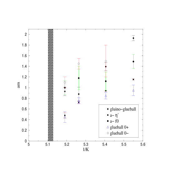
Figure 14: The lightest bound state masses in lattice units as function of the bare gluino mass parameter $1/K$. The shaded area at $K=0.1955(5)$ is where zero gluino mass and supersymmetry are expected.

Having an algorithm and knowing the interesting range of parameters in the lattice action one can start to perform numerical simulations for determining the spectrum of states and other physically interesting features. The properties of the lightest states are obviously quite interesting because the construction of low energy effective actions [4, 5] is based on the assumptions about the relevant composite field variables. An important constraint on the spectrum is that in the limit of zero gluino mass, where supersymmetry is expected, the particle states should occur in supermultiplets with degenerate mass. A collection of our present results on the lightest states is displayed in table 8 and figure 14.

As one can see, for the lightest gluino masses (highest hopping parameters $K$) the bound state masses can be arranged into two groups. The lightest states are the $0^{-}$ gluinoball ($a$-$\eta^{\prime}$) and the $0^{+}$ glueball. At $K=0.1925$ these are in lattice units both near $am\simeq 0.5$. The other group of states is at $K=0.1925$ near $am\simeq 1.0$ and consists of the $0^{+}$ gluinoball, the $0^{-}$ glueball and the spin-$\frac{1}{2}$ gluino-glueball. As shown by figure 13, there is practically no mixing between the $0^{+}$-states in the two groups. The disturbing fact concerning supersymmetry is that there is apparently no spin-$\frac{1}{2}$ state in the lower mass group. We saw this problem already at early stages of our project and hence paid specific attention to a lighter spin-$\frac{1}{2}$ gluino-glueball state, but we did not find it.

There are several possible explanations for this. Perhaps we are not yet close enough to the supersymmetric limit and therefore the spectrum does not yet look like a weakly broken supersymmetric spectrum. Another possibility is that we are missing the other spin-$\frac{1}{2}$ state because our choice of interpolating fields is not appropriate. One can, for instance, think about spin-$\frac{1}{2}$ gluinoballs made out of three gluinos which appear at strong coupling [40] and were not exploited in our simulations. Nevertheless, even if the spin-$\frac{1}{2}$ state completing the lightest supermultiplet would be dominated by three gluinos, the emerging structure of the two light supermultiplets would be surprising. Finally one can think about possible finite volume effects and the effect of lattice artifacts breaking supersymmetry at finite lattice spacing. Without further numerical simulations we cannot exclude this last possibility but we believe that it is unlikely on basis of the experience in pure gauge theories. The product of the lattice spacing with the square-root of the string tension is at $K=0.1925$ given by $a\sqrt{\sigma}\simeq 0.17$. In pure SU(2) gauge theory [33] we have a similar value at $\beta\simeq 2.5-2.6$ which is within the region of reasonably good scaling. As discussed in section 3, the spatial volume extension of our $12^{3}$ lattice at $K=0.1925$ is about $1\,fm$ in QCD units. This is almost certainly not large enough and therefore there are important finite volume effects to be expected, but the qualitative features of the bound state spectrum should already be visible in such volumes.

We leave this puzzle for further investigations. The most important outcome of this first Super-Yang-Mills simulation with light gluinos is that the numerical Monte Carlo calculations are definitely possible with present-day techniques and can certainly contribute to the better understanding of the low energy non-perturbative dynamics of supersymmetric gauge theories.

Acknowledgement: The numerical simulations presented here have been performed on the CRAY-T3E computers at John von Neumann Institute for Computing (NIC), Jülich. We thank NIC and the staff at ZAM for their kind support.

Appendix

Appendix A Least-squares optimized polynomials

Least-squares optimization provides a general and flexible framework for obtaining the necessary optimized polynomials in multi-bosonic fermion algorithms. By exploiting different weight functions this framework is well suited to fulfill rather different requirements.

In the first part of this appendix the basic formulae from [17] are collected. In the second part a simple example is considered: in case of an appropriately chosen weight function the least-squares optimized polynomials for the approximation of the function $x^{-\alpha}$ are expressed in terms of Jacobi polynomials.

A.1 Definition and basic relations

The general theory of least-squares optimized polynomial approximations can be inferred from the literature [41, 42]. Here we introduce the basic formulae in the way it has been done in [17] for the specific needs of multi-bosonic fermion algorithms. We shall keep the notations there, apart from a few changes which allow for more generality.

We want to approximate the real function $f(x)$ in the interval $x\in[\epsilon,\lambda]$ by a polynomial $P_{n}(x)$ of degree $n$. The aim is to minimize the deviation norm

$$\delta_{n}\equiv\left\{N_{\epsilon,\lambda}^{-1}\;\int_{\epsilon}^{\lambda}dx\,w(x)^{2}\left[f(x)-P_{n}(x)\right]^{2}\right\}^{\frac{1}{2}}\ .$$ (60)

Here $w(x)$ is an arbitrary real weight function and the overall normalization factor $N_{\epsilon,\lambda}$ can be chosen by convenience, for instance, as

$$N_{\epsilon,\lambda}\equiv\int_{\epsilon}^{\lambda}dx\,w(x)^{2}f(x)^{2}\ .$$ (61)

A typical example of functions to be approximated is $f(x)=x^{-\alpha}/\bar{P}(x)$ with $\alpha>0$ and some polynomial $\bar{P}(x)$. The interval is usually such that $0\leq\epsilon<\lambda$. For optimizing the relative deviation one takes a weight function $w(x)=f(x)^{-1}$.

It turns out useful to introduce orthogonal polynomials $\Phi_{\mu}(x)\;(\mu=0,1,2,\ldots)$ satisfying

$$\int_{\epsilon}^{\lambda}dx\,w(x)^{2}\Phi_{\mu}(x)\Phi_{\nu}(x)=\delta_{\mu\nu}q_{\nu}\ .$$ (62)

and expand the polynomial $P_{n}(x)$ in terms of them:

$$P_{n}(x)=\sum_{\nu=0}^{n}d_{n\nu}\Phi_{\nu}(x)\ .$$ (63)

Besides the normalization factor $q_{\nu}$ let us also introduce, for later purposes, the integrals $p_{\nu}$ and $s_{\nu}$ by

$$q_{\nu}\equiv\int_{\epsilon}^{\lambda}dx\,w(x)^{2}\Phi_{\nu}(x)^{2}\ ,\hskip 20.00003ptp_{\nu}\equiv\int_{\epsilon}^{\lambda}dx\,w(x)^{2}\Phi_{\nu}(x)^{2}x\ ,\hskip 20.00003pts_{\nu}\equiv\int_{\epsilon}^{\lambda}dx\,w(x)^{2}x^{\nu}\ .$$ (64)

It can be easily shown that the expansion coefficients $d_{n\nu}$ minimizing $\delta_{n}$ are independent of $n$ and are given by

$$d_{n\nu}\equiv d_{\nu}=\frac{b_{\nu}}{q_{\nu}}\ ,$$ (65)

where

$$b_{\nu}\equiv\int_{\epsilon}^{\lambda}dx\,w(x)^{2}f(x)\Phi_{\nu}(x)\ .$$ (66)

The minimal value of $\delta_{n}^{2}$ is

$$\delta_{n}^{2}=1-N_{\epsilon,\lambda}^{-1}\sum_{\nu=0}^{n}d_{\nu}b_{\nu}\ .$$ (67)

The above orthogonal polynomials satisfy three-term recurrence relations which are very useful for numerical evaluation. The first two of them with $\mu=0,1$ are given by

$$\Phi_{0}(x)=1\ ,\hskip 20.00003pt\Phi_{1}(x)=x-\frac{s_{1}}{s_{0}}\ .$$ (68)

The higher order polynomials $\Phi_{\mu}(x)$ for $\mu=2,3,\ldots$ can be obtained from the recurrence relation

$$\Phi_{\mu+1}(x)=(x+\beta_{\mu})\Phi_{\mu}(x)+\gamma_{\mu-1}\Phi_{\mu-1}(x)\ ,\hskip 20.00003pt(\mu=1,2,\ldots)\ ,$$ (69)

where the recurrence coefficients are given by

$$\beta_{\mu}=-\frac{p_{\mu}}{q_{\mu}}\ ,\hskip 30.00005pt\gamma_{\mu-1}=-\frac{q_{\mu}}{q_{\mu-1}}\ .$$ (70)

Using these relations on can set up a recursive scheme for the computation of the orthogonal polynomials in terms of the basic integrals $s_{\nu}$ defined in (64). Defining the polynomial coefficients $f_{\mu\nu}\;(0\leq\nu\leq\mu)$ by

$$\Phi_{\mu}(x)=\sum_{\nu=0}^{\mu}f_{\mu\nu}x^{\mu-\nu}$$ (71)

the above recurrence relations imply the normalization convention

$$f_{\mu 0}=1\ ,\hskip 30.00005pt(\mu=0,1,2,\ldots)\ ,$$ (72)

and one can easily show that $q_{\mu}$ and $p_{\mu}$ satisfy

$$q_{\mu}=\sum_{\nu=0}^{\mu}f_{\mu\nu}s_{2\mu-\nu}\ ,\hskip 20.00003ptp_{\mu}=\sum_{\nu=0}^{\mu}f_{\mu\nu}\left(s_{2\mu+1-\nu}+f_{\mu 1}s_{2\mu-\nu}\right)\ .$$ (73)

The coefficients themselves can be calculated from $f_{11}=-s_{1}/s_{0}$ and (69) which gives

$$f_{\mu+1,1} = f_{\mu,1}+\beta_{\mu}\ ,$$

$$f_{\mu+1,2} = f_{\mu,2}+\beta_{\mu}f_{\mu,1}+\gamma_{\mu-1}\ ,$$

$$f_{\mu+1,3} = f_{\mu,3}+\beta_{\mu}f_{\mu,2}+\gamma_{\mu-1}f_{\mu-1,1}\ ,$$

$$\ldots$$

$$f_{\mu+1,\mu} = f_{\mu,\mu}+\beta_{\mu}f_{\mu,\mu-1}+\gamma_{\mu-1}f_{\mu-1,\mu-2}\ ,$$

$$f_{\mu+1,\mu+1} = \beta_{\mu}f_{\mu,\mu}+\gamma_{\mu-1}f_{\mu-1,\mu-1}\ .$$ (74)

The polynomial and recurrence coefficients are recursively determined by (72)-(A.1). The expansion coefficients for the optimized polynomial $P_{n}(x)$ can be obtained from (65) and

$$b_{\mu}=\sum_{\nu=0}^{\mu}f_{\mu\nu}\int_{\epsilon}^{\lambda}dx\,w(x)^{2}f(x)x^{\mu-\nu}\ .$$ (75)

A.2 A simple example: Jacobi polynomials

The approximation interval $[\epsilon,\lambda]$ can be transformed to some standard interval, say, $[-1,1]$ by the linear mapping

$$\xi=\frac{2x-\lambda-\epsilon}{\lambda-\epsilon}\ ,\hskip 20.00003ptx=\frac{\xi}{2}(\lambda-\epsilon)+\frac{1}{2}(\lambda+\epsilon)\ .$$ (76)

A weight factor $(1+\xi)^{\rho}(1-\xi)^{\sigma}$ with $\rho,\sigma>-1$ corresponds in the original interval to the weight factor

$$w^{(\rho,\sigma)}(x)^{2}=(x-\epsilon)^{\rho}(\lambda-x)^{\sigma}\ .$$ (77)

Taking, for instance, $\rho=2\alpha,\;\sigma=0$ this weight is similar to the one for relative deviation from the function $f(x)=x^{-\alpha}$, which would be just $x^{2\alpha}$. In fact, for $\epsilon=0$ these are exactly the same and for small $\epsilon$ the difference is negligible. The advantage of considering the weight factor in (77) is that the corresponding orthogonal polynomials are simply related to the Jacobi polynomials [43, 44], namely

$$\Phi^{(\rho,\sigma)}_{\nu}(x)=(\lambda-\epsilon)^{\nu}\nu!\,\frac{\Gamma(\rho+\sigma+\nu+1)}{\Gamma(\rho+\sigma+2\nu+1)}P^{(\sigma,\rho)}_{\nu}\left(\frac{2x-\lambda-\epsilon}{\lambda-\epsilon}\right)\ .$$ (78)

Our normalization convention (72) implies that

$$q^{(\rho,\sigma)}_{\nu}=(\lambda-\epsilon)^{\rho+\sigma+2\nu+1}\nu!\,\frac{\Gamma(\rho+\nu+1)\Gamma(\sigma+\nu+1)\Gamma(\rho+\sigma+\nu+1)}{\Gamma(\rho+\sigma+2\nu+1)\Gamma(\rho+\sigma+2\nu+2)}\ .$$ (79)

The coefficients of the orthogonal polynomials are now given by

$$f^{(\rho,\sigma)}_{\mu\nu}=\sum_{\omega=0}^{\nu}(-\epsilon)^{\nu-\omega}(\epsilon-\lambda)^{\omega}\left(\begin{array}[]{c}\mu-\omega\\ \nu-\omega\end{array}\right)\left(\begin{array}[]{c}\mu\\ \omega\end{array}\right)\frac{\Gamma(\rho+\mu+1)\Gamma(\rho+\sigma+2\mu-\omega+1)}{\Gamma(\rho+\mu-\omega+1)\Gamma(\rho+\sigma+2\mu+1)}\ .$$ (80)

In particular, we have

$$f^{(\rho,\sigma)}_{\mu 0}=1\ ,\hskip 20.00003ptf^{(\rho,\sigma)}_{11}=-\epsilon-(\lambda-\epsilon)\frac{(\rho+1)}{(\rho+\sigma+2)}\ .$$ (81)

The coefficients $\beta,\gamma$ in the recurrence relation (69) can be derived from the known recurrence relations of the Jacobi polynomials:

$$\beta^{(\rho,\sigma)}_{\mu}=-\frac{1}{2}(\lambda+\epsilon)+\frac{(\sigma^{2}-\rho^{2})(\lambda-\epsilon)}{2(\rho+\sigma+2\mu)(\rho+\sigma+2\mu+2)}\ ,$$

$$\gamma^{(\rho,\sigma)}_{\mu-1}=-(\lambda-\epsilon)^{2}\,\frac{\mu(\rho+\mu)(\sigma+\mu)(\rho+\sigma+\mu)}{(\rho+\sigma+2\mu-1)(\rho+\sigma+2\mu)^{2}(\rho+\sigma+2\mu+1)}\ .$$ (82)

In order to obtain the expansion coefficients of the least-squares optimized polynomials one has to perform the integrals in (75). As an example, let us consider the function $f(x)=x^{-\alpha}$ when the necessary integrals can be expressed by hypergeometric functions:

$$\int_{\epsilon}^{\lambda}dx\,(x-\epsilon)^{\rho}(\lambda-x)^{\sigma}x^{\mu-\nu-\alpha}=$$

$$=(\lambda-\epsilon)^{\rho+\sigma+1}\lambda^{\mu-\nu-\alpha}\frac{\Gamma(\rho+1)\Gamma(\sigma+1)}{\Gamma(\rho+\sigma+2)}F\left(\alpha-\mu+\nu,\sigma+1;\rho+\sigma+2;1-\frac{\epsilon}{\lambda}\right)\ .$$ (83)

Let us now consider, for simplicity, only the case $\epsilon=0$, when we obtain

$$b^{(\rho,\sigma)}_{\mu}=(-1)^{\mu}\lambda^{1+\rho+\sigma+\mu-\alpha}\frac{\Gamma(\rho+\sigma+\mu+1)\Gamma(\alpha+\mu)\Gamma(\rho-\alpha+1)\Gamma(\sigma+\mu+1)}{\Gamma(\rho+\sigma+2\mu+1)\Gamma(\alpha)\Gamma(\rho+\sigma-\alpha+\mu+2)}\ .$$ (84)

Combined with (65) and (79) this leads to

$$d^{(\rho,\sigma)}_{\mu}=(-1)^{\mu}\lambda^{-\mu-\alpha}\frac{\Gamma(\rho+\sigma+2\mu+2)\Gamma(\alpha+\mu)\Gamma(\rho-\alpha+1)}{\mu!\,\Gamma(\rho+\mu+1)\Gamma(\alpha)\Gamma(\rho+\sigma-\alpha+\mu+2)}\ .$$ (85)

These formulae can be used, for instance, for fractional inversion. For the parameters $\rho,\sigma$ the natural choice in this case is $\rho=2\alpha,\sigma=0$ which corresponds to the optimization of the relative deviation from the function $f(x)=x^{-\alpha}$. As we have seen in section A.1, the optimized polynomials are the truncated expansions of $x^{-\alpha}$ in terms of the Jacobi polynomials $P^{(2\alpha,0)}$. The Gegenbauer polynomials proposed in [45] for fractional inversion correspond to a different choice, namely $\rho=\sigma=\alpha-\frac{1}{2}$. This is because of the relation

$$C^{\alpha}_{n}(x)=\frac{\Gamma(n+2\alpha)\Gamma(\alpha+\frac{1}{2})}{\Gamma(2\alpha)\Gamma(n+\alpha+\frac{1}{2})}P^{(\alpha-\frac{1}{2},\alpha-\frac{1}{2})}_{n}(x)\ .$$ (86)

Note that for the simple case $\alpha=1$ we have here the Chebyshev polynomials of second kind: $C^{1}_{n}(x)=U_{n}(x)$.

In our present application we have to consider $\alpha=\frac{1}{4}$. For the first polynomial $P^{(1)}_{n_{1}}$ we could, for instance, use the Gegenbauer polynomials $G^{\frac{1}{4}}$ corresponding to $P^{(-\frac{1}{4},-\frac{1}{4})}$. (For $P^{(2,3,4)}$ we need, of course, the polynomials introduced in [15] which approximate more complicated functions.) A numerical comparison shows, however, that the least squares optimized polynomials minimizing the relative deviation in the interval $[\epsilon,\lambda]$ are better than the Gegenbauer polynomials (see fig. 15): both approximations are similar at the lower end of the interval but otherwise the deviations of the former are by a factor of five smaller.

The special case $\alpha=\frac{1}{2}$ is interesting for the numerical evaluation of the zero mass lattice action proposed by Neuberger [46]. In this case, in order to obtain the least-squares optimized relative deviation with weight function $w(x)=x$, the function $x^{-\frac{1}{2}}$ has to be expanded in the Jacobi polynomials $P^{(1,0)}$. Note that this is different both from the Chebyshev and the Legendre expansions applied in [47]. The former would correspond to take $P^{(-\frac{1}{2},-\frac{1}{2})}$, the latter to $P^{(0,0)}$. The corresponding weight functions would be $[x(\lambda-x)]^{-\frac{1}{2}}$ and $1$, respectively. As a consequence of the divergence of the weight factor at $x=0$, the Chebyshev expansion is not appropriate for an approximation in an interval with $\epsilon=0$. This can be immediately seen from the divergence of $d^{(-\frac{1}{2},-\frac{1}{2})}_{\mu}$ at $\alpha=\frac{1}{2}$ in (85).

The advantage of the Jacobi polynomials appearing in these examples is that they are analytically known. The more general least-squares optimized polynomials defined in the previous subsection can also be numerically expanded in terms of them. This is sometimes more comfortable than the entirely numerical approach.

Appendix B Determining the smallest eigenvalues

For finding the smallest eigenvalues and the corresponding eigenvectors of the squared hermitean fermion matrix $\tilde{Q}^{2}=Q^{\dagger}Q$ we apply the algorithm of Kalkreuter and Simma [48]. Some modifications and the optimization with detailed tests have been described in [13]. Here we give a short summary for the readers convenience.

The smallest eigenvalue of a general hermitean matrix $H$ can be found by minimizing the Ritz functional

$$\mu_{H}(z)\equiv\frac{(z^{*}Hz)}{(z^{*}z)}\ .$$ (87)

Here the notation defined in (31) is used, with $z^{*}$ denoting the complex conjugate vector of $z$ and $(xy)\equiv(xIy)=(yx)$, where $I$ is the unit matrix. The gradient of the Ritz functional is obviously

$$g_{H}(z)=\frac{Hz(z^{*}z)-z(z^{*}Hz)}{(z^{*}z)^{2}}\ .$$ (88)

For the conjugate gradient procedure we can choose a starting search direction $p_{1}=-g_{H}(z)$ and the iteration is defined by a new approximation to the eigenvector

$$z_{i+1}=z_{i}+\alpha_{i}p_{i}\ ,\hskip 30.00005pti=1,2,\ldots\;\ .$$ (89)

The factor $\alpha_{i}$ is chosen at the minimum of $\mu_{H}(z)$ in the search direction $p_{i}$. One can show that

$$\alpha_{i}=\frac{2\,(p_{i}^{*}Hz_{i})}{(z_{i}^{*}Hz_{i})-(p_{i}^{*}Hp_{i})-\sqrt{[(z_{i}^{*}Hz_{i})-(p_{i}^{*}Hp_{i})]^{2}+4\,(p_{i}^{*}Hz_{i})(z_{i}^{*}Hp_{i})]}}\ .$$ (90)

Let us note that taking the positive sign in front of the square root gives the maximum, instead of the minimum. The other sign can be used for finding the maximal eigenvalue instead of the minimal one. In the iteration relation (89) the conjugate search direction $p_{i+1}$ can be chosen according to [48]

$$p_{i+1}=g_{H}(z_{i+1})+\beta_{i}\left[p_{i}-z_{i+1}\frac{(z^{*}_{i+1}p_{i})}{(z^{*}_{i+1}z_{i+1})}\right]\ .$$ (91)

For the factor $\beta_{i}$ one can take, according to the Fletcher-Reeves prescription, with $g_{i}\equiv g_{H}(z_{i})$

$$\beta_{i}=\frac{(g^{*}_{i+1}g_{i+1})}{(g^{*}_{i}g_{i})}$$ (92)

or alternatively, according to the Polak-Ribiere prescription,

$$\beta_{i}=\frac{(g^{*}_{i+1}g_{i+1})-(g^{*}_{i}g_{i+1})}{(g^{*}_{i}g_{i})}\ .$$ (93)

It turned out that in case of our fermion matrices the Polak-Ribiere version is 25% to 40% more efficient than the Fletcher-Reeves version proposed in [48]. In naive implementations of this iterative procedure numerical problems may occur due to the increasing length of the vector $z_{i}$. Since the Ritz functional is scale invariant, this problem can be avoided by rescaling, typically every 25 steps, as

$$z_{i}\to\frac{z_{i}}{\sqrt{(z_{i}^{*}z_{i})}}\ ,\hskip 20.00003ptp_{i}\to p_{i}\,\sqrt{(z_{i}^{*}z_{i})}\ ,\hskip 20.00003ptg_{i}\to g_{i}\,\sqrt{(z_{i}^{*}z_{i})}\ .$$ (94)

Several smallest eigenvalues might be determined by applying the above conjugate gradient iteration subsequently to the projection into the orthogonal subspaces defined by

$$H_{k}=P^{\perp}_{k}HP^{\perp}_{k}\ ,\hskip 20.00003ptP^{\perp}_{k}v\equiv v-\sum_{i=1}^{k-1}v_{i}\,(v_{i}^{*}v)\ ,\hskip 20.00003pt(k=2,3,\ldots)\ .$$ (95)

Here $v_{i}$ denote the previously found normalized eigenvectors. This naive procedure becomes numerically instable after a few eigenvalues because of the numerical errors in the projectors $P^{\perp}_{k}$. One can stabilize and speed up this sequential search if one embeds it in an iterative scheme [48]. If one is interested in the $k_{max}$ smallest eigenvalues then, after finding some approximation to $v_{1},v_{2},\ldots,v_{k_{max}}$ in a sequential search, the $k_{max}\otimes k_{max}$ matrix

$$M_{ij}\equiv(v_{i}^{*}Hv_{j})$$ (96)

is diagonalized. For reasonable values of $k_{max}$ this is a small problem and the resulting new eigenvalues and the corresponding eigenvectors

$$v^{\prime}_{i}=\sum_{j=1}^{k_{max}}\xi^{(i)}_{j}v_{j}$$ (97)

are better than $v_{i}$. Here $\xi^{(i)}$ denotes the eigenvectors of the matrix $M$. After this intermediate diagonalization the sequential search with conjugate gradient iterations is continued.

After the restarting of the sequential search it takes some time until the search directions of the conjugate gradient iterations become again optimal. Therefore it is not good to insert an intermediate diagonalization too often, especially at later stages when the final precision is approached. In our project a good performance could be achieved if between the $i$-th and $(i+1)$-th intermediate diagonalization the sequential search was performed with $(5+10i)$ conjugate gradient iterations. The application of the projectors $P^{\perp}_{k}$ becomes, even for moderate values of $k$, quite expensive. Since $P^{\perp}_{k}$ projects out approximate eigenspaces of $H$, it is not necessary to apply it at every conjugate gradient iteration. Tests show that it suffices to perform the projection only in the intermediate diagonalizations and, say, after every 25-th conjugate gradient iterations.

The optimization of the Kalkreuter-Simma algorithm pays off very well [13]. It turns out that the number of necessary conjugate gradient iterations per eigenvalue is getting smaller and smaller with increasing values of $k_{max}$. Another feature is that the last few of the $k_{max}$ eigenvalues are slowly converging. As a consequence, for computing more than $k_{max}=16$ eigenvalues, it is advantageous to run the algorithm with $k_{max}^{\prime}$, say, 5% larger than $k_{max}$ and stop the iteration if the smallest $k_{max}$ eigenvalues satisfy the stopping criterion.

Appendix C High performance C++ for LGT simulations

When starting to develop the software for the DESY-Münster Collaboration we decided to take care for the reusability and flexibility of the code. It is well known that object oriented design and programming (OOD, OOP) helps to fulfill these needs [49]. A widely spread prejudice against OOP is bad performance. But new techniques like expression templates [50, 51, 52] or temporary base class idiom [53] encouraged us to use an object oriented approach for the software development. There were serveral reasons, which led to the decision of using C++ in our project. It is the only object oriented (OO) language available for high performance computers and it is a high efficient OO language. Message Passing (MPI) and multithreading libraries (POSIX threads) are also usable with C++. With the help of templates C++ also supports generic programming [54]. This feature allows one, for instance, to write a code template for the whole lattice gauge theory (LGT) simulation without specifying the gauge group. By simply providing a gauge group class which describes the basic functionality of the desired gauge group (SU(2), SU(3) etc), the compiler is able to generate code. Generic programming made possible to port our Super-Yang-Mills simulation program from SU(2) to SU(3) in less than one week. The only thing we had to add was a high efficient SU(3) class which consisted of approximately 800 lines (less than $2\%$ of the project).

By using these techniques the efficiency of the simulation code stands and falls with an efficient vector class. A problem that arises almost always while overloading numerical operators of a vector class is the generation of temporary objects. This problem is not only limited to C++ but also to Fortran90. As a simple example let us consider

$$\vec{a}=\underbrace{\underbrace{\vec{x}+\vec{y}}_{\vec{t_{1}}}+\vec{z}}_{\vec{t_{2}}=\vec{t_{1}}+\vec{z}}\ .$$ (98)

$\vec{t_{1}}$ is generated in a function, which means on the stack. If the function is left this temporary object has to be copied away from the stack using the so called copy constructor. That means the copy constructor is used to generate a temporary copy from a temporary object. Furthermore the compiler may generate hidden temporary vectors using the copy constructor.

A popular method to avoid unnecessary copying is reference counting [55]. But due to the additional level of indirection reference counting is efficient only for large vectors and suited for typical vector length of dynamical fermion simulations. The basic ideas of two other solutions which are working fine for both, small and large vectors are

• Temporary Base Class Idiom

  • introduces an own class TmpVector for temporary vectors,

  • TmpVector construct/destructed shallowly,

  • operator+(Vector &) returns a TmpVector,

  • operator+(TmpVector) is implemented as TmpVector+=Vector,

  • disadvantage: four times more operators have to be overloaded.

• Expression Templates

  • avoids temporary objects in the first place by automatically transforming
    vector u,v,w; u=v+w; at compile time (more or less) into

       for (int i(0); i < u.length(); ++i)
       u[i]=v[i] + w[i];
      
    

    using template meta programming (or compile time programs).

On one hand it is desirable to implement a class for handling gamma matrices. On the other hand it is obvious that the gamma matrix multiplication has to be done at compile time rather than at run time. Otherwise a fermion matrix multiplication would proceed at a snail‘s pace. Two techniques exist to achieve this.

• Lazy Evaluation for $\mathbf{\gamma_{\mu}\psi}$

  • delays computation until the result is needed.

  • processes expressions like $\chi+\gamma_{\mu}\psi$ in a single task.

• Expression $\mathbf{\gamma_{\mu}\gamma_{\nu}}$

  • forces the compiler to perform this multiplication a compile time using template meta programming [56]

To test the efficiency of different vector classes we used a Monte-Carlo simulation of the two dimensional $\sigma$-model. This is a worst case test for a vector class because the vector length is three. The administration overhead caused by the introduction of a class can be huge compared to the performed operation. Generally the difference between the class libraries are small for larger vector sizes. As one can see in tabular (9) Blitz++ (Expression templates) and NumArray.h (temporary base class) reach comparable speed to a hand-optimized Fortran77 implementation on a T3E-512/600. MV++ uses reference counting which is not suitable for small vector sizes. The only commercial library math.h++ surprisingly is the slowest.

Fortran77 Blitz++ NumArray.h MV++ math.h++ 4.81s 4.93s 5.21s 40.1s 69.1s

Table 9: Runtimes of various vector classes for the simulation of the 2d O(3) symmetric non-linear $\sigma$-model on the T3E-512/600 with the Cray C++ compiler.

Usually larger object oriented programs break up into packages which are only loosely connected. Unfortunately C++ does not support the decomposition in modules as for example JAVA does. The package structure of the simulation is shown in diagram 16. The main ingredients are algorithms which act on fields. They make up $90\%$ of the code. With the iterator pattern [57] and an abstract I/O concept the corresponding code is hardware independent. It is suited for massive parallel, symmetric multiprocessor and for single CPU architectures. The hardware dependent objects, like iterators or I/O streams, should not be created by objects of these packages, but by the central object factory.

Depending on the hardware on which the program is running, the object factory generates the suitable objects. The only hardware dependent components are the iterators and the I/O system. The question might arise why a dedicated I/O system for SMP is missing. The answer is that it is not needed. Only the algorithms really use more than one thread. When the algorithm is completed all threads are joined to a single one and this one uses native I/O routines.

Figures

Figure 1: The distribution of the correction factors in nine independent (parallel) sequences of configurations on $12^{3}\cdot 24$ lattice at $\beta=2.3,K=0.1925$. The considered configurations are separated by 50 updating cycles. The upper part shows the distribution and a Gaussian fit. In the lower part the independent lattices are separated by vertical lines.

Figure 2: The measurement correction for the a-pion propagator at zero distance. The exceptional configurations with small eigenvalues contribute strongly to the raw data. After correction these contributions are still important but of normal size.

Figure 3: The spectral flow of the hermitean fermion matrix $\tilde{Q}$ for some specific configurations on $6^{3}\cdot 12$ lattice at $\beta=2.3$. The value of $K$ in the simulation is displayed by a vertical line.

Figure 4: The spectral flow of the hermitean fermion matrix $\tilde{Q}$ for some configurations separated by 50 updating cycles on $6^{3}\cdot 12$ lattice at $\beta=2.3;\;K=0.2$.

Figure 6: Relative deviation of the successive polynomial approximations of $x^{-1/4}$ in the range of eigenvalues corresponding to our simulations in the $12^{3}\cdot 24$ lattice at $K=0.1925$. (For parameters see table 2.)

Figure 7: Autocorrelation function and exponential fit for the gluino-glue propagator on one of the $12^{3}\cdot 24$ lattices run in parallel at $\beta=2.3,K=0.1925$.

Figure 8: Typical autocorrelation of the plaquette, with the exponential fit. The right graph shows the same data in a smaller interval.

Figure 9: Potential $V(R,T)$ for $R=3$ as a function of $T$ on a $12^{3}\cdot 24$ lattice. The line is an exponential fit to the large $T$ behaviour, fitted over the range $1\leq T\leq 6$.

Figure 10: The static quark potential $V(R)$ on a $8^{3}\cdot 16$ lattice at $K=0.19$. The line is a fit with a Coulomb plus a linear term, fitted over the range $1\leq R\leq 4$.

Figure 11: The static quark potential $V(R)$ on a $12^{3}\cdot 24$ lattice at $K=0.1925$. The line is a fit with a Coulomb plus a linear term, fitted over the range $1\leq R\leq 6$.

Figure 12: Closed loop, which has been used to build the pseudoscalar glueball operator.

Figure 13: The mixing angle $\theta(t)$ in the $0^{+}$ channel on a $12^{3}\cdot 24$ lattice at $K=0.1925$.

Figure 15: Comparing the polynomial approximations of $x^{-1/4}$ in the interval $[\epsilon,\lambda]=[0.003,3.7]$ at the order $n_{1}=32$. $P^{(1)}_{n_{1}}(x)\,x^{1/4}$ is shown for the least squares optimized polynomial minimizing the relative deviation (full line) and for the fractional inversion defined by the Gegenbauer polynomials with index $\alpha=\frac{1}{4}$ (dashed line). The interval is shown in three parts in order to display better the details.

Figure 16: UML packet structure diagram, showing the hardware dependent and independent parts of the project.

References

- [1] D. Amati, K. Konishi, Y. Meurice, G.C. Rossi and G. Veneziano, Phys. Rep. 162 (1988) 169.
- [2] N. Seiberg and E. Witten, Nucl. Phys. B 426 (1994) 19; ERRATUM ibid. B 430 (1994) 485; Nucl. Phys. B 431 (1994) 484.
- [3] R. Kirchner, S. Luckmann, I. Montvay, K. Spanderen and J. Westphalen, Phys. Letters B 446 (1999) 209.
- [4] G. Veneziano and S. Yankielowicz, Phys. Letters B 113 (1982) 231.
- [5] G.R. Farrar, G. Gabadadze and M. Schwetz, Phys. Rev. D 58 (1998) 15009.
-
[6]
A. Masiero and G. Veneziano,
Nucl. Phys. B 249 (1985) 593;
N. Evans, S.D.H. Hsu and M. Schwetz, hep-th/9707260. - [7] I. Montvay, Nucl. Phys. Proc. Suppl. B 63 (1998) 108.
- [8] G. Koutsoumbas and I. Montvay, Phys. Letters B 398 (1997) 130.
- [9] A. Donini, M. Guagnelli, P. Hernandez and A. Vladikas, Nucl. Phys. B 523 (1998) 529.
- [10] I. Montvay, Nucl. Phys. Proc. Suppl. B 53 (1997) 853.
- [11] G. Koutsoumbas, I. Montvay, A. Pap, K. Spanderen, D. Talkenberger and J. Westphalen, Nucl. Phys. Proc. Suppl. B 63 (1998) 727.
- [12] R. Kirchner, S. Luckmann, I. Montvay, K. Spanderen and J. Westphalen, to appear in the proceedings of the Lattice ’98 Conference, Boulder, July 1998, hep-lat/9808024.
- [13] K. Spanderen, Monte Carlo simulations of SU(2) Yang-Mills theory with dynamical gluinos, PhD Thesis, University Münster, August 1998 (in German).
- [14] G. Curci and G. Veneziano, Nucl. Phys. B 292 (1987) 555.
- [15] I. Montvay, Nucl. Phys. B 466 (1996) 259.
- [16] M. Lüscher, Nucl. Phys. B 418 (1994) 637.
- [17] I. Montvay, Comput. Phys. Commun. 109 (1998) 144.
-
[18]
A.D. Kennedy and J. Kuti,
Phys. Rev. Letters 54 (1985) 2473;
A.D. Kennedy, J. Kuti, S. Meyer and B.J. Pendleton, Phys. Rev. D 38 (1988) 627. -
[19]
A. Boriçi and P. de Forcrand,
Nucl. Phys. B 454 (1995) 645;
A. Borrelli, P. de Forcrand and A. Galli, Nucl. Phys. B 477 (1996) 809. - [20] R. Frezzotti and K. Jansen, Phys. Letters B 402 (1997) 328.
- [21] N. Bourbaki, Algèbre, Chap. IX., Hermann, Paris, 1959.
- [22] B. Jegerlehner, Nucl. Phys. Proc. Suppl. B 53 (1997) 959.
- [23] B. Bunk, S. Elser, R. Frezzotti and K. Jansen, hep-lat/9805026.
- [24] A.D. Sokal, Monte Carlo Methods in Statistical Mechanics: Foundations and New Algorithms. Cours de Troisième Cycle de la Physique en Suisse Romande, Lausanne (1989).
- [25] H. Flyvbjerg and H.G. Petersen, J. Chem. Phys. 91 (1989) 461.
- [26] E. Fradkin and S. Shenker, Phys. Rev. D 19 (1979) 3682.
-
[27]
D.J. Gross, I.R. Klebanov, A.V. Matytsin and A.V. Smilga,
Nucl. Phys. B 461 (1996) 109;
A. Armoni, Y. Frishman and J. Sonnenshein, Phys. Rev. Letters 80 (1998) 430. - [28] M. Shifman, Prog. Part. Nucl. Phys. 39 (1997) 1.
- [29] M.J. Strassler, Prog. Theor. Phys. Suppl. 131 (1998) 439.
- [30] M. Albanese et al., Phys. Letters B 192 (1987) 163.
- [31] G.S. Bali, K. Schilling and Ch. Schlichter, Phys. Rev. D 51 (1995) 5165.
- [32] M. Lüscher, K. Symanzik and P. Weisz, Nucl. Phys. B 173 (1980) 365.
- [33] M.J. Teper, hep-th/9812187.
- [34] M.J. Teper, Phys. Letters B 183 (1986) 345.
- [35] B. Berg and A. Billoire, Nucl. Phys. B 221 (1983) 109.
- [36] C.R. Allton et al., UKQCD Collaboration, Phys. Rev. D 47 (1993) 5128.
- [37] Y. Kuramashi, M. Fukugita, H. Mino, M. Okawa, A. Ukawa, Phys. Rev. Letters 72 (1994) 3448.
- [38] M. Lüscher and U. Wolff, Nucl. Phys. B 339 (1990) 222.
- [39] S. Capitani et al., ALPHA Collaboration, Nucl. Phys. Proc. Suppl. 63 (1998) 153; hep-lat/9810063.
- [40] E. Gabrielli, A. Gonzalez-Arroyo, C. Pena, hep-th/9902209.
- [41] L. Fox and I.B. Parker, Chebyshev Polynomials in Numerical Analysis, Oxford University Press, 1968.
- [42] T.J. Rivlin, An Introduction to the Approximation of Functions, Blaisdell Publ. Company, 1969.
- [43] G. Freud, Orthogonale Polynome, Birkhäuser Verlag, 1969.
- [44] I.S. Gradshteyn and I.M. Ryzhik, Table of Integrals, Series, and Products, Academic Press, 1965.
- [45] B. Bunk, Nucl. Phys. Proc. Suppl. B 63 (1998) 952.
- [46] H. Neuberger, Phys. Letters B 417 (1998) 141.
- [47] P. Hernandez, K. Jansen and M. Lüscher, hep-lat/9808010.
- [48] T. Kalkreuter and H. Simma, Comput. Phys. Commun. 93 (1996) 33.
- [49] G. Booch, Object-Oriented Analysis and Design with Applications, The Benjamin/Cummings Publishing Company, 1997.
- [50] T. Veldhuizen, Expression Templates, C++ Report, June 1995, p. 26.
- [51] A.D. Robison, C++ Gets Faster for Scientific Computing, Computers in Physics, October 1996, p. 458.
- [52] T. Veldhuizen and M. Jernigan, Will C++ be faster than Fortran, talk given at ISCOPE’97, http://monet.uwaterloo.ca/tveldhui/papers/iscope97.ps, 1997, unpublished.
- [53] K. Spanderen and Y. Xylander, Effiziente Numerik mit C++, Magazin für professionelle Informationstechnik 11 (1996) 166.
- [54] B. Stroustrup, C++ Programming Language, Addison Wesley Publishing Company, 1997.
- [55] J.O. Coplien, Advanced C++ Programming Styles and Idioms, Addison Wesley Publishing Company, 1992.
- [56] T. Veldhuizen, Using C++ template metaprograms, C++ Report, May 1995, p. 36.
- [57] E. Gamma, R. Helm, R. Johnson and J. Vlissides, Design Patterns, Elements of Reusable Object-Oriented Software, Addison Wesley Pusblishing Company, 1994.