UTHEP-399

NBI-HE-99-02

February 1999

Translational Anomaly in Chiral Gauge Theories

on a Torus and the Overlap Formalism

Taku Izubuchi¹⁾ and Jun Nishimura^2)
1) Institute of Physics, University of Tsukuba,
Ten-oh-dai,Tsukuba 305-8571, Japan
²⁾ Department of Physics, Nagoya University,
Chikusa-ku, Nagoya 464-8602, Japan

²⁾ Niels Bohr Institute, Copenhagen University,

Blegdamsvej 17, DK-2100, Copenhagen Ø, Denmark

We point out that a fermion determinant of a chiral gauge theory on a 2D torus has a phase ambiguity proportional to the Polyakov loops along the boundaries, which can be reproduced by the overlap formalism. We show that the requirement on the fermion determinant that a singularity in the gauge field can be absorbed by a change of the boundary condition for the fermions, is not compatible with translational invariance in general. As a consequence, the gauge anomaly for singular gauge transformations discovered by Narayanan-Neuberger actually exists in any 2D U(1) chiral gauge theory unless the theory is vector-like. We argue that the gauge anomaly is peculiar to the overlap formalism with the Wigner-Brillouin phase choice and that it is not necessarily a property required in the continuum. We also generalize our results to any even dimension.

1 Introduction

The overlap formalism [1] is one of the most promising approaches to lattice chiral gauge theories. There are a number of tests that have been done so far. For fixed gauge backgrounds, the perturbative anomaly [2] and the vacuum polarization [3] have been reproduced analytically. Also exact chiral determinants for a 2D U(1) chiral gauge theory have been reproduced [4, 5, 6, 7] for antiperiodic boundary conditions. Some attempts have been made to test the formalism with the dynamical gauge field, and the analytic result for the ’t Hooft vertex has been correctly reproduced [8, 9, 10] by simply averaging over the gauge orbit in the path integral of the gauge field.

The formalism is not restricted to chiral gauge theories, but it can be applied to any kind of fermion on the lattice, where exact symmetries of the formalism are of advantage over conventional approaches to lattice fermions. When applied to Dirac fermions in even dimensions, an exact chiral symmetry is preserved and one can even derive a Dirac operator [11], which gives an explicit solution [12] to the Ginsparg-Wilson relation [13]. When applied to Dirac fermions in odd dimensions, parity invariance can be manifestly preserved [14], and a global gauge anomaly can be correctly reproduced [15]. These symmetries enable a lattice construction of supersymmetric gauge theories without fine-tuning [1, 16]. Realizing lattice supersymmetry for the free case is also succeeded [17].

In this paper, we investigate the overlap formalism as a lattice construction of chiral gauge theories. We point out that in chiral gauge theories on a two-dimensional torus, the fermion determinant has a phase ambiguity proportional to Polyakov loops along the boundaries, which does not exist in vector-like gauge theories. This generally gives rise to a translational anomaly in these theories. The ambiguity can be reproduced by the overlap formalism as an ambiguity in the choice of the boundary condition for the reference state used in the Wigner-Brillouin phase choice. Imposing the translational invariance corresponds to taking the boundary condition to be identical to the one for the fermion under consideration. In this case, however, a singularity in the gauge field cannot be absorbed by a change of the boundary condition for the fermions without having an extra phase factor to the fermion determinant.

This fact leads to the conclusion that no matter how one fixes the phase ambiguity of the fermion determinant, the anomaly for singular gauge transformations discovered in Ref. [7] cannot be cancelled unless the theory is vector-like. As pointed out in Ref. [7], 2D U(1) chiral gauge theories can have an anomaly for singular gauge transformations, even if the fermion contents and the boundary conditions are chosen such that the gauge anomaly for non-singular gauge transformations is already cancelled. The phase choice of the fermion determinant with which the issue was discussed in Ref. [7] actually corresponds to taking the boundary condition for the reference state to be antiperiodic irrespective of the boundary conditions for the fermions under considerations. In order to cancel the anomaly under singular gauge transformations, it was proposed to take a special boundary condition for each fermion species. The argument was restricted to the case when the singularity lies exactly on the boundary, where the boundary condition is imposed. However, the translational invariance is broken with that phase choice, which means that we also have to consider a more generic case in which the singularity lies off the boundary. We then find that the anomaly for singular gauge transformations cannot be cancelled unless the theory is vector-like. The conclusion actually does not depend on how one fixes the phase ambiguity, and in particular, it remains unchanged for the translationally invariant phase choice.

We also generalize our results to any even dimension in the abelian case. At first sight, the existence of the singular gauge anomaly seems to contradict the fact that there exists an explicit construction of lattice U(1) chiral gauge theory, which is gauge invariant on the lattice [18]. This apparent contradiction can be solved by noting that there is actually an ambiguity in the continuum calculations of the chiral determinants for singular gauge configurations. The anomaly under singular gauge transformations is a property of the overlap formalism with the Wigner-Brillouin phase choice, but it is not necessarily a property required in the continuum.

This paper is organized as follows. In Section 2, we briefly review 2D U(1) chiral gauge theory, which we use for any explicit calculation of the fermion determinants. The subtlety which gives rise to translational anomaly is revealed. In Section 3, we review the overlap formalism and explain the ambiguity of the formalism. In Section 4, we examine the continuum limit of the overlap formalism for the 2D U(1) case. We show that the ambiguity of the formalism gives a phase ambiguity of the fermion determinant proportional to the Polyakov loops along the boundaries. In Section 5, we discuss the ambiguity from the viewpoint of the space-time symmetries, such as chirality interchange, parity transformation, charge conjugation and a 90^∘ rotation, which should be satisfied by a fermion determinant in a general chiral gauge theory. In Section 6, we consider gauge configurations with a delta-function like singularity, for which chiral determinants can have an ambiguity in its phase. In Section 7, we reconsider the anomaly for singular gauge transformations in the 2D U(1) chiral gauge theory discovered in Ref. [7]. In Section 8 we generalize our results to any even dimension. Section 9 is devoted to summary and discussions.

2 Brief review of 2D U(1) chiral gauge theory and translational anomaly

We consider a 2D U(1) chiral gauge theory. The action is given by

$$S=-\int\mbox{d}^{2}x~{}\bar{\psi}(x)\sigma_{\mu}(\partial_{\mu}+iA_{\mu}(x))\psi(x),$$ (2.1)

where $\sigma_{1}=1$ and $\sigma_{2}=i$ and $\psi(x)$ is a two-dimensional right-handed Weyl fermion in a finite box $0\leq x_{\mu}<\ell$. The boundary condition for the gauge field is taken to be periodic:

$$A_{\mu}(x+n\ell)=A_{\mu}(x),$$ (2.2)

while the one for the fermion is taken to be general :

$$\psi(x+n\ell)=-\mbox{e}^{2\pi in_{\mu}b_{\mu}}\psi(x),$$ (2.3)

where $n_{\mu}$ is an integer vector and $b_{\mu}$ is a real phase. The location of the boundary, on which we impose the boundary condition for the fermion, is irrelevant in vector-like gauge theories, but it could become relevant in chiral gauge theories, as we will see shortly. We therefore assume throughout this paper that the boundary condition for the fermion is imposed on $\{x_{1}=0\}\cup\{x_{2}=0\}$. We denote the chiral determinant as

$$D(A_{\mu},b_{\mu})=\int{\cal D}\psi{\cal D}\bar{\psi}~{}\mbox{e}^{-S[A,\psi]}.$$ (2.4)

The chiral determinant $D(A_{\mu},b_{\mu})$ can be exactly calculated in the continuum for finite $\ell$ [9].

We first restrict the boundary condition for the fermion to be antiperiodic. The continuum result for a constant gauge background, namely for $A_{\mu}(x)=\alpha_{\mu}$(const.), has been obtained in the context of string theory [20]. The result can be expressed as

$$D(\alpha_{\mu},0)=\hat{\vartheta}(h_{\mu}),$$ (2.5)

where $h_{\mu}=\frac{\ell\alpha_{\mu}}{2\pi}$. $\hat{\vartheta}(h_{\mu})$ is defined as

$$\hat{\vartheta}(h_{\mu})=\mbox{e}^{-\pi(h_{2})^{2}+i\pi h_{1}h_{2}}\frac{\vartheta(z,i)}{\eta(i)},$$ (2.6)

where $z=h_{1}+ih_{2}$, and $\vartheta(z,\tau)$ and $\eta(\tau)$ are the theta function and eta function defined by

$$\vartheta(z,\tau) = \sum_{\nu=-\infty}^{\infty}\mbox{e}^{i\pi\tau\nu^{2}+2\pi i\nu z},$$ (2.7)

$$\eta(\tau) = \mbox{e}^{\frac{\pi}{12}i\tau}\prod_{\nu=1}^{\infty}(1-\mbox{e}^{2\pi i\tau\nu}).$$ (2.8)

(2.5) differs from the formula in Ref. [20] by a phase factor. The freedom in defining $D(\alpha_{\mu},0)$ can be fixed by requiring the quantity to have reasonable properties under parity transformation, charge conjugation, a 90^∘ rotation and a gauge transformation [4].

Let us next turn to a general gauge background. A general 2D U(1) gauge field can be decomposed as [19]

$$A_{\mu}(x)=\epsilon_{\mu\nu}\left(\frac{\pi k}{\ell^{2}}x_{\nu}+\partial_{\nu}\phi(x)\right)+\alpha_{\mu}+\partial_{\mu}\chi(x),$$ (2.9)

where $\phi(x)$ and $\chi(x)$ are real periodic functions of $x_{\mu}$, and $\alpha_{\mu}$ are real constants. $k$ is an integer, which identifies the topological class. When $k\neq 0$, the fermion has zero modes and the determinant vanishes. Therefore, we only need to consider $k=0$ in order to calculate the determinant. Under the change of variables

$$\psi(x) = \mbox{e}^{-i\chi(x)}\mbox{e}^{-\phi(x)}\psi^{\prime}(x),$$ (2.10)

$$\bar{\psi}(x) = \mbox{e}^{i\chi(x)}\mbox{e}^{\phi(x)}\bar{\psi}^{\prime}(x),$$ (2.11)

the action becomes

$$S=-\int\mbox{d}^{2}x~{}\bar{\psi}^{\prime}(x)\sigma_{\mu}(\partial_{\mu}+i\alpha_{\mu})\psi^{\prime}(x),$$ (2.12)

which means that the path integral over $\psi^{\prime}$ and $\bar{\psi}^{\prime}$ gives the chiral determinant under the constant gauge background $D(\alpha_{\mu},0)$. The Jacobian for the change of variables, however, is nontrivial, since it needs regularization, and can be obtained as

$$J=\exp\left[\frac{1}{4\pi}\int\mbox{d}^{2}x(\phi\partial^{2}\phi+i\phi\partial^{2}\chi)\right],$$ (2.13)

requiring that all the gauge breaking part is put in the parity odd part [1]. Putting all these together, the chiral determinant for general $A_{\mu}(x)$ for an antiperiodic boundary condition can be written as

$$D(A_{\mu},0)=\hat{\vartheta}(h_{\mu})\exp\left[\frac{1}{4\pi}\int\mbox{d}^{2}x(\phi\partial^{2}\phi+i\phi\partial^{2}\chi)\right].$$ (2.14)

A generalization of the above result to an arbitrary boundary condition parametrized by $b_{\mu}$ as in (2.3) is not as trivial as it appears and has not been fully examined in the literature. We first do it by representing a change of the boundary condition as a delta-function like singularity in the gauge field :

$$A^{\prime}_{\mu}(x)=A_{\mu}(x)+2\pi P[b_{\mu}]\delta(x_{\mu}).$$ (2.15)

We have defined a projection function $P[t]$ by

$$P[t]=t-\nu\mbox{~{}~{}~{}~{}~{}~{}~{}~{}~{}~{}~{}~{}~{}for~{}~{}}|t-\nu|<1/2,$$ (2.16)

where $\nu$ is an integer. If we decompose $A_{\mu}(x)$ as in (2.9), the decomposition for $A^{\prime}_{\mu}(x)$ can be obtained by the replacements

$$\alpha_{\mu} \rightarrow \alpha_{\mu}+\frac{2\pi P[b_{\mu}]}{\ell},$$ (2.17)

$$\chi \rightarrow \chi-\sum_{\mu=1}^{2}\frac{2\pi P[b_{\mu}]x_{\mu}}{\ell}.$$ (2.18)

Thus we obtain

$$D(A^{\prime}_{\mu},0) = \mbox{e}^{i\eta}\hat{\vartheta}(h_{\mu}+P[b_{\mu}])\exp\left[\frac{1}{4\pi}\int\mbox{d}^{2}x(\phi\partial^{2}\phi+i\phi\partial^{2}\chi)\right],$$ (2.19)

$$\eta = -\frac{1}{2}\left[P[b_{1}]\left.\int\mbox{d}x_{2}\partial_{1}\phi\right|_{x_{1}=0}+P[b_{2}]\left.\int\mbox{d}x_{1}\partial_{2}\phi\right|_{x_{2}=0}\right].$$ (2.20)

This result, however, breaks the translational invariance. One can see from the above derivation that the breaking of the invariance comes from the gauge dependence (or $\chi$-dependence) of the expression (2.14), and as a consequence it lies only in the phase of the fermion determinant. Note that the formal expression (2.4) for the fermion determinant in the continuum in terms of path integral has the translational invariance as well as the gauge invariance for any boundary conditions $b_{\mu}$ for the chiral fermion being considered. In this sense, this should be called a translational anomaly. If one considers vector-like gauge theories, the translational anomaly exactly cancels, unless one takes different boundary conditions for the left-handed and right-handed components of the fermion. However, this is not necessarily the case when one considers anomaly-free chiral gauge theories. Boundary conditions should satisfy a certain condition in order to make the whole system translationally invariant. We will give the condition explicitly in Section 7. The translational anomaly is a notion which is definitely independent of the gauge anomaly in this sense.

On the other hand, one can cancel the translational anomaly by adding the local counterterm

$$\delta=\frac{1}{2}\left[P[b_{1}]\left.\int\mbox{d}x_{2}A_{2}\right|_{x_{1}=0}-P[b_{2}]\left.\int\mbox{d}x_{1}A_{1}\right|_{x_{2}=0}\right],$$ (2.21)

without spoiling the properties of the fermion determinant under parity transformation, charge conjugation, a 90^∘ rotation and a gauge transformation, which have been used to fix the phase of $D(\alpha_{\mu},0)$ in (2.5).

Thus by imposing the translational invariance, we obtain

$$D(A_{\mu},b_{\mu}) = \mbox{e}^{-i\delta}D(A^{\prime}_{\mu},0)$$ (2.22)

$$= \hat{\vartheta}(h_{\mu}+P[b_{\mu}])\exp\left[\frac{1}{4\pi}\int\mbox{d}^{2}x(\phi\partial^{2}\phi+i\phi\partial^{2}\chi)\right]\mbox{e}^{i\pi(h_{1}P[b_{2}]-h_{2}P[b_{1}])}.$$

Note, however, that $D(A_{\mu},b_{\mu})$ differs from $D(A^{\prime}_{\mu},0)$ by a phase factor. This shows that the requirement on the chiral determinant that a delta-function like singularity in the gauge field can be absorbed by a change of the boundary condition for the fermions, is not compatible with translational invariance. We will discuss this issue in a more general setup in Section 4.

3 Overlap formalism and the Wigner-Brillouin phase choice

In this section, we review the overlap formalism [1]. Throughout this paper, we use a simplified version first given in Ref. [15], but all the results below would equally apply to the original version. We describe the formalism for the 2D U(1) case we are considering, but generalization to other cases are straightforward. We introduce a two-dimensional lattice $\Lambda_{L}=\{(n_{1},n_{2})~{}|~{}n_{\mu}\in{\cal Z},~{}0\leq n_{\mu}<L,~{}\mu=1,2\}$. Denoting the lattice spacing by $a$, the physical extent of the lattice is given by $\ell=aL$, which should be fixed when we take the continuum limit $a\rightarrow 0$.

We consider a many-body Hamiltonian

$${\cal H}(U_{n\mu},b_{\mu})=\sum_{n_{\mu}\in\Lambda_{L}}\sum_{m_{\mu}\in\Lambda_{L}}\left(\begin{array}[]{cc}\alpha_{n}^{\dagger}&\beta_{n}^{\dagger}\end{array}\right)\left(\begin{array}[]{cc}B_{nm}-M\delta_{nm}&C_{nm}\\ C_{nm}^{\dagger}&-(B_{nm}-M\delta_{nm})\end{array}\right)\left(\begin{array}[]{c}\alpha_{m}\\ \beta_{m}\end{array}\right),$$ (3.1)

where

$$C_{nm} = \frac{1}{2}\sum_{\mu=1}^{2}\sigma_{\mu}(\delta_{m,n+\hat{\mu}}^{(b)}U_{n\mu}-\delta_{n,m+\hat{\mu}}^{(-b)}U_{m\mu}^{\dagger}),$$ (3.2)

$$B_{nm} = \frac{1}{2}\sum_{\mu=1}^{2}(2\delta_{nm}-\delta_{m,n+\hat{\mu}}^{(b)}U_{n\mu}-\delta_{n,m+\hat{\mu}}^{(-b)}U_{m\mu}^{\dagger}).$$ (3.3)

$\delta_{m,n+\hat{\mu}}^{(b)}$ is defined by

$$\delta_{m,n+\hat{\mu}}^{(b)}=\delta_{m,n+\hat{\mu}}-\delta_{m+(L-1)\hat{\mu},n}\mbox{e}^{2\pi ib_{\mu}},$$ (3.4)

where the second term is there to ensure the boundary condition for the fermions which corresponds to (2.3). $\alpha_{n}$ and $\beta_{n}$ are fermionic operators which obey the canonical anticommutation relations:

$$\{\alpha_{n},\alpha_{m}^{\dagger}\} = \delta_{n,m},$$ (3.5)

$$\{\beta_{n},\beta_{m}^{\dagger}\} = \delta_{n,m},$$ (3.6)

and zero for the rest of the anticommutators. $M$ is a mass parameter which satisfies $0<M<1$ and should be kept fixed when we take the continuum limit. We denote the ground state of the many-body Hamiltonian ${\cal H}(U_{n\mu},b_{\mu})$ as $|0\rangle_{U,b}$.

We consider yet another Hamiltonian ${\cal H}^{\infty}$ which can be obtained by formally taking the limit $M\rightarrow-\infty$ of ${\cal H}(U_{n\mu},b_{\mu})/|M|$. Explicitly, ${\cal H}^{\infty}$ can be written as

$${\cal H}^{\infty}=\sum_{n_{\mu}\in\Lambda_{L}}(\alpha_{n}^{\dagger}\alpha_{n}-\beta_{n}^{\dagger}\beta_{n}),$$ (3.7)

and the ground state $|0\rangle$ of this Hamiltonian can be given as

$$|0\rangle=\prod_{n_{\mu}\in\Lambda_{L}}\beta_{n}^{\dagger}|v\rangle,$$ (3.8)

where $|v\rangle$ is a kinematic vacuum defined as a state which is annihilated by all of $\alpha_{n}$ and $\beta_{n}$. The order of the product $\prod_{n_{\mu}\in\Lambda_{L}}$ should be specified as one wishes.

Now the basic idea of the overlap formalism is to define a lattice-regularized fermion determinant by the overlap “$\langle 0|0\rangle_{U,b}$”, where we have put inversed commas, since the expression is not complete in the sense that it is defined only up to a phase factor. We have to fix the $U_{n\mu}$ dependence of the phase factor of the state $|0\rangle_{U,b}$. This can be done by requiring that

$$~{}_{U=1,b^{(r)}}\langle 0|0\rangle_{U,b}$$ (3.9)

should be real positive, where $b^{(r)}_{\mu}$ is taken independently of $U_{n\mu}$. This is referred to as the Wigner-Brillouin phase choice and the ground state of ${\cal H}(U_{n\mu},b_{\mu})$ which satisfies the above condition is denoted by $|0\rangle_{U,b}^{\mbox{\scriptsize WB}}$. The state $|0\rangle_{U=1,b^{(r)}}$ is called the reference state. Here we note that there is an ambiguity in the choice of $b_{\mu}^{(r)}$, which we discuss below. Let us denote the lattice-regularized fermion determinant defined by the overlap formalism as

$$D_{lat}(U_{n\mu},b_{\mu};b_{\mu}^{(r)})=\langle 0|0\rangle_{U,b}^{\mbox{\scriptsize WB}},$$ (3.10)

where the Wigner-Brillouin phase choice has been taken with the reference state obeying the boundary condition given by $b^{(r)}_{\mu}$. One of the most important features of the overlap formalism is that the violation of the gauge invariance resides only in the phase of the fermion determinant [1].

4 Continuum limit of the overlap formalism for arbitrary boundary conditions

In this section, we study the continuum limit of the overlap formalism. The quantity we are interested in is given by

$$\frac{\lim_{a\rightarrow 0}D_{lat}(U_{n\mu},b_{\mu};b_{\mu}^{(r)})}{\lim_{a\rightarrow 0}D_{lat}(1,b_{\mu};b_{\mu}^{(r)})}\ ,$$ (4.1)

where

$$U_{n\mu}=\exp\left[~{}ia\int_{0}^{1}A_{\mu}(a(n+t\hat{\mu}))~{}\mbox{d}t~{}\right].$$ (4.2)

By taking the ratio of the fermion determinants, we have dropped the irrelevant constant factor independent of $U_{n\mu}$. In all the figures in this paper, we plot fermion determinants with this normalization. We assume that $A_{\mu}(x)$ has no delta-function like singularities, and therefore that all the link variables $U_{n\mu}$ go to unity in the continuum limit. Gauge configurations with delta-function like singularities will be considered in Section 6 and 7.

We first consider an invariance of the fermion determinant under translations of the background gauge configuration. Let us define a shifted gauge configuration by

$$U^{\prime}_{n\mu}=U_{n^{\prime}\mu},$$ (4.3)

where $n^{\prime}_{\mu}\equiv n_{\mu}-s_{\mu}$ (mod $L$) and $s_{\mu}$ is an integer vector. Then we have

$$D_{lat}(U_{n\mu},b_{\mu};b^{(r)}_{\mu}=b_{\mu})=D_{lat}(U^{\prime}_{n\mu},b_{\mu};b^{(r)}_{\mu}=b_{\mu}).$$ (4.4)

Thus if we take $b^{(r)}_{\mu}=b_{\mu}$, we have manifest translational invariance. On the other hand, if we take $b^{(r)}_{\mu}\neq b_{\mu}$, the translational invariance is broken on the lattice.

Therefore, it is natural to expect that in order to reproduce the exact result (2.22) obtained in the continuum by imposing the translational invariance, we have to take $b^{(r)}_{\mu}=b_{\mu}$. Explicitly, we expect

$$\frac{\lim_{a\rightarrow 0}D_{lat}(U_{n\mu},b_{\mu};b_{\mu}^{(r)}=b_{\mu})}{\lim_{a\rightarrow 0}D_{lat}(1,b_{\mu};b_{\mu}^{(r)}=b_{\mu})}=\frac{D(A_{\mu},b_{\mu})}{D(0,b_{\mu})}\ ,$$ (4.5)

where $D(A_{\mu},b_{\mu})$ is given by (2.22). Checks of this statement have been done for $b_{\mu}=0$ both numerically [1, 4, 7] and analytically [5, 6]. We have checked analytically that the statement (4.5) holds for constant gauge backgrounds by generalizing the analysis made in Ref. [6] for $b_{\mu}=0$ to an arbitrary $b_{\mu}$.

We can further ask what we get for the quantity (4.1) if we take $b_{\mu}^{(r)}\neq b_{\mu}$. We first note that the overlap determinant satisfies the property

$$D_{lat}(U_{n\mu}^{\prime\prime},b_{\mu};b_{\mu}^{(r)})=D_{lat}(U_{n\mu},b_{\mu}+d_{\mu};b_{\mu}^{(r)}),$$ (4.6)

where $U_{n\mu}^{\prime\prime}$ is defined by

$$U_{n\mu}^{\prime\prime}=\left\{\begin{array}[]{ll}\mbox{e}^{2\pi id_{\mu}}U_{n\mu}&\mbox{for}~{}~{}~{}n_{\mu}=L-1\\ U_{n\mu}&\mbox{otherwise},\end{array}\right.$$ (4.7)

and $d_{\mu}$ is a real phase. It is therefore natural to define the continuum counterpart of $D_{lat}(U_{n\mu},b_{\mu};b_{\mu}^{(r)})$ by the relation

$$D(A_{\mu},b_{\mu};b_{\mu}^{(r)})=D(A_{\mu}^{\prime\prime},b_{\mu}^{(r)}),$$ (4.8)

where

$$A^{\prime\prime}_{\mu}(x)=A_{\mu}(x)+2\pi P[b_{\mu}-b_{\mu}^{(r)}]\delta(x_{\mu}).$$ (4.9)

Note that we have $D(A_{\mu},b_{\mu};b_{\mu}^{(r)}=b_{\mu})=D(A_{\mu},b_{\mu})$. Using the procedure that led to (2.19), we obtain

$$D(A_{\mu},b_{\mu};b_{\mu}^{(r)})=\mbox{e}^{i\beta}\mbox{e}^{i\gamma}D(A_{\mu},b_{\mu}),$$ (4.10)

where

$$\beta = \frac{1}{2}\left[P[b_{1}-b_{1}^{(r)}]\left.\int\mbox{d}x_{2}A_{2}\right|_{x_{1}=0}-P[b_{2}-b_{2}^{(r)}]\left.\int\mbox{d}x_{1}A_{1}\right|_{x_{2}=0}\right],$$ (4.11)

$$\gamma = \pi\{P[b_{1}^{(r)}]P[b_{2}]+P[b_{1}-b_{1}^{(r)}](P[b_{2}]+P[b_{2}^{(r)}])\}$$ (4.12)

$$-\pi\{P[b_{2}^{(r)}]P[b_{1}]+P[b_{2}-b_{2}^{(r)}](P[b_{1}]+P[b_{1}^{(r)}])\}.$$

We have used the identity

$$\hat{\vartheta}(h_{\mu}+n_{\mu})=\mbox{e}^{i\pi(n_{1}h_{2}-n_{2}h_{1})}\hat{\vartheta}(h_{\mu}).$$ (4.13)

What we expect to hold is

$$\frac{\lim_{a\rightarrow 0}D_{lat}(U_{n\mu},b_{\mu};b_{\mu}^{(r)})}{\lim_{a\rightarrow 0}D_{lat}(1,b_{\mu};b_{\mu}^{(r)})}=\frac{D(A_{\mu},b_{\mu};b_{\mu}^{(r)})}{D(0,b_{\mu};b_{\mu}^{(r)})}\ .$$ (4.14)

For $b_{\mu}^{(r)}=b_{\mu}$, (4.14) reduces to (4.5). Note that the phase $\mbox{e}^{i\gamma}$ in (4.10), which is independent of $A_{\mu}(x)$, cancels between the numerator and the denominator in the r.h.s. of eq. (4.14). Therefore, the effect of having $b_{\mu}^{(r)}$ different from $b_{\mu}$ is essentially given by the phase factor $\mbox{e}^{i\beta}$, where $\beta$ is proportional to the Polyakov loops along the boundaries. This gives rise to a translational anomaly.

In Fig. 1 we plot the argument of the normalized overlap chiral determinants for a constant gauge background $U_{n\mu}=e^{i2\pi h_{\mu}/L}$ with $h_{\mu}=(-0.4,-0.1)$ and $b_{\mu}=(-1/4,-1/4)$ as a function of $b_{1}^{(r)}$, where we take $b_{1}^{(r)}=b_{2}^{(r)}$. We can see that the statement (4.14) holds. Note that (4.11) gives rise to a discontinuity in the phase of the determinant at $b_{1}^{(r)}=1/4$ and at $b_{2}^{(r)}=1/4$. Accordingly, the convergence to the continuum limit is slower near $b_{1}^{(r)}=1/4$ in Fig. 1.

Figure 1: The argument of the normalized overlap chiral determinants for a constant gauge background $U_{n\mu}=\mbox{e}^{2\pi ih_{\mu}/L}$ with $h_{\mu}=(-0.4,-0.1)$ and $b_{\mu}=(-1/4,-1/4)$ is plotted against $b_{1}^{(r)}$, where we take $b_{1}^{(r)}=b_{2}^{(r)}$. The bold solid line represents the continuum prediction (4.10) for $A_{\mu}(x)=2\pi h_{\mu}/\ell$.

In what follows, we examine the statement (4.14) in more detail for $b_{\mu}^{(r)}=b_{\mu}$ (the translationally invariant case) and $b_{\mu}^{(r)}=0$ as a typical example for a translationally non-invariant case.

Let us first consider a constant gauge background parametrized by $h_{\mu}$. We first fix the boundary condition as $b_{\mu}=(-1/4,-1/4)$ and examine the $h_{\mu}$ dependence of the fermion determinant. In Fig. 2 we plot the argument of the normalized fermion determinant against $h_{2}$ for $h_{1}=0.3$. The boundary condition for the reference state is taken to be either $b^{(r)}_{\mu}=0$ or $b^{(r)}_{\mu}=b_{\mu}$. We see that the data for both $b^{(r)}_{\mu}$ seem to converge to the corresponding continuum results as we increase $L$, although finite lattice spacing effects increase for larger $|h_{2}|$ as expected.

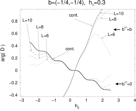
Figure 2: The argument of the normalized overlap determinant for a constant gauge background $U_{n\mu}=\mbox{e}^{2\pi ih_{\mu}/L}$ with a boundary condition $b_{\mu}=(-1/4,-1/4)$ is plotted as a function of $h_{2}$ for $h_{1}=0.3$. The boundary condition for the reference state is taken to be either $b_{\mu}^{(r)}=0$ or $b_{\mu}^{(r)}=b_{\mu}$. The continuum results (4.10) for $A_{\mu}(x)=2\pi h_{\mu}/\ell$ are shown by the bold solid lines for the corresponding $b_{\mu}^{(r)}$ .

We next examine the $b_{\mu}$ dependence of the fermion determinant for a fixed constant gauge background. In Fig. 3 we take $h_{\mu}=(0.33,0.27)$ and plot the argument of the normalized overlap determinant against $b_{2}$ for $b_{1}=-1/4$. The boundary condition for the reference state is taken to be either $b_{\mu}^{(r)}=0$ or $b_{\mu}^{(r)}=b_{\mu}$. The data for both $b_{\mu}^{(r)}$ seem to converge to the corresponding continuum results. The continuum result for $b_{\mu}^{(r)}=0$ is discontinuous at $b_{2}=\pm 1/2$. Accordingly, the convergence to the continuum limit becomes slower as $b_{2}$ gets closer to $\pm 1/2$. The continuum result for $b_{\mu}^{(r)}=b_{\mu}$, on the other hand, is a continuous function of $b_{\mu}$ and the data converge to the continuum result rapidly for all $b_{2}$.

Figure 3: The argument of the normalized overlap determinant for a constant gauge background $U_{n\mu}=\mbox{e}^{2\pi ih_{\mu}/L}$ with $h_{\mu}=(0.33,0.27)$ is plotted as a function of $b_{2}$ for $b_{1}=-1/4$. The boundary condition for the reference state is taken to be either $b_{\mu}^{(r)}=0$ or $b_{\mu}^{(r)}=b_{\mu}$. The continuum results (4.10) for $A_{\mu}(x)=2\pi h_{\mu}/\ell$ are shown by the bold solid lines for the corresponding $b_{\mu}^{(r)}$. The results for $b_{\mu}^{(r)}=b_{\mu}$ with $L\geq 10$ cannot be distinguished from the corresponding continuum result in this figure.

We next consider a more general gauge configuration. In Ref. [1], a sine-type gauge configuration has been considered for $b_{\mu}=b_{\mu}^{(r)}=0$ and the result showed a good agreement with the continuum result (2.14). In Fig. 4 we plot the argument of the normalized overlap determinant for a sine-type gauge configuration

$$U_{n\mu}=\exp\left[i\frac{\ell A^{0}_{\mu}}{L}\cos\left(\frac{2\pi k\cdot n+\pi k_{\mu}}{L}\right)\right],$$ (4.15)

with $k_{\mu}=(0,1)$ and $b_{\mu}=(-2/5,-2/5)$, against $\ell A^{0}_{2}/(2\pi)$ for a fixed $\ell A^{0}_{1}=\pi$. The boundary condition for the reference state is taken to be either $b_{\mu}^{(r)}=0$ or $b_{\mu}^{(r)}=b_{\mu}$. The data for both $b^{(r)}_{\mu}$ seem to converge to the corresponding continuum results, although finite lattice spacing effects increase for larger $|\ell A^{0}_{2}|$, as expected.

Figure 4: The argument of the normalized overlap determinant for a sine-type gauge configuration (4.15) with $k_{\mu}=(0,1)$ and $b_{\mu}=(-2/5,-2/5)$ is plotted against $\ell A^{0}_{2}/(2\pi)$ for $\ell A^{0}_{1}=\pi$. The boundary condition for the reference state is taken to be either $b_{\mu}^{(r)}=0$ or $b_{\mu}^{(r)}=b_{\mu}$. The continuum results (4.10) for the gauge configuration $A_{\mu}=A^{0}_{\mu}\cos(2\pi k\cdot x/\ell)$ are shown by the bold solid lines for the corresponding $b_{\mu}^{(r)}$.

Let us see explicitly how the overlap formalism for $b_{\mu}^{(r)}\neq b_{\mu}$ reproduces the expected translational anomaly. In Fig. 5 we plot the argument of the normalized overlap determinant for a shifted gauge configuration $U^{\prime}_{n\mu}=U_{n^{\prime}\mu}$, $n^{\prime}_{\mu}\equiv n_{\mu}-s_{\mu}$ against the shift on physical scale $(s_{1}+1/2)/L$, where the shift is taken to be symmetric in the two directions $s_{1}=s_{2}$. The original configuration is taken to be a sine-type (4.15) with $k_{\mu}=(1,0)$, $\ell A_{\mu}^{0}/(2\pi)=(0.5,0.4)$ and $b_{\mu}=(-2/5,-2/5)$. We take $b_{\mu}^{(r)}=0$. One can see that the translational anomaly given by (4.10) is clearly reproduced by the overlap formalism in the continuum limit.

Figure 5: The argument of the overlap determinant for shifted gauge configuration $U^{\prime}_{n\mu}=U_{n^{\prime}\mu}$, $n^{\prime}_{\mu}\equiv n_{\mu}-s_{\mu}$ is plotted against the shift on physical scale $(s_{1}+1/2)/L$, where the shift is taken to be symmetric in the two directions ($s_{1}=s_{2}$). We take the original configuration to be a sine-type (4.15), where $\ell A_{\mu}^{0}/(2\pi)=(0.5,0.4)$ and $k_{\mu}=(1,0)$. The boundary condition is taken to be $b_{\mu}=(-2/5,-2/5)$. For the reference state, it is taken to be antiperiodic ($b^{(r)}_{\mu}=0$). The bold solid line represents the continuum result (4.10).

Finally, we check (4.14) for a more generic case. We take the gauge configuration to be

$$U_{n\mu}=\mbox{e}^{2\pi ih_{\mu}/L}\exp\left[i\frac{\ell A_{\mu}^{0}}{L}\cos\left(\frac{2\pi k\cdot(n-s)+\pi k_{\mu}}{L}\right)\right],$$ (4.16)

where $h_{\mu}=(0.43,0.13)$, $k_{\mu}=(0,1)$ and $s_{\mu}/L=(0.2,0.6)$. The boundary conditions are taken to be $b_{\mu}=(-0.4,-0.15)$ and $b_{\mu}^{(r)}=(0.225,-0.05)$. We plot the normalized overlap determinant against $\ell A_{2}^{0}/(2\pi)$ for $\ell A_{1}^{0}/(2\pi)=0.37$. The data are seen to converge to the continuum prediction (4.10).

Figure 6: The argument of the normalized overlap determinant for a gauge configuration (4.16) with $h_{\mu}=(0.43,0.13)$, $k_{\mu}=(0,1)$ and $s_{\mu}/L=(0.2,0.6)$ is plotted against $\ell A_{2}^{0}/(2\pi)$ for $\ell A_{1}^{0}/(2\pi)=0.37$. The boundary conditions are taken to be $b_{\mu}=(-0.4,-0.15)$ and $b_{\mu}^{(r)}=(0.225,-0.05)$. The continuum result (4.10) is shown by the bold solid line.

Having confirmed that the continuum limit of the overlap formalism gives (4.14), let us discuss the physical implications of this result. We have seen that the ambiguity of the overlap formalism, which lies in the choice of the boundary condition for the reference state, corresponds to the phase ambiguity of the chiral determinant on a two-dimensional torus proportional to the Polyakov loops along the boundaries. This gives rise to a translational anomaly in general. The identity (4.4) shows that translational invariance can be preserved by taking $b_{\mu}^{(r)}=b_{\mu}$. On the other hand, the identity (4.6) shows that, when one absorbs a delta-function like singularity in the gauge field by a change of the boundary condition for the fermion, $b_{\mu}^{(r)}$ should be kept fixed. Therefore, the requirement on the fermion determinant that a delta-function like singularity in the gauge field can be absorbed by a change of the boundary condition for the fermion, is not compatible with translational invariance. Note that this feature is not restricted to the 2D U(1) case, since (4.4) and (4.6) hold for general chiral gauge theories on a torus.

5 Symmetries of the fermion determinant

In this section, we examine the ambiguity of $b_{\mu}^{(r)}$ from the viewpoint of symmetries that the fermion determinant should possess for a general chiral gauge theory. We consider the space-time symmetries, such as chirality interchange, parity transformation, charge conjugation and a 90^∘ rotation, which have been discussed in Ref. [1] in the infinite volume. What we do here is to repeat their argument for a finite lattice with arbitrary boundary conditions for fermions.

Here we need to consider Weyl fermions with the opposite chirality. In the overlap formalism, the fermion determinant for a left-handed Weyl fermion, namely with the opposite chirality to the one we have been considering, can be obtained [1] by simply flipping the sign of the many-body Hamiltonians (3.1) and (3.7) for the right-handed Weyl fermion. We denote the fermion determinant for each chirality defined within the overlap formalism by $D_{lat}^{R}$ and $D_{lat}^{L}$, respectively. Note that $D_{lat}^{R}(U_{n\mu},b_{\mu};b_{\mu}^{(r)})$ and $D_{lat}^{L}(U_{n\mu},b_{\mu};b_{\mu}^{(r)})$ have a phase ambiguity independent of both $U_{n\mu}$ and $b_{\mu}$ for each $b_{\mu}^{(r)}$. Here we assume that this residual phase ambiguity has been fixed by requiring that the fermion determinant be real positive for $U_{n\mu}=1$ and $b_{\mu}=b_{\mu}^{(r)}$. Then the following statements hold for any chiral gauge theory in any even dimension $D$.

(i) chirality interchange

The relation between $D_{lat}^{R}$ and $D_{lat}^{L}$ is given as

$$D_{lat}^{R}(U_{n\mu},b_{\mu};b^{(r)}_{\mu})=D_{lat}^{L}(U_{n\mu},b_{\mu};b^{(r)}_{\mu})^{*}.$$ (5.1)

(ii) parity transformation

We consider the parity transformation of the gauge field:

$$U^{P}_{n\mu}=\left\{\begin{array}[]{ll}U_{n^{P},-\mu}&\mbox{for}~{}~{}~{}\mu=1,...,D-1\\ U_{n^{P},\mu}&\mbox{for}~{}~{}~{}\mu=D,\end{array}\right.$$ (5.4)

where $n^{P}_{\mu}$ is defined by

$$n^{P}_{\mu}=\left\{\begin{array}[]{ll}(L-1)-n_{\mu}&\mbox{for}~{}~{}~{}\mu=1,...,D-1\\ n_{\mu}&\mbox{for}~{}~{}~{}\mu=D.\end{array}\right.$$ (5.5)

$U_{n,-\mu}$ is defined as usual by the hermitian conjugate of the link variable residing on a link which stems from the site $n_{\mu}$ to the $-\mu$ direction and can be given explicitly as

$$U_{n,-\mu}=\left\{\begin{array}[]{ll}U_{n-\hat{\mu},\mu}^{\dagger}&\mbox{for}~{}~{}~{}~{}~{}n_{\mu}=1,...,L-1\\ U_{n+(L-1)\hat{\mu},\mu}^{\dagger}&\mbox{for}~{}~{}~{}~{}~{}n_{\mu}=0.\end{array}\right.$$ (5.6)

Then, we have

$$D_{lat}^{R}(U_{n\mu},b_{\mu};b^{(r)}_{\mu})=D_{lat}^{L}(U^{P}_{n\mu},b^{P}_{\mu};b^{(r)P}_{\mu}),$$ (5.7)

where $b^{P}_{\mu}$ is given by

$$b_{\mu}^{P}=\left\{\begin{array}[]{ll}-b_{\mu}&\mbox{for}~{}~{}~{}\mu=1,...,D-1\\ b_{\mu}&\mbox{for}~{}~{}~{}\mu=D,\\ \end{array}\right.$$ (5.8)

and $b_{\mu}^{(r)P}$ is defined similarly.

(iii) charge conjugation

Under the charge conjugation of the gauge field, we have

$$D_{lat}^{R}(U_{n\mu},b_{\mu};b^{(r)}_{\mu}) = D_{lat}^{R}(U^{*}_{n\mu},-b_{\mu};-b^{(r)}_{\mu})~{}~{}\mbox{for}~{}~{}~{}D=2,$$ (5.9)

$$D_{lat}^{R}(U_{n\mu},b_{\mu};b^{(r)}_{\mu}) = D_{lat}^{L}(U^{*}_{n\mu},-b_{\mu};-b^{(r)}_{\mu})~{}~{}\mbox{for}~{}~{}~{}D=4,$$ (5.10)

and similar relations for $D\geq 6$.

(iv) 90^∘ rotational invariance

We consider a 90^∘ rotation in the ($\alpha$,$\beta$) plane, where $1\leq\alpha<\beta\leq D$. The gauge configuration is transformed as

$$U^{rot}_{n\mu}=\left\{\begin{array}[]{ll}U_{n^{rot},\beta}&\mbox{for}~{}~{}~{}\mu=\alpha\\ U_{n^{rot},-\alpha}&\mbox{for}~{}~{}~{}\mu=\beta\\ U_{n^{rot},\mu}&\mbox{otherwise},\end{array}\right.$$ (5.14)

where $n^{rot}_{\mu}$ is defined by

$$n^{rot}_{\mu}=\left\{\begin{array}[]{ll}n_{\beta}&\mbox{for}~{}~{}~{}\mu=\alpha\\ (L-1)-n_{\alpha}&\mbox{for}~{}~{}~{}\mu=\beta\\ n_{\mu}&\mbox{otherwise},\end{array}\right.$$ (5.15)

and $U_{n,-\mu}$ is defined by (5.6). Then, we have

$$D_{lat}^{R}(U_{n\mu},b_{\mu};b^{(r)}_{\mu})=D_{lat}^{R}(U^{rot}_{n\mu},b^{rot}_{\mu};b^{(r)rot}_{\mu}),$$ (5.16)

where $b^{rot}_{\mu}$ is given by

$$b_{\mu}^{rot}=\left\{\begin{array}[]{ll}b_{\beta}&\mbox{for}~{}~{}~{}\mu=\alpha\\ -b_{\alpha}&\mbox{for}~{}~{}~{}\mu=\beta\\ b_{\mu}&\mbox{otherwise},\\ \end{array}\right.$$ (5.17)

and $b_{\mu}^{(r)rot}$ is defined similarly.

These behaviors are the ones we expect in the continuum if we consider $b_{\mu}^{(r)}$ as a parameter representing an external source. If we regard $b_{\mu}^{(r)}$ as a regularization parameter, which should be fixed as a function of $b_{\mu}$, the allowed choices for $b_{\mu}^{(r)}$ are (A) $b_{\mu}^{(r)}=b_{\mu}$, (B) $b_{\mu}^{(r)}\equiv 0$, and (C) $b_{\mu}^{(r)}\equiv\pi$. For the 2D U(1) case, (A) and (B) correspond to the results given by eqs. (2.22) and (2.19), respectively. (C) has not been encountered in Section 2, since we started from the known result for $b_{\mu}=0$, for which the phase choice corresponding to (C) becomes ill-defined. As we have seen in Section 4, (A) can be singled out by imposing the translational invariance, but only by sacrificing the property that a singularity in the gauge configuration can be absorbed by a change of the boundary condition for the fermion.

6 Singular gauge background

In Ref. [7], it was discovered that 2D U(1) chiral gauge theories have an anomaly under singular gauge transformations in general, even if the gauge anomaly for non-singular gauge transformations is cancelled. We first point out that there is actually an ambiguity in the calculation of chiral determinants in the continuum when the gauge configuration has a delta-function like singularity. A typical configuration we consider here is given by

$$A^{s}_{\mu}(x)=A_{\mu}(x)+2\pi c_{\mu}\delta(x_{\mu}-\tilde{x}_{\mu}),$$ (6.1)

where $A_{\mu}(x)$ is a non-singular function and $c_{\mu}$ is a real coefficient.

Let us consider first regularizing the delta-function like singularity as

$$A^{reg}_{\mu}(x)=A_{\mu}(x)+2\pi c_{\mu}f(x_{\mu}-\tilde{x}_{\mu}),$$ (6.2)

where $f(t)$ is a non-singular function which we send to $\delta(t)$ in the end. We use (4.10) for the non-singular gauge configuration $A^{reg}_{\mu}(x)$ and finally take the limit $f(t)\rightarrow\delta(t)$. The result we obtain in this way is

$$D_{\mbox{\scriptsize I}}(A^{s}_{\mu},b_{\mu};b_{\mu}^{(r)}) = \mbox{e}^{i\xi}D\left(A_{\mu}+\frac{2\pi c_{\mu}}{\ell},b_{\mu};b_{\mu}^{(r)}\right),$$ (6.3)

$$\xi = -\frac{1}{2}\left[c_{1}\left.\int\mbox{d}x_{2}\partial_{1}\phi\right|_{x_{1}=\tilde{x}_{1}}+c_{2}\left.\int\mbox{d}x_{1}\partial_{2}\phi\right|_{x_{2}=\tilde{x}_{2}}\right].$$ (6.4)

Note that the result is not invariant under $c_{\mu}\rightarrow c_{\mu}+n_{\mu}$.

On the other hand, we can treat the singularity in the gauge configuration just as we did in Section 2 when we considered a change of the boundary condition for the fermion as a singularity in the gauge configuration.

When the singularity resides exactly on the boundary, namely for $\tilde{x}_{\mu}=0$, the singularity should not be distinguished from the boundary condition, and therefore we have

$$D_{\mbox{\scriptsize II(a)}}(A^{s}_{\mu},b_{\mu};b_{\mu}^{(r)})=D(A_{\mu},b_{\mu}+c_{\mu};b_{\mu}^{(r)}).$$ (6.5)

This is the case considered in Ref. [7]. For $\tilde{x}_{\mu}\neq 0$, one can follow the same steps as we did in deriving (2.19) and arrive at

$$D_{\mbox{\scriptsize II(b)}}(A^{s}_{\mu},b_{\mu};b_{\mu}^{(r)}) = \mbox{e}^{i\zeta}D\left(A_{\mu}+\frac{2\pi P[c_{\mu}]}{\ell},b_{\mu};b_{\mu}^{(r)}\right),$$ (6.6)

$$\zeta = -\frac{1}{2}\left[P[c_{1}]\left.\int\mbox{d}x_{2}\partial_{1}\phi\right|_{x_{1}=\tilde{x}_{1}}+P[c_{2}]\left.\int\mbox{d}x_{1}\partial_{2}\phi\right|_{x_{2}=\tilde{x}_{2}}\right].$$ (6.7)

The only difference between (6.6) and (6.3) is that we now have the projection function $P$ acting on $c_{\mu}$. They coincides for $|c_{\mu}|<1/2$, but not in general. Using the identity (4.13), one finds that the difference can occur only in the phase. Both (6.5) and (6.6) are invariant under $c_{\mu}\rightarrow c_{\mu}+n_{\mu}$ as they should. (6.6) in the limit of $\tilde{x}_{\mu}\rightarrow 0$ is not necessarily equal to (6.5). One can show that they are equal for the following two cases :

(i) $b_{\mu}^{(r)}=b_{\mu}$

(ii) $b_{\mu}^{(r)}=0$ and $|P[b_{\mu}]+P[c_{\mu}]|<\frac{1}{2}$,

but not in general. (i) is expected since the translational invariance is manifestly preserved for this choice of $b_{\mu}^{(r)}$. One finds that the discontinuity can occur only in the phase, again, using the identity (4.13). On the other hand, $D_{\mbox{\scriptsize I}}$ given by (6.3) has no discontinuity at $\tilde{x}_{\mu}=0$ at all.

Thus the continuum result for $D(A_{\mu}^{s},b_{\mu};b_{\mu}^{(r)})$ can be given by $D_{\mbox{\scriptsize I}}$ or $D_{\mbox{\scriptsize II}}$ depending on how one treats the singular gauge configuration (6.1). $D_{\mbox{\scriptsize I}}$ is the one given by a limit of (4.10), but $D_{\mbox{\scriptsize II}}$ cannot be obtained this way. We should also note that the ambiguity for singular gauge configurations is exactly due to the lack of gauge invariance for a single Weyl fermion. As a consequence, the ambiguity lies only in the phase factor. In vector-like gauge theories, the singularity, no matter how one puts it on the lattice, can always be spread out over the whole space-time by a gauge transformation as we will see in the next section. Thus the ambiguity for singular gauge configurations as well as the translational anomaly is peculiar to chiral gauge theories. In what follows, we will see that this ambiguity can be reproduced by the overlap formalism.

Within the overlap formalism, the ambiguity arises when one puts the continuum singular configurations such as (6.1) on the lattice. $D_{\mbox{\scriptsize I}}$ can be reproduced by putting $A_{\mu}^{reg}$ on the lattice as in (4.2). After taking the continuum limit, one takes $f(t)$ to $\delta(t)$. (6.3) can be trivially reproduced once one admits that (4.14) holds for $U_{n\mu}$ related to a non-singular $A_{\mu}(x)$ through (4.2).

$D_{\mbox{\scriptsize II}}$ can be reproduced by putting the singular gauge configuration (6.1) on the lattice as

$$U^{s}_{n\mu}=\left\{\begin{array}[]{ll}\mbox{e}^{2\pi ic_{\mu}}U_{n\mu}&\mbox{for}~{}~{}~{}n_{\mu}=\tilde{n}_{\mu}\\ U_{n\mu}&\mbox{otherwise},\end{array}\right.$$ (6.8)

where $U_{n\mu}$ is related to $A_{\mu}(x)$ in (6.1) through (4.2) and $\tilde{x}_{\mu}=\tilde{n}_{\mu}a$.

Figure 7: The same plot as in Fig. 5 except that we take the original configuration to be a singular gauge configuration, $U_{n\mu}^{s}$ given by (6.8) with $U_{n\mu}=1$, $\tilde{n}_{\mu}=L-1$ and $c_{\mu}=(0.2,0.4)$. The boundary condition is taken to be $b_{\mu}=(-1/4,1/4)$. The boundary condition for the reference state is taken to be antiperiodic ($b^{(r)}_{\mu}=0$). We take the shift to be symmetric in the two directions ($s_{1}=s_{2}$), and plot the result against the shift $s_{1}/L$ on physical scale. The arrow with “sing(a)” represents the continuum prediction (6.5) for the case in which the singularity resides exactly on the boundary. The horizontal line denoted as “sing(b)” represents the continuum prediction (6.6) for the case in which the singularity resides off the boundary.

There are actually many other ways to put the singular gauge configuration on the lattice, between these two extremes, since one can spread the singularity on two links or as many links as one likes. If one naively applies the formula (4.2), one obtains (6.8). Note, however, that all the other lattice configurations go to (6.1) in the continuum limit and therefore can be considered as equally good lattice regularizations of (6.1). The important point is that the result depends on which way we adopt for discretizing the singularity (6.1). We also recall that in Section 2 we considered a change of the boundary condition for the fermion as a singularity in the gauge configuration. There we didn’t have this ambiguity and we put the singularity on a single link, since boundary conditions should be imposed literally on the boundary. But this is not the case when we discuss singularities in gauge configurations.

Let us check that $D_{\mbox{\scriptsize II}}$ given by (6.5) for $\tilde{x}_{\mu}=0$ and by (6.6) for $\tilde{x}_{\mu}\neq 0$ can be reproduced by the overlap formalism. In Fig. 7 we make a plot similar to the one we made in Fig. 5 except that we consider a singular gauge configuration. We take the original configuration to be (6.8) with $U_{n\mu}=1$, $\tilde{n}_{\mu}=L-1$ and $c_{\mu}=(0.2,0.4)$. We take $b_{\mu}=(-1/4,1/4)$ and $b_{\mu}^{(r)}=0$. We find that the result expected in the continuum is reproduced clearly. Note again that for $b_{\mu}^{(r)}=0$ the gap at $s_{1}/L=0$ disappears when $|P[b_{\mu}]+P[c_{\mu}]|<1/2$. If we took the boundary condition to be $b_{\mu}=(1/4,-1/4)$ with the same $c_{\mu}$, the gap would disappear in the continuum limit. We have also checked this numerically.

7 Constructing anomaly free gauge theories

In this section, we reconsider the gauge anomaly under singular gauge transformations discovered in Ref. [7].

There are two kinds of gauge transformation in the present model. One is

$$A_{\mu}\rightarrow A_{\mu}+\partial_{\mu}\Lambda,$$ (7.1)

which is a gauge transformation that can be obtained by repeated use of infinitesimal gauge transformations. Let us call it a “small” gauge transformation. The other one is

$$A_{\mu}\rightarrow A_{\mu}+\frac{2\pi n_{\mu}}{\ell},$$ (7.2)

where $n_{\mu}$ is an integer vector. This is what we call a “large” gauge transformation, which has a nontrivial topology and cannot be obtained by repeated use of infinitesimal gauge transformations. If we decompose the gauge background $A_{\mu}$ as in (2.9), (7.1) gives $\chi\rightarrow\chi+\Lambda$, whereas (7.2) gives $h_{\mu}\rightarrow h_{\mu}+n_{\mu}$, where $h_{\mu}=\frac{\ell\alpha_{\mu}}{2\pi}$ as before.

Let us first restrict ourselves to non-singular gauge configurations. Then we only have to consider (4.10). The exact result (4.10) for a single Weyl fermion is not invariant under the above two kinds of gauge transformation, which is nothing but the gauge anomaly. In order to cancel the gauge anomaly, we have to add extra Weyl fermions. Note that the fermion determinant for a right-handed fermion is given by (4.10), and by its complex conjugate for a left-handed fermion, both with a unit charge. For charge $q$ fermion, $h_{\mu}$, $\phi$ and $\chi$ should be multiplied by $q$ in the corresponding formulae for fermions with a unit charge. Let us consider a model with $N_{R}$ right-handed fermion with charge $q^{R}_{i}$ ($i=1,\cdots,N_{R}$) with boundary conditions parametrized by $b^{R}_{\mu i}$, and $N_{L}$ left-handed fermion with charge $q^{L}_{i}$ ($i=1,\cdots,N_{L}$) with boundary conditions parametrized by $b^{L}_{\mu i}$. Let us denote the fermion determinant of the whole system as $D(A_{\mu}(x),b^{R}_{\mu i},b^{L}_{\mu i};b^{R(r)}_{\mu i},b^{L(r)}_{\mu i})$, which is nothing but the product of the corresponding fermion determinant for each fermion. By referring to the exact results, one can easily find the condition for the invariance of $D(A_{\mu}(x),b^{R}_{\mu i},b^{L}_{\mu i};b^{R(r)}_{\mu i},b^{L(r)}_{\mu i})$ under (7.1) and (7.2). The invariance under a small gauge transformation (7.1) requires

$$\sum_{i=1}^{N_{R}}(q^{R}_{i})^{2}=\sum_{i=1}^{N_{L}}(q^{L}_{i})^{2}.$$ (7.3)

The invariance under a large gauge transformation (7.2) further requires

$$\sum_{i=1}^{N_{R}}q^{R}_{i}\left(P[b^{R}_{i\mu}]-\frac{1}{2}P[b^{R}_{i\mu}-b^{R(r)}_{i\mu}]\right)-\sum_{i=1}^{N_{L}}q^{L}_{i}\left(P[b^{L}_{i\mu}]-\frac{1}{2}P[b^{L}_{i\mu}-b^{L(r)}_{i\mu}]\right)=m_{\mu},$$ (7.4)

where $m_{\mu}$ is an integer vector. We have used the identity (4.13).

The condition for translational invariance is given by

$$\sum_{i=1}^{N_{R}}q^{R}_{i}P[b^{R}_{i\mu}-b^{R(r)}_{i\mu}]-\sum_{i=1}^{N_{L}}q^{L}_{i}P[b^{L}_{i\mu}-b^{L(r)}_{i\mu}]=0.$$ (7.5)

This means that the translational invariance can have an anomaly even if both (7.3) and (7.4) are satisfied.

Now let us also consider singular gauge configurations $A^{s}_{\mu}$ given by (6.1). In this case, it is not sufficient to consider only (4.10) as we explained in the previous section. Therefore, the gauge invariance might be violated even if (7.3) and (7.4) are satisfied. Likewise, the translational invariance might be violated even if (7.5) is satisfied. Indeed, this is what happens.

As stated in Ref. [7], $A^{s}_{\mu}$ can be gauge-transformed to a configuration $A^{u}_{\mu}$, which does not have a delta-function like singularity as

$$A^{s}_{\mu}(x) = A^{u}_{\mu}(x)+\partial_{\mu}\Lambda(x;\tilde{x},c),$$ (7.6)

$$A^{u}_{\mu}(x) \stackrel{{\scriptstyle\rm def}}{{=}} A_{\mu}(x)+\frac{2\pi c_{\mu}}{\ell}.$$ (7.7)

The transformation function $\Lambda(x;\tilde{x},c)$ is given by

$$\Lambda(x;\tilde{x},c)=-\frac{2\pi c_{1}}{\ell}\Xi(x_{1};\tilde{x}_{1})-\frac{2\pi c_{2}}{\ell}\Xi(x_{2};\tilde{x}_{2}),$$ (7.8)

where

$$\Xi(t;\tilde{t})=\left\{\begin{array}[]{ll}t&\mbox{for}~{}~{}~{}0<t<\tilde{t}\\ t-\ell&\mbox{for}~{}~{}~{}\tilde{t}<t<\ell.\end{array}\right.$$ (7.9)

This gauge transformation is singular in the sense that $\Lambda(x;\tilde{x},c)$ has a discontinuity on $\{x_{1}=\tilde{x}_{1}\}\cup\{x_{2}=\tilde{x}_{2}\}$ as a function on the 2-dimensional torus. Note also that changing the location of the singularity $\tilde{x}_{\mu}$ can be achieved by successive singular gauge transformations.

In order to construct an anomaly-free chiral gauge theory, the fermion determinant should be invariant under such singular gauge transformations as well, namely,

$$D(A^{s}_{\mu}(x),b^{R}_{\mu i},b^{L}_{\mu i};b^{R(r)}_{\mu i},b^{L(r)}_{\mu i})=D(A^{u}_{\mu}(x),b^{R}_{\mu i},b^{L}_{\mu i};b^{R(r)}_{\mu i},b^{L(r)}_{\mu i}).$$ (7.10)

Obviously, the consequence of this requirement depends on which of $D_{\mbox{\scriptsize I}}$ and $D_{\mbox{\scriptsize II}}$ we consider as the continuum result for the singular gauge configuration $A_{\mu}^{s}$. If we consider $D_{\mbox{\scriptsize I}}$, (7.10) is satisfied automatically, so long as (7.3) is satisfied, since $D_{\mbox{\scriptsize I}}$ can be obtained as a limit of (4.10).

If we consider $D_{\mbox{\scriptsize II}}$, on the other hand, the absence of the gauge anomaly under singular gauge transformations does not automatically follow from (7.3) and (7.4) and puts an additional condition which should be satisfied by the theory in order to make it anomaly free. The phase choice of the fermion determinant adopted in Ref. [7] corresponds to taking an antiperiodic boundary condition for all the fermion species irrespective of the boundary conditions for these fermions; namely $b^{R(r)}_{\mu i}=b^{L(r)}_{\mu i}=0$. The argument was restricted to the case when the singularity in the gauge configuration resides exactly on the boundary. Referring to (6.5), we find that the condition is

$$D\left(A_{\mu}(x)+\frac{2\pi c_{\mu}}{\ell},b^{R}_{\mu i},b^{L}_{\mu i};b^{R(r)}_{\mu i}=0,b^{L(r)}_{\mu i}=0\right)$$ (7.11)

$$= D(A_{\mu}(x),b^{R}_{\mu i}+q^{R}_{i}c_{\mu},b^{L}_{\mu i}+q^{L}_{i}c_{\mu};b^{R(r)}_{\mu i}=0,b^{L(r)}_{\mu i}=0).$$

As claimed in Ref. [7], this is not always satisfied even if (7.3) and (7.4) hold. For example, a model with four right-handed fermions with a unit charge and one left-handed fermion with charge two, all of which obeying an antiperiodic boundary condition, satisfies (7.3) and (7.4), but not (7.11). This led the authors of Ref. [7] to twist the boundary conditions as

$$b^{R}_{1\mu}=\left(\frac{1}{4},\frac{1}{4}\right);~{}~{}~{}b^{R}_{2\mu}=\left(\frac{1}{4},-\frac{1}{4}\right);~{}~{}~{}b^{R}_{3\mu}=\left(-\frac{1}{4},\frac{1}{4}\right);~{}~{}~{}b^{R}_{4\mu}=\left(-\frac{1}{4},-\frac{1}{4}\right);~{}~{}~{}b^{L}_{1\mu}=(0,0),$$ (7.12)

with which one can satisfy (7.11) as well. Let us call the former model “antiperiodic 11112 model” and the latter “twisted 11112 model”.

Figure 8: The argument of the normalized overlap determinant for the twisted 11112 model. As singular gauge configurations we take, $U_{n\mu}^{s}$ given by (6.8) with $U_{n\mu}=1$, $c_{1}=0.185$. “sing(a)” represents the results for $\tilde{n}_{\mu}=L-1$, where as “sing(b)” represents the results for $\tilde{n}_{\mu}=L/2-1$. “uniform” represents the results for the uniform gauge configurations $U_{n\mu}^{u}=\mbox{e}^{2\pi ic_{\mu}/L}$, which can be obtained by a gauge transformation from $U_{n\mu}^{s}$. The horizontal axis represents $c_{2}$.

Since the translational invariance is not preserved with that phase choice of the fermion determinant, however, one should also consider the case when the singularity does not coincide with the boundary. Referring to (6.6), one finds that (7.10) is satisfied if $|q_{i}^{L}c_{\mu}|<1/2$ and $|q_{i}^{R}c_{\mu}|<1/2$ for all $i$, but not in general, even if (7.3), (7.4) and (7.11) are satisfied. This is illustrated in Fig. 8 for the twisted 11112 model. As singular gauge configurations, we consider $U_{n\mu}^{s}$ given by (6.8) with $U_{n\mu}=1$, $c_{1}=0.185$. “sing(a)” represents the results for $\tilde{n}_{\mu}=L-1$, whereas “sing(b)” represents the results for $\tilde{n}_{\mu}=L/2-1$. “uniform” represents the results for the uniform gauge configurations $U_{n\mu}^{u}=\mbox{e}^{2\pi ic_{\mu}/L}$, which can be obtained by a gauge transformation from $U_{n\mu}^{s}$. We plot the argument of the normalized overlap determinant for the twisted 11112 model as a function of $c_{2}$. We only show the results for positive $c_{2}$. Note that the fermion determinants for $-c_{2}$ for the three types of configurations we consider in Fig. 8 can be obtained by taking the complex conjugate of those for $c_{2}$. This can be shown by using the parity transformation property (5.7). The normalized fermion determinants for the uniform gauge configurations are real positive in the continuum as noted in Ref. [7]. This is seen to be reproduced by the overlap formalism in Fig. 8. When the singularity coincides with the boundary (sing(a) in Fig. 8), the results agree with those for the uniform gauge configurations. A slight discrepancy seen near $c_{2}=1/4$ can be understood if we look at the fermion determinant for each species separately. One finds that the results for the charge-2 left-handed fermion and those for the charge-1 right-handed fermions with $b^{R}_{i2}=1/4$ have gaps at $c_{2}=1/4$ and the gaps are expected to cancel each other in the continuum limit. Therefore, the discrepancy is considered to be a finite lattice spacing effect. On the other hand, when the singularity is off the boundary (sing(b) in Fig. 8), the results agree with those for the uniform gauge configurations for $c_{2}<1/4$, but not for $c_{2}>1/4$ as expected. The gap seen at $c_{2}=1/4$ is due to the charge-2 left-handed fermion, and the one seen at $c_{2}=1/2$ is due to the charge-1 right-handed fermions. The approach to the continuum prediction is slow near these gaps.

Figure 9: The same plot as in Fig. 8, except that we take the boundary condition for the reference state to be $b_{\mu}^{(r)}=b_{\mu}$. Since the translational invariance is manifestly preserved on the lattice for this choice of $b_{\mu}^{(r)}$, the results for the singular gauge configurations, which are denoted as “sing”, do not depend on $\tilde{n}_{\mu}$, the location of the singularity.

The above argument shows that if we consider $D_{\mbox{\scriptsize II}}$ as the continuum result for the singular gauge configurations, even the twisted 11112 model is not completely anomaly-free. Note also that for the boundary condition (7.12), (7.5) is satisfied. However, the translational invariance is broken as is seen above, because we are considering singular gauge configurations, which are not considered in deriving (7.5).

When we consider the case in which the singularity of the gauge configuration is off the boundary, the choice of the boundary conditions makes no difference to the anomaly for singular gauge transformations. Actually there is no way to cancel the anomaly under singular gauge transformations except by putting a copy of fermions with the same charge and the same boundary condition but with the opposite chirality, which makes the theory vector-like. This conclusion does not depend on the choice of $b_{\mu}^{(r)}$. In particular, the conclusion remains unchanged even if we take the translationally invariant choice $b_{\mu}^{(r)}=b_{\mu}$. This is illustrated in Fig. 9. Due to the translational invariance, the results for the singular gauge configurations do not depend on the location of the singularity. They agree with the results for the uniform gauge configurations for $c_{2}<1/4$, but not for $c_{2}>1/4$.

8 Generalization to other dimensions

In this section, we generalize our main results to any even dimension for the abelian case. We discuss the translation anomaly, the ambiguity in the continuum calculation of chiral determinants for singular gauge configurations, and the gauge anomaly under singular gauge transformations. Although we do not know the exact results for chiral determinants except in two dimensions, we can address the above issues only by using the knowledge of gauge anomaly.

We denote the translationally invariant chiral determinant for a single right-handed Weyl fermion on a torus of general even dimension as $D(A_{\mu},b_{\mu})$. We define the current $j_{\mu}[A]$ by

$$j_{\mu}[A]=\frac{\delta}{\delta A_{\mu}(x)}\ln D(A_{\nu},b_{\nu}).$$ (8.1)

The anomaly equation is given by

$$\partial_{\mu}j_{\mu}=i\partial_{\mu}K_{\mu}[A],$$ (8.2)

where $K_{\mu}[A]$ is defined for $D=2p$ by

$$K_{\mu}[A]=\frac{1}{2(2\pi)^{p}p!}\epsilon_{\mu\nu_{1}\mu_{2}\nu_{2}\cdots\mu_{p}\nu_{p}}A_{\nu_{1}}\partial_{\mu_{2}}A_{\nu_{2}}\cdots\partial_{\mu_{p}}A_{\nu_{p}}.$$ (8.3)

Let us consider a singular gauge configuration $A_{\mu}^{s}(x)$ given by (6.1), where $\tilde{x}_{\mu}$ and $c_{\mu}$ represent the location and the strength of the singularity, respectively. As we discussed in Section 6, the continuum calculation of $D(A_{\mu}^{s}(x),b_{\mu})$ has an ambiguity corresponding to (6.3) and (6.6) in $D=2$. We denote the two possible results as $D_{\mbox{\scriptsize I}}(A_{\mu}^{s}(x),b_{\mu})$ and $D_{\mbox{\scriptsize II}}(A_{\mu}^{s}(x),b_{\mu})$ in the present case. Let us first consider $D_{\mbox{\scriptsize I}}(A_{\mu}^{s}(x),b_{\mu})$. We recall that $A^{s}_{\mu}$ can be gauge-transformed to a configuration $A^{u}_{\mu}$ given by (7.7), which does not have any singularity, by a gauge transformation (7.6) with the transformation function $\Lambda(x;\tilde{x},c)$ given by (7.8). We, therefore, obtain

$$\ln D_{\mbox{\scriptsize I}}(A_{\mu}^{s}(x),b_{\mu})-\ln D(A_{\mu}^{u}(x),b_{\mu})=-i\int\mbox{d}^{D}x~{}\Lambda(x;\tilde{x},c)\partial_{\mu}K_{\mu}[A],$$ (8.4)

where we have used the fact that $\partial_{\mu}K_{\mu}$ is invariant under a gauge transformation $A_{\mu}\rightarrow A_{\mu}+\partial_{\mu}\Lambda$ and a constant shift $A_{\mu}\rightarrow A_{\mu}+\alpha_{\mu}$. Differentiating both sides of (8.4) with respect to $\tilde{x}_{\mu}$, we obtain

$$\frac{\partial}{\partial\tilde{x}_{\mu}}\ln D_{\mbox{\scriptsize I}}(A_{\mu}^{s}(x),b_{\mu})=2\pi ic_{\mu}\left.\frac{\partial}{\partial\tilde{x}_{\mu}}\int\mbox{d}^{D-1}x~{}K_{\mu}[A]\right|_{x_{\mu}=\tilde{x}_{\mu}}.$$ (8.5)

The integral on the r.h.s. of (8.5) yields the Chern-Simons action on the boundaries in general. The corresponding result for $D_{\mbox{\scriptsize II}}$ can be obtained by simply replacing $c_{\mu}$ by $P[c_{\mu}]$ in (8.5).

$$\frac{\partial}{\partial\tilde{x}_{\mu}}\ln D_{\mbox{\scriptsize II}}(A_{\mu}^{s}(x),b_{\mu})=2\pi iP[c_{\mu}]\left.\frac{\partial}{\partial\tilde{x}_{\mu}}\int\mbox{d}^{D-1}x~{}K_{\mu}[A]\right|_{x_{\mu}=\tilde{x}_{\mu}}.$$ (8.6)

One can see that these results are consistent with (6.3) and (6.6) in $D=2$ by using (8.3). (8.5) and (8.6) are equal for $|c_{\mu}|<1/2$, but not in general.

Let us then discuss the translational anomaly. We define $D(A_{\mu},b_{\mu};b_{\mu}^{(r)})$ as in (4.8) and (4.9) in any even dimension. We note that

$$D(A_{\mu}(x+\tilde{x}),b_{\mu};b_{\mu}^{(r)})=D_{\mbox{\scriptsize II}}(A_{\mu}^{s}(x),b_{\mu}),$$ (8.7)

where $c_{\mu}$ in $A_{\mu}^{s}(x)$ should be taken to be $c_{\mu}=b_{\mu}-b_{\mu}^{(r)}$. Therefore, non-vanishing of (8.6) immediately implies the existence of translational anomaly. The translational anomaly vanishes for $b_{\mu}^{(r)}=b_{\mu}$ as it should. From this result, we can deduce that the effect of having $b_{\mu}^{(r)}$ different from $b_{\mu}$ is essentially given by the phase factor proportional to the Chern-Simons action on the boundaries up to an irrelevant constant factor; namely,

$$D(A_{\mu}(x),b_{\mu};b_{\mu}^{(r)}) \sim \mbox{e}^{i\beta}D(A_{\mu},b_{\mu}),$$ (8.8)

$$\beta = 2\pi\left.\sum_{\mu=1}^{D}P[b_{\mu}-b_{\mu}^{(r)}]\int\mbox{d}^{D-1}x~{}K_{\mu}[A]\right|_{x_{\mu}=0}.$$ (8.9)

Note that the extra phase factor does not affect the anomaly equation (8.2), since the Chern-Simons action is invariant under small gauge transformations. (8.8) is consistent with (4.10) in $D=2$.

Let us finally discuss the gauge anomaly under singular gauge transformations. Here we consider the translationally invariant case $b_{\mu}^{(r)}=b_{\mu}$. The conclusion is the same for $b_{\mu}^{(r)}\neq b_{\mu}$ as long as the singularity is off the boundary. We consider the singular gauge configuration $A_{\mu}^{s}(x)$. We recall that changing the location of the singularity is a gauge transformation, which can be achieved by successive singular gauge transformations. Eqs. (8.5) and (8.6), therefore, give the gauge anomaly for a single right-handed Weyl fermion under this gauge transformation. Let us then consider an anomaly-free fermion content which satisfies a charge relation corresponding to (7.3) in 2D and see whether the above gauge anomaly is cancelled as well. When we consider $D_{\mbox{\scriptsize I}}$, the gauge anomaly (8.5) automatically cancels due to the charge relation. When we consider $D_{\mbox{\scriptsize II}}$, however, the gauge anomaly (8.6) cancels when $|q_{i}^{L}c_{\mu}|<1/2$ and $|q_{i}^{R}c_{\mu}|<1/2$, but not in general.

Thus we have seen that U(1) chiral gauge theories on a torus in any even dimension have the translational anomaly and the singular gauge anomaly, and that the latter suffers from an ambiguity in the continuum calculation of chiral determinants for singular gauge configurations.

9 Summary and Discussions

In this paper, we pointed out that the fermion determinant in chiral gauge theories on a two-dimensional torus can have a phase ambiguity, which is proportional to the Polyakov loops along the boundaries. The continuum results have been reproduced by the overlap formalism, where the phase ambiguity comes from the ambiguity of the formalism, which lies in the boundary condition for the reference state used in the Wigner-Brillouin phase choice. The anomaly equation is not affected by the ambiguous phase factor and therefore cannot fix the ambiguity. Space-time symmetries, such as chirality interchange, parity transformation, charge conjugation and 90^∘ rotation almost fix the ambiguity, but not completely. One can fix it completely by imposing the translational invariance, which corresponds, in the overlap formalism, to taking the boundary condition for the reference state to be identical to the one for the fermion under consideration. But then the fermion determinant loses the property that a singularity in the gauge configuration can be absorbed by a change of the boundary condition for the fermion. The conflict between the translational invariance and the absorption of the gauge field singularity by a change of the boundary condition, is realized by the overlap formalism on the lattice for general chiral gauge theories on a torus.

Using these new insights, we reconsidered the gauge anomaly under singular gauge transformations discovered in Ref. [7]. We pointed out that the phase choice adopted there actually corresponds to the one which breaks translational invariance and that the argument was restricted to the case in which the singularity in the gauge field resides exactly on the boundary. If one shifts the singularity off the boundary, the result changes because of the lack of translational invariance. Taking this case into account, there is no way to make completely anomaly-free 2D U(1) chiral gauge theories other than to make it vector-like. The conclusion remains the same no matter how one fixes the phase ambiguity of the fermion determinant, and in particular, it remains unaltered for the translationally invariant phase choice.

We have generalized our results to any even dimension for the abelian case. We have shown that the translational anomaly and the anomaly under singular gauge transformations can be calculated in the continuum only with the knowledge of gauge anomaly, and that they can be expressed in terms of the Chern-Simons action on the boundaries in general. It is natural to expect that these anomalies can be reproduced by the overlap formalism in any even dimension.

The existence of the singular gauge anomaly poses an apparent contradiction to the fact that there is an explicit construction of lattice U(1) chiral gauge theory, which is gauge invariant on the lattice [18]. We clarified it by pointing out an ambiguity in the continuum calculation of the chiral determinant for gauge configurations with a delta-function like singularity. Due to the ambiguity, the continuum calculations alone cannot tell whether the singular gauge anomaly is a property which any lattice regularization of chiral gauge theories should exhibit, although it is a property of the overlap formalism with the Wigner-Brillouin phase choice. It is interesting to see explicitly how the formalism of Ref. [18] avoids the singular gauge anomaly.

Whether the singular gauge anomaly is a real obstacle of the overlap formalism when one performs the path integral over the gauge field without gauge fixing is a nontrivial dynamical question. In Ref. [7] it was suggested that the overlap formalism with the gauge averaging procedure works for the 2D twisted 11112 model [8, 9, 10, 21] but not for the 2D antiperiodic 11112 model. This might be the case, but the distinction of the two models, which was claimed to be the absence of the singular gauge anomaly for the former, is not true, as we have seen. This issue also needs further studies. Even if it turns out that the overlap formalism with averaging over the gauge orbit does not work for general anomaly-free chiral gauge theories, using a gauge fixing with the formalism might be a promising approach.

Considering that the overlap formalism can be applied to general chiral gauge theories successfully at least for smooth gauge backgrounds, it would be nice to reformulate it in terms of a more standard Lagrangian formalism. The key to this step is to understand the profound meaning of the Wigner-Brillouin phase choice. We expect that our finding concerning the choice of the reference state might provide a clue to this problem. We also hope that the peculiar properties of chiral gauge theories elucidated in this paper will be useful in constructing any sensible regularizations of chiral gauge theories as well as revealing interesting dynamical features of these theories in the near future.

References

- [1] R. Narayanan and H. Neuberger, “A Construction of Lattice Chiral Gauge Theories”, Nucl. Phys. B443 (1995) 305, hep-th/9411108.
- [2] S. Randjbar-Daemi and J. Strathdee, “Chiral Fermions on the Lattice”, Nucl. Phys. B443 (1995) 386, hep-lat/9501027.
- [3] S. Randjbar-Daemi and J. Strathdee, “Vacuum Polarization and Chiral Lattice Fermions”, Nucl. Phys. B461 (1996) 305, hep-th/9510067.
- [4] R. Narayanan and H. Neuberger, “Two Dimensional Twisted Chiral Fermions on the Lattice”, Phys. Lett. B348 (1995) 549, hep-lat/9412104.
- [5] C.D. Fosco and S. Randjbar-Daemi, “Determinant of Twisted Chiral Dirac Operator on the Lattice”, Phys. Lett. B354 (1995) 383, hep-th/9505016.
- [6] C.D. Fosco, “Continuum and Lattice Overlap for Chiral Fermions on the Torus”, Int. J. Mod. Phys. A11 (1996) 3987, hep-th/9511221.
- [7] R. Narayanan and H. Neuberger, “Anomaly Free U(1) Chiral Gauge Theories on a Two Dimensional Torus”, Nucl. Phys. B477 (1996) 521, hep-th/9603204.
- [8] R. Narayanan and H. Neuberger, “Massless Composite Fermions in Two Dimensions and the Overlap”, Phys. Lett. B402 (1997) 320, hep-lat/9609031.
- [9] Y. Kikukawa, R. Narayanan and H. Neuberger, “Finite Size Corrections in Two Dimensional Gauge Theories and a Quantitative Chiral Test of the Overlap”, Phys.Lett. B399 (1997) 105, hep-th/9701007.
- [10] Y. Kikukawa, R. Narayanan and H. Neuberger, “Monte Carlo Evaluation of a Fermion Number Violating Observable in 2D”, Phys. Rev. D57 (1998) 1233, hep-lat/9705006.
- [11] H. Neuberger, “Exactly Massless Quarks on the Lattice”, Phys. Lett. B417 (1998) 141, hep-lat/9707022.
- [12] H. Neuberger, “More about Exactly Massless Quarks on the Lattice”, Phys. Lett. B427 (1998) 353, hep-lat/9801031.
- [13] P. Ginsparg and K. Wilson, “A Remnant of Chiral Symmetry on the Lattice”, Phys. Rev. D25 (1982) 2649.
- [14] R. Narayanan and J. Nishimura, “Parity Invariant Lattice Regularization of Three-Dimensional Gauge Fermion System”, Nucl. Phys. B508 (1997) 371, hep-th/9703109.
- [15] Y. Kikukawa and H. Neuberger, “Overlap in Odd Dimensions”, Nucl. Phys. B513 (1998) 735, hep-lat/9707016.
- [16] N. Maru and J. Nishimura, “Lattice Formulation of Supersymmetric Yang-Mills Theories Without Fine Tuning”, Int. J. Mod. Phys. A13 (1998) 2841, hep-th/9705152.
- [17] T. Aoyama and Y. Kikukawa, “Overlap Formula for the Chiral Multiplet”, hep-lat/9803016.
- [18] M. Lüscher, “Abelian Chiral Gauge Theories on the Lattice with Exact Gauge Invariance”, hep-lat/9811032.
- [19] I. Sachs and A. Wipf, “Finite Temperature Schwinger Model”, Helv. Phys. Acta 65 (1992) 652.
- [20] L. Alvarez-Gaumé, G. Moore and C. Vafa, “Theta Functions, Modular Invariance, and Strings”, Commun. Math. Phys. 106 (1986) 1.
- [21] R. Narayanan and H. Neuberger, “Overlap for 2D Chiral U(1) Models”, Nucl. Phys. Proc. Suppl. 53 (1997) 661, hep-lat/9607081.