Abstract

The vacuum dynamics of SU(2) lattice gauge theory is studied by means of a gauge-invariant effective action defined using the lattice Schrödinger functional. Numerical simulations are performed both at zero and finite temperature. The vacuum is probed using an external constant Abelian chromomagnetic field. The results suggest that at zero temperature the external field is screened in the continuum limit. On the other hand at finite temperature it seems that confinement is restored by increasing the strength of the applied field.

PACS number(s): 11.15.Ha

I. INTRODUCTION

It is widely recognized that the effective action is a useful tool to investigate the quantum properties of field theories.

In the case of gauge theories when including the quantum fluctuations one faces the problem to retain in the effective action the gauge invariance that is manifest at the classical level. In the perturbative approach, however, the problem of the gauge invariance of the effective action is not so compelling. Indeed in order to perform the perturbative calculations we need to fix the gauge so that the gauge invariance is lost anyway. Obviously the physical quantities turn out to be gauge invariant. In the case of the perturbative evaluation of the effective action the problem of the gauge invariance can be efficiently resolved by the so-called method of the background effective action [1, 2, 3]. In the background field approach one separates the quantum field into the fluctuations $\eta(x)$ and the background field $\bar{A^{a}_{\mu}}(x)$. In order to define the background field effective action we introduce the partition function by coupling the external current to the fluctuations. Using the background field gauge fixing it is easy to see that the partition function is invariant against gauge transformation of the background field. In this way, after performing the usual Legendre transformation, one obtains an effective action which is invariant for background field gauge transformations.

The lattice approach to gauge theories allows the non perturbative study of gauge systems without loosing the gauge invariance. Thus, it is natural to seek for a lattice definition of the effective action. Previous attempts (both in three [4, 5] and four [6, 7, 8] dimensions) in this direction introduced the background field by means of an external current coupled to the lattice gauge field. It turns out, however, that the current term added to the lattice gauge action in general is not invariant under the local gauge transformations belonging to the gauge group. For instance, if one considers abelian background fields then the action with the current term turns out to be invariant only for an abelian subgroup of the gauge group. So that only in the case of abelian U(1) gauge theory the latttice background field action is gauge invariant.

The aim of the present paper is to discuss in details a recently proposed method [9] to define on the lattice the gauge invariant effective action by using the so-called Schrödinger functional [10, 11, 12].

Let us consider the continuum Euclidean Schrödinger functional in Yang-Mills theories without matter field:

$${\mathcal{Z}}[A^{(f)},A^{(i)}]=\left\langle A^{(f)}\left|e^{-HT}{\mathcal{P}}\right|A^{(i)}\right\rangle\,.$$ (1.1)

In Eq. (1.1) $H$ is the pure gauge Yang-Mills Hamiltonian in the fixed-time temporal gauge, $T$ is the Euclidean time extension, while ${\mathcal{P}}$ projects onto the physical states. $A^{a(i)}_{k}(\vec{x})$ and $A^{a(f)}_{k}(\vec{x})$ are static classical gauge fields, and the state $|A\rangle$ is such that

$$\langle A|\Psi\rangle=\Psi[A]\,.$$ (1.2)

From Eq. (1.1), inserting an orthonormal basis $|\Psi_{n}\rangle$ of gauge invariant energy eigenstates, it follows:

$${\mathcal{Z}}[A^{(f)},A^{(i)}]=\sum_{n}e^{-E_{n}T}\Psi_{n}[A^{(f)}]\Psi^{*}[A^{(i)}]\,.$$ (1.3)

Note that we are interested in the lattice version of the Schrödinger functional, so that it makes sense to perform a discrete sum in Eq. (1.3) for the spectrum is discrete in a finite volume. Eq. (1.3) shows that the Schrödinger functional is invariant under arbitrary gauge transformations of the fields $A^{(f)}$ and $A^{(i)}$.

Using standard formal manipulations and the gauge invariance of the Schrödinger functional it is easy to rewrite ${\mathcal{Z}}[A^{(f)},A^{(i)}]$ as a functional integral [10, 11]

$${\mathcal{Z}}[A^{(f)},A^{(i)}]=\int{\mathcal{D}}A\;e^{-\int_{0}^{T}dx_{4}\,\int d^{3}x\,{\mathcal{L}}_{YM}(x)}$$ (1.4)

with the constraints:

$$A_{\mu}(x_{0}=0)= A^{(i)}_{\mu}$$

$$A_{\mu}(x_{0}=T)= A^{(f)}_{\mu}$$

Strictly speaking we should include in Eq. (1.4) the sum over topological inequivalent classes. However, it turns out that [12] on the lattice such an average is not needed because the functional integral Eq. (1.4) is already invariant under arbitrary gauge transformations of $A_{\mu}^{(i)}$ and $A_{\mu}^{(f)}$.

On the lattice the natural relation between the continuum gauge fields and the corresponding lattice links is given by

$$U_{\mu}={\mathrm{P}}\exp\left\{iag\int_{0}^{1}dt\,A_{\mu}(x+at\hat{\mu})\right\}$$ (1.6)

where ${\mathrm{P}}$ is the path-ordering operator, $a$ is the lattice spacing and $g$ the gauge coupling constant.

The lattice implementation of the Schrödinger functional, Eq. (1.4), is now straightforward:

$${\mathcal{Z}}[U^{(f)},U^{(i)}]=\int{\mathcal{D}}U\;e^{-S}\,.$$ (1.7)

In Eq. (1.7) the functional integration is done over the links $U_{\mu}(x)$ with the fixed boundary values:

$$U(x)|_{x_{4}=0}=U^{(i)}\,,\quad U(x)|_{x_{4}=T}=U^{(f)}\,.$$ (1.8)

Moreover the action $S$ is the standard Wilson action modified to take into account the boundaries at $x_{4}=0,T$ [12]:

$$S=\frac{1}{g^{2}}\sum_{x,\mu>\nu}W_{\mu\nu}(x)\,{\mathrm{T}r}[1-U_{\mu\nu}(x)]$$ (1.9)

where $U_{\mu\nu}(x)$ are the plaquettes in the $(\mu,\nu)$-plane and

$$W_{\mu\nu}(x)=\left\{\begin{array}[]{ll}1/2&\mbox{spatial plaquettes at $x_{4}=0,T$}\\ 1&\mbox{otherwise}\end{array}\right.\,.$$ (1.10)

Moreover, it is possible to improve the lattice action $S$ by modifying the weights $W_{\mu\nu}$’s [12]. Note that, due to the fact that $U^{(i)}\neq U^{(f)}$, one cannot impose periodic boundary conditions in the Euclidean time direction. On the other hand one can assume periodic boundary conditions in the spatial directions.

Let us consider, now, a static external background field $\vec{A}^{\mathrm{ext}}(\vec{x})=\vec{A}^{\mathrm{ext}}_{a}(\vec{x})\lambda_{a}/2$, where $\lambda_{a}/2$ are the generators of the SU(N) Lie algebra. We introduce, now, a new functional:

$$\Gamma[\vec{A}^{\mathrm{ext}}]=-\frac{1}{T}\ln\left\{\frac{{\mathcal{Z}}[U^{\mathrm{ext}}]}{{\mathcal{Z}}(0)}\right\}\,,$$ (1.11)

where

$${\mathcal{Z}}[U^{\mathrm{ext}}]={\mathcal{Z}}[U^{\mathrm{ext}},U^{\mathrm{ext}}]\,,$$ (1.12)

and ${\mathcal{Z}}[0]$ means the Schrödinger functional Eq. (1.12) without external background field ($U^{\mathrm{ext}}_{\mu}=1$). The lattice link $U^{\mathrm{ext}}$ is obtained from the continuum background field $\vec{A}^{\mathrm{ext}}$ through Eq. (1.6).

From the previous discussion it is clear that $\Gamma[\vec{A}^{\mathrm{ext}}]$ is invariant for lattice gauge transformations of the external links $U^{\mathrm{ext}}_{\mu}$. Morever, from Eq. (1.3) it follows that

$$\lim_{T\to\infty}\Gamma[\vec{A}^{\mathrm{ext}}]=E_{0}[\vec{A}^{\mathrm{ext}}]-E_{0}[0]$$ (1.13)

where $E_{0}[\vec{A}^{\mathrm{ext}}]$ is the vacuuum energy in presence of the external background field. In other words $\Gamma[\vec{A}^{\mathrm{ext}}]$ is the lattice gauge-invariant effective action for the static background field $\vec{A}^{\mathrm{ext}}$. In particular, if we consider background fields that give rise to constant field strength, then due to the gauge invariance it is easy to show that $\Gamma[\vec{A}^{\mathrm{ext}}]$ is proportional to the spatial volume $V$. In this case one is interested in the density of the effective action:

$$\varepsilon[\vec{A}^{\mathrm{ext}}]=-\frac{1}{\Omega}\ln\left[\frac{{\mathcal{Z}}[A^{\mathrm{ext}}]}{{\mathcal{Z}}[0]}\right]\,,$$ (1.14)

where $\Omega=V\cdot T$. We stress that our definition of the lattice effective action uses the lattice Schrödinger functional with the same boundary fields at $x_{4}=0$ and $x_{4}=T$. So that we can glue the two hyperplanes $x_{4}=0$ and $x_{4}=T$ together. This way we end up in a lattice with periodic boundary conditions in the time direction too. Therefore our lattice Schrödinger functional turns out to be

$${\mathcal{Z}}[U^{\mathrm{ext}}]=\int{\mathcal{D}}U\;e^{-S}\;,$$ (1.15)

where the functional integral is defined over a four-dimensional hypertorus with the “cold-wall”

$$U_{\mu}(x)|_{x_{4}=0}=U^{\mathrm{ext}}_{\mu}\,.$$ (1.16)

Moreover, due to the lacking of free boundaries, the lattice action in Eq. (1.15) is now the familiar Wilson action

$$S=S_{W}=\frac{1}{g^{2}}\sum_{x,\mu>\nu}Tr[1-U_{\mu\nu}(x)]\,.$$ (1.17)

In this paper we study the properties of the gauge invariant lattice effective action in pure gauge non abelian theories. In particular we consider the SU(2) gauge theory in presence of constant Abelian chromomagnetic field both at zero and finite temperature. The plan of the paper is as follows. In Sect. II we consider the SU(2) gauge theory on the lattice in presence of constant Abelian chromomagnetic background field. Section III is devoted to the discussion of the Nielsen-Olesen instability on the lattice. In Sect. IV we present the numerical results of the Monte Carlo simulations at zero temperature [13], while Sect. V comprises the finite temperature simulations. Finally our conclusions are drawn in Sect. VI.

II. SU(2) IN A CONSTANT ABELIAN CHROMOMAGNETIC FIELD

In this paper we are interested in the case of a constant Abelian chromomagnetic field. Let us consider the SU(2) gauge theory. In the continuum we have:

$$\vec{A}^{\mathrm{ext}}_{a}(\vec{x})=\vec{A}^{\mathrm{ext}}(\vec{x})\delta_{a,3}\,,\quad\vec{A}^{\mathrm{ext}}_{k}(\vec{x})=\delta_{k,2}x_{1}H\,.$$ (2.1)

The external links corresponding to $\vec{A}^{\mathrm{ext}}_{a}(\vec{x})$ are easily evaluated from Eq. (1.6):

$$U^{\mathrm{ext}}_{1}(\vec{x},0)= U^{\mathrm{ext}}_{3}(\vec{x},0)=U^{\mathrm{ext}}_{4}(\vec{x},0)={\mathbf{1}}$$

$$U^{\mathrm{ext}}_{2}(\vec{x},0)= \cos\left(\frac{agHx_{1}}{2}\right)+i\sigma^{3}\sin\left(\frac{agHx_{1}}{2}\right)\,.$$

Our Schrödinger functional ${\mathcal{Z}}[\vec{A}^{\mathrm{ext}}]$ is defined on a lattice with periodic boundary conditions, so that we impose that:

$$U_{2}(x_{1},x_{2},x_{3},x_{4})=U_{2}(x_{1}+L_{1},x_{2},x_{3},x_{4})\,,$$ (2.3)

where $L_{1}$ is the lattice extension in the $x_{1}$ direction (in lattice units). As a consequence the magnetic field $H$ turns out to be quantized:

$$\frac{a^{2}gH}{2}=\frac{2\pi}{L_{1}}n_{\mathrm{ext}}\,,$$ (2.4)

with $n_{\mathrm{ext}}$ integer.

According to our previous discussion in evaluating the lattice functional integral Eq. (1.15) we impose that the links belonging to the time slice $x_{4}=0$ are frozen to the configuration Eq. (II.). Moreover we impose also that the links at the spatial boundaries are fixed according to Eq. (II.). In the continuum this last condition amounts to the usual requirement that the fluctuations over the background fields vanish at infinity. An alternative possibility is given by constraining the links belonging to the the time slice $x_{4}=0$ and those at the spatial boundaries to the condition

$$U_{2}(x)=U_{2}^{\mathrm{ext}}(\vec{x})\,,$$ (2.5)

while the links $U_{\mu}(x)$ with $\mu\neq 1,2$ are unconstrained. The main advantage of the condition (2.5) resides in the fact that the time-like plaquettes nearest the frozen hypersurface $x_{4}=0$ behave symmetrically in the update procedure. Obviously in the thermodynamic limit both conditions should agree as the effective action is concerned.

III. THE NIELSEN-OLESEN UNSTABILITY ON THE LATTICE

As it is well known in the continuum the perturbative evaluation of the effective action for the constant Abelian chromomagnetic field faces with the problem of Nielsen-Olesen unstable modes [14]. Let us briefly discuss the origin of the unstable modes in the continuum.

In order to evaluate the effective action in the continuum one writes

$$A^{a}_{\mu}(x)=\overline{A}^{a}_{\mu}(x)+\eta^{a}_{\mu}(x)\,,$$ (3.1)

where $\overline{A}^{a}_{\mu}(x)=\delta_{\mu 2}\delta^{a3}x_{1}H$ and $\eta^{a}_{\mu}(x)$ is the quantum fluctuation over the background field. In the background gauge

$$[\delta^{ab}\partial_{\mu}-g^{abc}\overline{A}^{c}_{\mu}(x)]\eta^{b}_{\mu}(x)=0$$ (3.2)

we rewrite the pure gauge action in the one-loop approximation as:

$$S=S_{\mathrm{class}}+\frac{1}{2}\int d^{4}x\,\eta^{a}_{\mu}(x)\,{\mathcal{O}}^{ab}_{\mu\nu}(x)\,.$$ (3.3)

The one-loop effective action can be obtained by performing the Gaussian integration over the quantum fluctuations and including the Faddeev-Popov determinant. However, if we solve the eigenvalue equation

$${\mathcal{O}}^{ab}_{\mu\nu}\phi^{b}_{\nu}(x)=\lambda\phi^{a}_{\mu}(x)$$ (3.4)

then we find that there are negative eigenvalues:

$$\lambda_{u}=p^{2}_{0}+p^{2}_{3}-gH\,.$$ (3.5)

As a matter of fact $\lambda_{u}<0$ when $gH>p^{2}_{0}+p^{2}_{3}$. If we perform formally the Gaussian functional integration in the one-loop approximation then the effective action picks up an imaginary part. The point is that in the functional integration over the unstable modes one must include the positive quartic term. It turns out that the unstable modes behave like a two-dimensional tachyonic charged scalar field. Thus the dynamics of the unstable modes resemble the dynamical Higgs mechanism. As a consequence the response of the gauge system to the external field turns out to be strong even in the nominally perturbative regime [15].

In order to ascertain if the Nielsen-Olesen one-loop instability survives the lattice regularization one should evaluate the Schrödinger functional Eq. (1.12) in the weak coupling region. To this end we write the lattice version of Eq. (3.1):

$$U_{\mu}(x)=\exp(i\,a\,g\,q_{\mu}(x))\,\,U_{\mu}^{\mathrm{ext}}\,,$$ (3.6)

where the fluctuations $q_{\mu}(x)=q^{a}_{\mu}(x)\sigma^{a}/2$ satisfy the boundary condition

$$q_{\mu}(x)|_{x_{4}=0}=0\,.$$ (3.7)

Inserting Eq. (3.6) into the plaquette

$$U_{\mu\nu}(x)=U_{\mu}(x)U_{\nu}(x+\hat{\mu}a)U^{\dagger}_{\mu}(x+\hat{\nu}a)U^{\dagger}_{\nu}(x)\,,$$ (3.8)

we rewrite the Wilson action

$$S_{W}=\frac{4}{g^{2}}\sum_{x}\sum_{\mu>\nu}\left[1-\frac{1}{2}{\mathrm{tr}}U_{\mu\nu}(x)\right]$$ (3.9)

in the quadratic approximation as:

$$S_{W}=S^{\mathrm{ext}}+S^{(2)}$$ (3.10)

where

$$S^{\mathrm{ext}}=\frac{4\Omega}{g^{2}}\left[1-\cos(\frac{gHa^{2}}{2})\right]\,,$$ (3.11)

with $\Omega=L_{1}\times L_{2}\times L_{3}\times L_{4}$ the lattice volume. Note that the external action $S^{\mathrm{ext}}$ in the naive continuum limit reduces to the classical action

$$S^{\mathrm{cl}}=VT\frac{H^{2}}{2}\,$$ (3.12)

As concerns the quadratic action $S^{(2)}$, following the method of Ref. [16] a standard calculation gives

$$S^{(2)}= a^{4}\sum_{x,\mu>\nu}{\mathrm{Tr}}\left\{[D_{\mu}q_{\nu}(x)-D_{\nu}q_{\mu}(x)]^{2}U^{\mathrm{ext}}_{\mu\nu}(x)\right\}$$ (3.13)

$$-a^{4}\sum_{x,\mu>\nu}{\mathrm{Tr}}\left\{[D_{\nu}q_{\mu}(x),D_{\mu}q_{\nu}(x)]U^{\mathrm{ext}}_{\mu\nu}(x)\right\}$$

$$-2a^{2}\sum_{x,\mu>\nu}{\mathrm{Tr}}\left\{[q_{\mu}(x),q_{\nu}(x)]U^{\mathrm{ext}}_{\mu\nu}(x)\right\}$$

$$-a^{3}\sum_{x,\mu>\nu}{\mathrm{Tr}}\left\{\left([D_{\nu}q_{\mu}(x),q_{\mu}(x)]\right.\right.$$

$$\left.\left.\qquad\qquad\qquad-[D_{\mu}q_{\nu}(x),q_{\nu}(x)]\right)U^{\mathrm{ext}}_{\mu\nu}(x)\right\}\,$$

where $D_{\mu}$ is the lattice covariant derivative in the external background $U^{\mathrm{ext}}_{\mu}(x)$:

$$D_{\mu}f(x)=\frac{1}{a}\left[U^{\mathrm{ext}}_{\mu}(x)f(x+\hat{\mu}a)U^{\mathrm{ext}\dagger}_{\mu}(x)-f(x)\right]\,.$$ (3.14)

Observing that

$$U^{\mathrm{ext}}_{\mu\nu}=G_{\mu\nu}+iH_{\mu\nu}$$ (3.15)

with

$$G_{\mu\nu}=\left\{\begin{array}[]{ll}{\mathbf{1}}&(\mu,\nu)\neq(1,2)\\ \cos(\frac{a^{2}gB}{2})&(\mu,\nu)=(1,2)\end{array}\right.\,,$$ (3.16)

$$H_{\mu\nu}=\left\{\begin{array}[]{ll}0&(\mu,\nu)\neq(1,2)\\ \sin(\frac{a^{2}gB}{2})&(\mu,\nu)=(1,2)\end{array}\right.\,,$$ (3.17)

and integrating by parts, we rewrite the quadratic action as:

$$S^{(2)}= 2a^{4}\sum_{x,\mu<\nu}G_{\mu\nu}{\mathrm{Tr}}[q_{\mu}(x)(D^{*}_{\nu}D_{\mu}-\delta_{\mu\nu}D^{*}_{\sigma}D_{\sigma})q_{\nu}(x)]$$ (3.18)

$$+2ia^{4}\sum_{x,\mu>\nu}{\mathrm{Tr}}[q_{\mu}(x)D^{*}_{\nu}D_{\mu}q_{\nu}(x)H_{\mu\nu}(x)]$$

$$+2ia^{3}\sum_{x,\mu>\nu}{\mathrm{Tr}}[q_{\mu}(x)(D^{*}_{\nu}+D_{\nu})q_{\mu}(x)H_{\mu\nu}(x)]$$

$$-4ia^{2}\sum_{x,\mu>\nu}{\mathrm{Tr}}[q_{\nu}(x)q_{\mu}(x)H_{\mu\nu}(x)]\,,$$

where

$$D^{*}_{\nu}f(x)= \frac{1}{a}\left[f(x)-\left(U^{\mathrm{ext}}_{\mu}\right)^{-1}(x-a\hat{\mu})\right.$$ (3.19)

$$\qquad\times\left.f(x-a\hat{\mu})U^{\mathrm{ext}}_{\mu}(x-a\hat{\mu})\right]\,.$$

Taking into account that

$$q_{\mu}(x)=q_{\mu}^{a}(x)\frac{\sigma^{a}}{2}$$ (3.20)

and using Eq. (II.) we perform the trace over the color indexes. After a rather long but otherwise elementary calculation we get

$$S^{(2)}=S^{(2)}(q^{3})+S^{(2)}(q^{+},q^{-})\,,$$ (3.21)

where

$$q^{\pm}_{\mu}(x)=q^{1}_{\mu}(x)\pm q^{2}_{\mu}(x)\,.$$ (3.22)

We have

$$S^{(2)}(q^{3})= \frac{a^{4}}{2}\sum_{x}\sum_{\mu\nu}G_{\mu\nu}[q^{3}_{\mu}(x)\Delta^{*}_{\nu}\Delta_{\mu}q^{3}_{\nu}(x)$$ (3.23)

$$\qquad\qquad\qquad-q^{3}_{\nu}(x)\Delta^{*}_{\mu}\Delta_{\mu}q^{3}_{\nu}(x)]\,,$$

where

$$\Delta_{\mu}f(x) = \frac{1}{a}[f(x+\hat{\mu}a)-f(x)]\,,$$

$$\Delta^{*}_{\mu}f(x) = \frac{1}{a}[f(x)-f(x-\hat{\mu}a)]\,.$$

Moreover we have:

$$S^{(2)}(q^{+},q^{-})=\frac{a^{4}}{4}\sum_{x}\sum_{\mu\nu}G_{\mu\nu}\left(q_{\mu}^{-}(x)\overline{{\mathcal{D}}}^{+}_{\nu}{\mathcal{D}}^{+}_{\mu}q_{\nu}^{+}(x)\right.$$

$$\left.+q_{\mu}^{+}(x)\overline{{\mathcal{D}}}^{-}_{\nu}{\mathcal{D}}^{-}_{\mu}q_{\nu}^{-}(x)-q_{\nu}^{-}(x)\overline{{\mathcal{D}}}^{+}_{\mu}{\mathcal{D}}^{+}_{\mu}q_{\nu}^{+}(x)\right.$$

$$\left.-q_{\nu}^{+}(x)\overline{{\mathcal{D}}}^{-}_{\mu}{\mathcal{D}}^{-}_{\mu}q_{\nu}^{-}(x)\right)$$

$$+\frac{ia^{4}}{2}\sum_{x}\left(q_{1}^{-}(x)\overline{{\mathcal{D}}}^{+}_{2}{\mathcal{D}}^{+}_{1}q_{2}^{+}(x)-q_{1}^{+}(x)\overline{{\mathcal{D}}}^{-}_{2}\overline{{\mathcal{D}}}^{-}_{1}q_{2}^{-}(x)\right)H_{12}$$

$$+\frac{ia^{3}}{2}\sum_{x}\left(q^{-}_{1}(x)\overline{{\mathcal{D}}}^{+}_{2}{\mathcal{D}}^{+}_{1}q_{2}^{+}(x)-q_{1}^{+}(x)\overline{{\mathcal{D}}}^{-}_{2}{\mathcal{D}}^{-}_{1}q_{2}^{-}(x)\right)H_{12}$$

$$+ia^{2}\sum_{x}\left(q_{2}^{-}(x)q_{1}^{+}(x)-q_{1}^{-}(x)q_{2}^{+}(x)\right)H_{12}\,,$$ (3.25)

with

$${\mathcal{D}}_{\mu}^{\pm}f(x) = \Delta_{\mu}f(x)\pm\frac{2i}{a}\delta_{\mu 2}\sin\left(\frac{agH}{2}x_{1}\right)f(x+\hat{\mu}a)\,,$$

$$\overline{{\mathcal{D}}}_{\mu}^{\pm}f(x) = \Delta^{*}_{\mu}f(x)\pm\frac{2i}{a}\delta_{\mu 2}\sin\left(\frac{agH}{2}x_{1}\right)f(x-\hat{\mu}a)\,.$$

Obviously we need, now, to fix the gauge. To this end we add a gauge fixing term to the action and the associated Faddeev-Popov ghost field action. We use the background gauge condition:

$$\sum_{\mu}D_{\mu}q_{\mu}(x)=0\,.$$ (3.27)

In the Landau gauge the gauge-fixing term in the one-loop approximation is given by

$$S^{(2)}_{gf}=a^{4}\sum_{x}{\mathrm{Tr}}\left[\sum_{\mu}D_{\mu}q_{\mu}(x)\right]^{2}\,.$$ (3.28)

Moreover, in the same approximation we get the following Faddeev-Popov contribution

$$S^{(2)}_{F-P}=-\ln{\mathrm{Det}}\left[-\sum_{\mu}D_{\mu}^{*}D_{\mu}\right]\,.$$ (3.29)

The lattice version of the continuum operator ${\mathcal{O}}^{ab}_{\mu\nu}$ in Eq. (3.3) can be extracted from Eqs. (3.22), (III.), and (3.28). Unlike the continuum case it is not possible to solve in closed form the lattice version of the eigenvalues equations Eq. (3.4). However, if we neglect the irrelevant terms and keep only the contributions that survive in the naive continuum limit $a\to 0$, then we were able to solve the eigenvalue equations and obtain the spectrum. In this approximation we replace $G_{\mu\nu}$ with the identity. So that $S^{(2)}(q^{3})$ does not depend on the background field and we can discard it. Moreover the sum of $S^{(2)}(q^{+},q^{-})$ and $S^{(2)}_{gf}$ simplifies considerably. We get

$$S^{(2)}(q^{+},q^{-})+S^{(2)}_{gf}=\frac{a^{4}}{2}\sum_{x}\sum_{\mu}q^{+}_{\mu}(x)[-{\mathcal{O}}_{1}]q^{-}_{\mu}(x)+\mathrm{h.c.}$$

$$+\frac{a^{4}}{2}\sum_{x}\sum_{\mu,\nu}(\delta_{\mu 1}\delta_{\nu 2}-\delta_{\mu 2}\delta_{\nu 1})q^{-}_{\mu}(x){\mathcal{O}}_{2}q^{+}_{\nu}(x)+\mathrm{h.c.}\,,$$ (3.30)

where we restricted the quantum fluctuations to the class of function

$$q(x_{1},x_{2},x_{3},x_{4})=\sin(p_{4}x_{4})e^{i(p_{2}x_{2}+p_{3}x_{3})}f(x_{1})\,.$$ (3.31)

Note that the class of functions Eq. (3.31) is relevant for the constraint Eq. (II.). Similar results can be obtained with the constraints Eq. (2.5). The periodic boundary conditions imply that

$$f(x_{1}+L_{1})=f(x_{1})$$ (3.32)

$$p_{\mu}=\frac{2\pi}{L_{\mu}}n_{\mu}\qquad\mu=2,3,4\,,$$ (3.33)

and $n_{\mu}$ integer. Within the class of functions Eq. (3.31) we have

$$-{\mathcal{O}}_{1}=-\Delta_{1}^{*}\Delta_{1}+\frac{4}{a^{2}}\sin^{2}\left(\frac{agHx_{1}}{2}\right)$$ (3.34)

$$+\frac{2}{a^{2}}\sum_{\mu=1}^{4}(1-\cos p_{\mu}a)-\frac{2}{a^{2}}\sin(agHx_{1})\sin(p_{2}a)$$

$$-\frac{4}{a^{2}}\sin^{2}\left(\frac{agHx_{1}}{2}\right)(1-\cos(p_{2}a))\,,$$

$${\mathcal{O}}_{2}=\frac{2i}{a^{2}}\sin(\frac{a^{2}gH}{2})+\frac{i}{a^{2}}\sin(gHa^{2})\cos(gHax_{1})$$ (3.35)

$$\qquad-\frac{2}{a^{2}}\sin(agHx_{1})\sin(p_{2}a)\frac{\Delta_{1}+\Delta_{1}^{*}}{2}\,.$$

By keeping only the relevant terms, the operators ${\mathcal{O}}_{1}$ and ${\mathcal{O}}_{2}$ further simplify as:

$$-{\mathcal{O}}_{1} = -\Delta_{1}^{*}\Delta_{1}+\frac{4}{a^{2}}\sin^{2}\left(\frac{agHx_{1}}{2}\right)-\frac{2}{a^{2}}\sin(agHx_{1})\sin(p_{2}a)$$ (3.36)

$$+\frac{2}{a^{2}}\sum_{\mu=1}^{4}(1-\cos(p_{2}a))\,,$$

$${\mathcal{O}}_{2} = \frac{2i}{a^{2}}\sin(\frac{a^{2}gH}{2})+\frac{i}{a^{2}}\sin(gHa^{2})$$ (3.37)

$$\simeq\frac{2i}{a^{2}}\sin(\frac{a^{2}gH}{2})\,.$$

Introducing the complex scalar fields

$$\phi=q^{-}_{+}(x)\quad,\quad\phi^{*}=q^{+}_{-}(x)$$

(3.38)

$$\psi=q^{-}_{-}(x)\quad,\quad\psi^{*}=q^{+}_{+}(x)$$

where $q_{\pm}=\frac{1}{\sqrt{2}}(q_{1}\pm q_{2})$, we get

$$S^{(2)} ( q^{+},q^{-})+S^{(2)}_{g-f}=\frac{a^{4}}{2}\sum_{x}\sum_{\nu=3,4}q^{+}_{\nu}(x)[-{\mathcal{O}}_{1}]q^{-}_{\nu}+\,{\mathrm{h.c.}}$$ (3.39)

$$+\frac{a^{4}}{2}\sum_{x}\psi^{*}(x)[-{\mathcal{O}}_{1}+{\mathcal{O}}_{2}]\psi(x)+\,{\mathrm{h.c.}}$$

$$+\frac{a^{4}}{2}\sum_{x}\phi^{*}(x)[-{\mathcal{O}}_{1}-{\mathcal{O}}_{2}]\phi(x)+\,{\mathrm{h.c.}}$$

It is easy to verify that the contribution to the one-loop effective action due to the fluctuating fields $q_{\mu}^{\pm},\mu=3,4$ cancels the one due to the Faddeev-Popov determinant. So that we are left with the following quadratic action:

$$S^{(2)}(\psi,\phi) = a^{4}\sum_{x}\psi^{*}(x)[-{\mathcal{O}}_{1}(x)+m^{2}]\psi(x)$$ (3.40)

$$+a^{4}\sum_{x}\phi^{*}(x)[-{\mathcal{O}}_{1}(x)-m^{2}]\phi(x)$$

where

$$m^{2}=\frac{2}{a^{2}}\sin(a^{2}gH)\,.$$ (3.41)

Let us introduce the operators

$$C = \Delta_{1}-i\left[\frac{e^{ip_{2}a}-1}{a}\right]+\frac{2}{a}\sin(\frac{gHax_{1}}{2})$$ (3.42)

$$C^{*} = -\Delta_{1}^{*}+i\left[\frac{e^{-ip_{2}a}-1}{a}\right]+\frac{2}{a}\sin(\frac{gHax_{1}}{2})\,.$$ (3.43)

By keeping the leading terms in the continuum limit it is not too hard to see that

$$-{\mathcal{O}}_{1}=\frac{1}{2}[C^{*}C+CC^{*}]+\sum_{\nu=3}^{4}\frac{2}{a^{2}}(1-\cos p_{\mu}a)$$ (3.44)

and

$$[C,C^{*}]=\frac{4}{a^{2}}\sin(\frac{gHa^{2}}{2})\,.$$ (3.45)

So that we find that the eigenvalue equation

$$-{\mathcal{O}}_{1}f_{\lambda}(x_{1})=\lambda f_{\lambda}(x_{1})$$ (3.46)

admits the solutions:

$$\lambda_{n} = \frac{4n}{a^{4}}\sin(\frac{gHa^{2}}{2})$$ (3.47)

$$+\frac{2}{a^{2}}\sum_{\mu=3}^{4}(1-\cos p_{\mu}a)\,,n=0,1,2,\dots\,.$$

Note that the eigenvalues are degenerate. As a matter of fact the order of the degeneracy of the Landau levels turns out to be

$$g=(\frac{L_{1}a}{2\pi})(\frac{L_{2}a}{2\pi})\frac{2}{a^{2}}\sin(\frac{gHa^{2}}{2})\,.$$ (3.48)

We have numerically checked that the approximate spectrum Eq. (3.47) agrees quite well with the exact one as long as $L_{1}\geq 32$ and for weak magnetic field.

From Eqs. (3.46) and (3.47) we find the following eigenvalues:

$$\lambda_{n}^{\psi} = \sum_{\nu=3}^{4}\frac{2}{a^{2}}(1-\cos p_{\nu}a)$$ (3.49)

$$+(2n+3)\frac{2}{a^{2}}\sin^{2}\frac{gHa^{2}}{2}\,,n=0,1,2,\dots\,,$$

$$\lambda_{n}^{\phi} = \sum_{\nu=3}^{4}\frac{2}{a^{2}}(1-\cos p_{\nu}a)$$ (3.50)

$$+(2n-1)\frac{2}{a^{2}}\sin^{2}\frac{gHa^{2}}{2}\,,n=0,1,2,\dots\,.$$

It is now evident that the $\phi$-mode with $n=0$ is the Nielsen-Olesen mode with eigenvalues

$$\lambda_{u} = \frac{2}{a^{2}}(1-\cos p_{3}a)+\frac{2}{a^{2}}(1-\cos p_{4}a)$$ (3.51)

$$-\frac{2}{a^{2}}\sin^{2}(\frac{gHa^{2}}{2})$$

which is the discretized version of Eq. (3.5).

IV. MONTE CARLO SIMULATIONS: $T=0$

Our numerical simulations have been done on a lattice of size $L_{1}L_{2}L_{3}L_{4}$ with periodic boundary conditions. In order to project onto the ground state according to Eq.(1.13) we need $L_{4}\gg 1$. Moreover in order to be close to the continuum limit Eqs.(3.11) and (2.4) imply also $L_{1}\gg 1$. As a consequence we performed the numerical simulations on lattices with $L_{1}=L_{4}=32$. The transverse size of the lattice $L_{\perp}=L_{2}=L_{3}$ has been varied from $L_{\perp}=6$ up to $L_{\perp}=32$. We are interested in the density of the effective action Eq. (1.14). We face with the problem of computing a partition function which is the exponential of an extensive quantity [17]. To avoid this problem we consider the derivative of $\varepsilon[\vec{A}^{\mathrm{ext}}]$ with respect to $\beta$ by taking $n_{\mathrm{ext}}$ (i.e. $gH$) fixed (see Eq. (2.4)). From Eqs.(1.14), (1.15), and (1.17) it follows:

$$\varepsilon^{\prime}[\vec{A}^{\mathrm{ext}}]=\frac{\partial\varepsilon[\vec{A}^{\mathrm{ext}}]}{\partial\beta}=-\frac{1}{\Omega}\left[\frac{1}{{\mathcal{Z}}[U^{\mathrm{ext}}]}\frac{\partial{\mathcal{Z}}[U^{\mathrm{ext}}]}{\partial\beta}\right.$$ (4.1)

$$\left.-\frac{1}{{\mathcal{Z}}[0]}\frac{\partial{\mathcal{Z}}[0]}{\partial\beta}\right]=\left\langle\frac{1}{\Omega}\sum_{x,\mu>\nu}\frac{1}{2}{\mathrm{Tr}}U_{\mu\nu}(x)\right\rangle_{0}$$

$$-\left\langle\frac{1}{\Omega}\sum_{x,\mu>\nu}\frac{1}{2}{\mathrm{Tr}}U_{\mu\nu}(x)\right\rangle_{\vec{A}^{\mathrm{ext}}}\,,$$

where the subscripts on the average indicate the value of the external links at the boundaries. Obviously $\varepsilon[\vec{A}^{\mathrm{ext}}]$ can be obtained by a numerical integration in $\beta$

$$\varepsilon[\vec{A}^{\mathrm{ext}},\beta]=\int_{0}^{\beta}\,d\beta^{\prime}\,\varepsilon^{\prime}[\vec{A}^{\mathrm{ext}},\beta^{\prime}]\,,$$ (4.2)

where we have taken into account that $\lim_{\beta\to 0}\varepsilon[\vec{A}^{\mathrm{ext}},\beta]=0$.

It is evident that the contributions to $\varepsilon^{\prime}[\vec{A}^{\mathrm{ext}}]$ due to the frozen time-slice at $x_{4}=0$ and to the fixed links at the spatial boundaries must be subtracted. In other words, only the dynamical links must be taken into account in evaluating $\varepsilon^{\prime}[\vec{A}^{\mathrm{ext}}]$. We recall that $\Omega=L_{1}L_{2}L_{3}L_{4}$ is the total number of lattice sites (i.e. the lattice volume) belonging to the lattice $\Lambda$. If we denote with $\Omega_{\mathrm{ext}}$ the lattice sites whose links are fixed according to Eq. (II.):

$$\Omega_{\mathrm{ext}}=L_{1}L_{2}L_{3}$$ (4.3)

$$+(L_{4}-1)(L_{1}L_{2}L_{3}-(L_{1}-2)(L_{2}-2)(L_{3}-2))\,,$$

then the volume occupied by the “internal” lattice sites is given by

$$\Omega_{\mathrm{int}}=\Omega-\Omega_{\mathrm{ext}}\,.$$ (4.4)

Accordingly, we define the derivative of the internal energy density $\varepsilon^{\prime}_{\mathrm{int}}[\vec{A}^{\mathrm{ext}}]$ as

$$\varepsilon^{\prime}_{\mathrm{int}}[\vec{A}^{\mathrm{ext}}]=\left\langle\frac{1}{\Omega_{\mathrm{int}}}\sum_{x\in\tilde{\Lambda},\mu>\lambda}\frac{1}{2}{\mathrm{Tr}}U_{\mu\nu}(x)\right\rangle_{0}$$ (4.5)

$$-\left\langle\frac{1}{\Omega_{\mathrm{int}}}\sum_{x\in\tilde{\Lambda},\mu>\lambda}\frac{1}{2}{\mathrm{Tr}}U_{\mu\nu}(x)\right\rangle_{\vec{A}^{\mathrm{ext}}}\,,$$

where $\tilde{\Lambda}$ is the ensemble of the internal lattice sites.

We use the over-relaxed heat-bath algorithm to update the gauge configurations. Simulations have been performed by means of the APE100/Quadrics computer. Since we are measuring a local quantity such as the plaquette, a low statistics (from 1000 up to 5000 configurations) is required in order to get a good estimation of $\varepsilon^{\prime}_{\mathrm{int}}$.

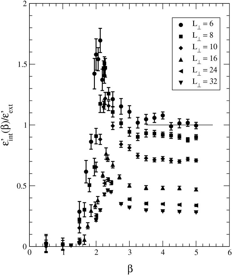
Figure 1: The $\beta$-derivative of the internal energy density Eq. (4.5) versus $\beta$ at different values of the transverse lattice size $L_{\perp}$.

In Figure 1 we display the derivative of the energy density normalized to the derivative of the external energy density:

$$\varepsilon^{\prime}_{\mathrm{ext}}=1-\cos(\frac{gH}{2})=1-\cos(\frac{2\pi}{L_{1}}n_{\mathrm{ext}})$$ (4.6)

versus $\beta$ for $L_{1}=L_{4}=32$ and $6\leq L_{\perp}\leq 32$. From Figure 1 we see that in the strong coupling region $\beta\lesssim 1$ the external background field is completely shielded. Moreover $\varepsilon^{\prime}_{\mathrm{int}}$ display a peak at $\beta\simeq 2.2$ resembling the behavior of the specific heat [18, 19]. This is not surprising since our previous studies [20] in U(1) showed that $\varepsilon^{\prime}_{\mathrm{int}}$ behaves like a specific heat.

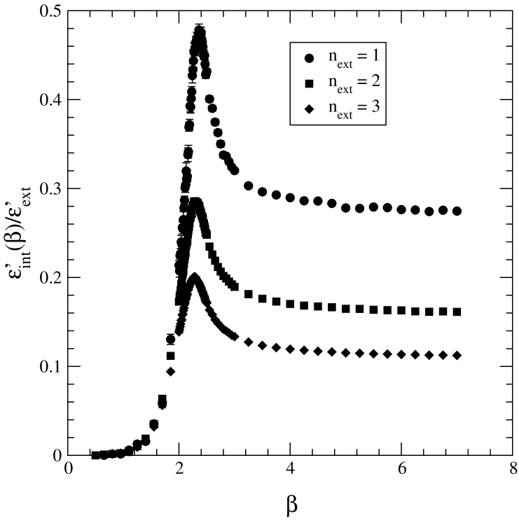
Figure 2: The $\beta$-derivative of the internal energy density Eq. (4.5) versus $\beta$ for a transverse lattice size $L_{\perp}=32$ at different values of applied external field strength.

In the weak coupling region $\beta\gtrsim 3$ Fig. 1 shows that the ratio $\varepsilon^{\prime}_{\mathrm{int}}/\varepsilon^{\prime}_{\mathrm{ext}}$ stays constant. Actually the constant does depend on $L_{\perp}$ and $n_{\mathrm{ext}}$. Indeed in Fig. 1 the dependence on $L_{\perp}$ for fixed external magnetic field is evident. On the other hand in Fig. 2 we keep $L_{\perp}=32$ fixed and vary $n_{\mathrm{ext}}$. We see clearly that the weak coupling plateau decreases by increasing the external field. In order to extract $\varepsilon_{\mathrm{int}}(\beta,n_{\mathrm{ext}})$ we can numerically integrate the data for $\varepsilon^{\prime}_{\mathrm{int}}(\beta,n_{\mathrm{ext}})/\varepsilon^{\prime}_{\mathrm{ext}}$ using the trapezoidal rule

$$\varepsilon_{\mathrm{int}}(\beta,n_{\mathrm{ext}})=\varepsilon^{\prime}_{\mathrm{ext}}\,\int_{0}^{\beta}\frac{\varepsilon^{\prime}_{\mathrm{int}}(\beta,n_{\mathrm{ext}})}{\varepsilon^{\prime}_{\mathrm{ext}}}\,d\beta^{\prime}\,.$$ (4.7)

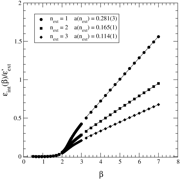
Figure 3: The energy density Eq. (4.7) versus $\beta$ for transverse lattice size $L_{\perp}=32$ at different values of applied external field strength. The solid lines are the linear fits Eq. (4.8).

In Figure 3 we display $\varepsilon_{\mathrm{int}}(\beta,n_{\mathrm{ext}})$ obtained from Eq. (4.7). The plateau of the derivative of the internal energy density in the weak coupling region results in a linear rising term in the energy density. For $\beta\gg 1$ we get

$$\varepsilon_{\mathrm{int}}(\beta,n_{\mathrm{ext}})\simeq\beta\varepsilon^{\prime}_{\mathrm{ext}}a(n_{\mathrm{ext}})\,.$$ (4.8)

Moreover for $\beta\gg 1$ we get also

$$\beta\,\varepsilon^{\prime}_{\mathrm{int}}=\beta\,(1-\cos\frac{2\pi}{L_{1}}n_{\mathrm{ext}})\simeq\frac{1}{2}H^{2}\,.$$ (4.9)

So that in the weak coupling region

$$\varepsilon_{\mathrm{int}}(\beta,n_{\mathrm{ext}})\simeq a(n_{\mathrm{ext}})\frac{1}{2}H^{2}\,,\quad\beta\gg 1\,.$$ (4.10)

Figure 1 shows that $a(n_{\mathrm{ext}})\simeq 1$ for $L_{\perp}\simeq 6-8$ and $n_{\mathrm{ext}}=1$. On the other hand $a(n_{\mathrm{ext}})$ decreases by increasing $L_{\perp}$ or the external background field. This peculiar behavior can be compared with the Abelian case where we found that $a(n_{\mathrm{ext}})\simeq 1$ independently on $L_{\perp}$ and $n_{\mathrm{ext}}$ [9, 20]. Previous theoretical studies [15] suggested that due to the presence of the Nielsen-Olesen modes the gauge system reacts strongly to the external perturbation even in the nominally perturbative regime. It turns out that the Nielsen-Olesen modes behave like a (1+1)-dimensional tachionic charged scalar field. The condensation of these modes takes place only in the thermodynamic limit. As a consequence the applied external background magnetic field is almost completely screened and there is a dramatic reduction of the vacuum magnetic energy. Indeed it turns out that in the infinite volume limit the perturbative vacuum and the magnetic condensate vacuum are degenerate for vanishing gauge coupling.

On the lattice the Nielsen-Olesen modes display the one-loop instability when $\lambda_{u}$ given by Eq. (3.51) becomes negative. In the approximation adopted in Sect. III we find that $\lambda_{u}$ gets negative by increasing $L_{\perp}$ for fixed external field. Thus we can switch on and off the one-loop instability by varying $L_{\perp}$. This has been also noticed by the Authors of Ref. [21]. For instance, by using Eqs. (2.4), (3.33), and (3.51) with $L_{1}=L_{4}=32$ and $n_{\mathrm{ext}}=1$ we find that $\lambda_{u}\lesssim 0$ for $L_{\perp}\gtrsim 11$.

Our numerical results in Fig. 1 show that for $n_{\mathrm{ext}}=1$ and $L_{\perp}\lesssim 10$ there is no the Nielsen-Olesen instability and the gauge system responds weakly to the external perturbation in the weak coupling region. On the other hand, by increasing $L_{\perp}$ (see Fig. 1) or $n_{\mathrm{ext}}$ (see Fig. 2) we increment the lattice Nielsen-Olesen modes. As a consequence we find a clear reduction of the vacuum energy density for both the peak values of $\varepsilon^{\prime}_{\mathrm{int}}(\beta,n_{\mathrm{ext}})$ and the coefficient $a(n_{\mathrm{ext}})$ in Eq. (4.10) decreases towards zero in the thermodynamic limit. To see this we need to perform the infinite volume extrapolation. We can extract more information from our numerical data by expressing them versus

$$x=\frac{a_{H}}{L_{\mathrm{eff}}}\,,$$ (4.11)

where

$$a_{H}=\sqrt{\frac{2\pi}{gH}}=\sqrt{\frac{L_{1}}{2n_{\mathrm{ext}}}}$$ (4.12)

is the magnetic length and

$$L_{\mathrm{eff}}=\Omega_{\mathrm{int}}^{1/4}$$ (4.13)

is the lattice effective linear size. Indeed we find that the data for $\varepsilon^{\prime}_{\mathrm{int}}(\beta,n_{\mathrm{ext}})/\varepsilon^{\prime}_{\mathrm{ext}}$ at the perturbative tail and at the peak for various lattice sizes and values of $n_{\mathrm{ext}}$ can be expressed as a function of the scaling variable $x$ (defined in Eq. (4.11)):

$$\frac{\varepsilon^{\prime}_{\mathrm{int}}(\beta,n_{\mathrm{ext}})}{\varepsilon^{\prime}_{\mathrm{ext}}}=\kappa(\beta)x^{\alpha}\,.$$ (4.14)

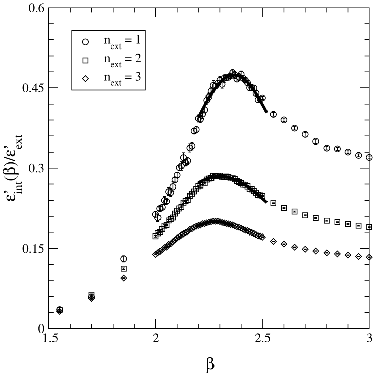
Figure 4: The data displayed in Fig. 2 near the peaks of the $\beta$-derivative of the internal energy density Eq. (4.5) in correspondence of each value of $n_{\mathrm{ext}}$. The solid lines are the fits Eq. (4.15).

For the perturbative tail of $\varepsilon^{\prime}_{\mathrm{int}}(\beta,n_{\mathrm{ext}})/\varepsilon^{\prime}_{\mathrm{ext}}$ we keep the value of the ratio at $\beta=5$. On the other hand, the peak values have been extracted by fitting the values around the peak to (see Fig. 4)

$$\frac{\varepsilon^{\prime}_{\mathrm{int}}(\beta,n_{\mathrm{ext}})}{\varepsilon^{\prime}_{\mathrm{ext}}}=\frac{a_{1}}{a_{2}(\beta-\beta_{\mathrm{peak}})^{2}+1}\,.$$ (4.15)

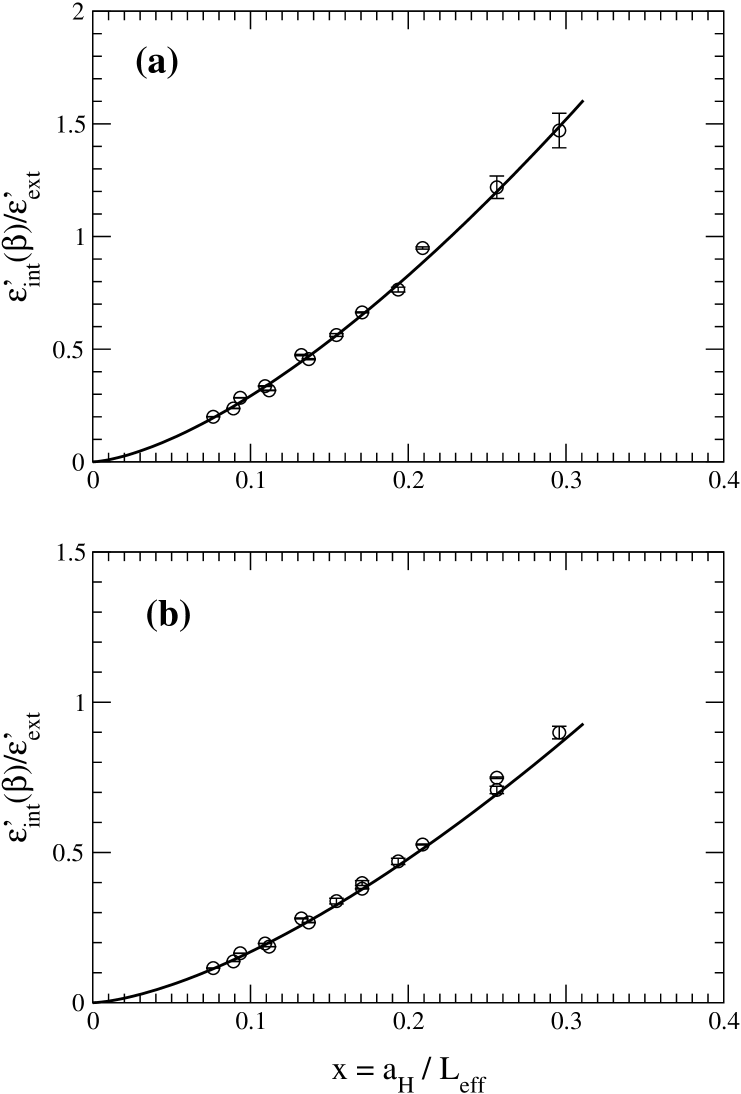
Figure 5: The lattice data for $\varepsilon^{\prime}_{\mathrm{int}}(\beta,n_{\mathrm{ext}})/\varepsilon^{\prime}_{\mathrm{ext}}$ at different values of the transverse lattice size $L_{\perp}$ and external field strength $n_{\mathrm{ext}}$ for $\beta=5$ (a) and $\beta=\beta_{\mathrm{peak}}$ (b), versus the scaling variable defined in Eq. (4.11). The solid lines are the fits Eq. (4.14) with $\alpha=1.5$.

From Eq. (4.15) we extract the peak value, $a_{1}$, and the peak position $\beta_{\mathrm{peak}}$. It has been found that the data are compatible with the scaling law Eq. (4.14) with $\alpha=1.5$ (see Fig. 5). It is remarkable that the same power-law arises if we adopt the alternative boundary conditions given by Eq. (2.5). So that we see that both boundary conditions Eq. (2.3) or Eq. (2.5) lead to the same thermodynamic limit.

If we, further, take into account the shifts $\Delta\beta$ of the peak values, that turns out to depend only on $n_{\mathrm{ext}}$, we are led to the universal scaling-law

$$x^{-\alpha}\frac{\varepsilon^{\prime}_{\mathrm{int}}(\tilde{\beta},n_{\mathrm{ext}},L_{\mathrm{eff}})}{\varepsilon^{\prime}_{\mathrm{ext}}}=\kappa(\tilde{\beta})\,,$$ (4.16)

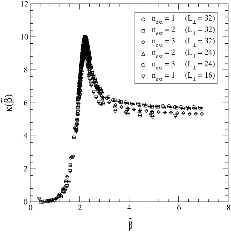
Figure 6: The scaling curve obtained by re-scaling all lattice data for $\varepsilon^{\prime}_{\mathrm{int}}(\tilde{\beta},n_{\mathrm{ext}},L_{\mathrm{eff}})$ according to Eq. (4.16).

where $\tilde{\beta}=\beta-\Delta\beta$. Indeed Figure 6 shows that all our numerical data (for all the values of $a_{H}$ and $L_{\mathrm{eff}}$) can be approximately arranged on the scaling curve $\kappa(\beta)$. Remarkably we find that the peak in $\kappa(\beta)$ is located at $\beta_{c}=2.2209(68)$ which agrees with the peak position of the specific heat extrapolated to the infinite volume limit $\beta_{c}=2.23(2)$ [19]. By using Eq.(4.16) we can determine the infinite volume limit of the vacuum energy density $\varepsilon_{\mathrm{int}}$. We have

$$\lim_{L_{\mathrm{eff}}\to\infty}\varepsilon_{\mathrm{int}}(\beta,n_{\mathrm{ext}},L_{\mathrm{eff}})=\varepsilon^{\prime}_{\mathrm{ext}}\,\int_{0}^{\tilde{\beta}}d{\tilde{\beta^{\prime}}}\,\kappa(\tilde{\beta^{\prime}})$$ (4.17)

$$\qquad\qquad\qquad\qquad\qquad\qquad\times\lim_{L_{\mathrm{eff}}\to\infty}\left(\frac{a_{H}}{L_{\mathrm{eff}}}\right)^{\alpha}$$

$$\simeq\frac{H^{2}}{2\beta}\left[\int_{0}^{\tilde{\beta}}d{\tilde{\beta^{\prime}}}\,\kappa(\tilde{\beta^{\prime}})\right]\times\lim_{L_{\mathrm{eff}}\to\infty}\left(\frac{a_{H}}{L_{\mathrm{eff}}}\right)^{\alpha}=0\,,$$

in the whole range of $\beta$. This in turn implies that in the continuum limit $(L_{\mathrm{eff}}\to\infty,\beta\to\infty)$ the SU(2) vacuum completely screens the external chromomagnetic Abelian field. In other words, the continuum vacuum behaves as an Abelian magnetic condensate medium in accordance with the dual superconductivity scenario.

V. MONTE CARLO SIMULATIONS: $T\neq 0$

We can extend the study of the SU(2) gauge system in an external chromomagnetic Abelian field to the case of finite temperature. As it is well known the relevant dynamical quantity is the free energy. On the lattice the physical temperature $T_{\mathrm{phys}}$ is introduced by (in units of $\kappa_{B}=1$):

$$\frac{1}{T_{\mathrm{phys}}}=L_{t}\cdot a\,,$$ (5.1)

where $L_{t}$ is the linear extension in the time direction $L_{t}=L_{4}$, while the extension on the spatial direction should be infinite. In numerical simulations, however, the spatial extension would of course be finite. In order to approximate the thermodynamic limit one should respect the relation

$$L_{s}\gg L_{t}\,.$$ (5.2)

We perform our numerical simulation on $32^{3}\times L_{t}$ lattices by imposing

$$\frac{L_{t}}{L_{s}}\leq 4$$ (5.3)

in order to avoid finite volume effects.

In the case of constant external chromomagnetic field the relevant quantity is the density of the free energy

$$F[\vec{A}^{\mathrm{ext}}]=-\frac{1}{VL_{t}}\ln\frac{\mathcal{Z}[\vec{A}^{\mathrm{ext}}]}{{\mathcal{Z}}[0]}\,,\quad V=L_{s}^{3}\,.$$ (5.4)

The pure gauge system undergoes the deconfinement phase transition by increasing the temperature. The order parameter for the deconfinement phase transition is the Polyakov loop

$$P={\mathrm{Tr}}\prod_{x_{4}=1}^{L_{t}}U_{4}(x)\,.$$ (5.5)

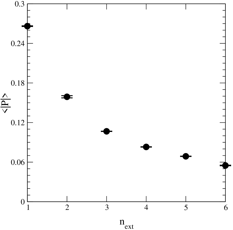
Figure 7: The absolute value of the Polyakov loop on a $32^{3}\times 5$ lattice at $\beta=2.5$ versus $n_{\mathrm{ext}}$.

As a preliminary step we look at the behavior of the temporal Polyakov loop $\langle P\rangle$ versus the external applied field. We start with the SU(2) gauge system at $\beta=2.5$ on $32^{3}\times 5$ lattice at zero applied external field (i.e. $n_{\mathrm{ext}}=0$) that is known to be in the deconfined phase of finite temperature SU(2). If the external field strength is increased the expectation value of the Polyakov loop is driven towards the value at zero temperature (see Fig. 7). Similar behavior has been reported by the authors of Ref. [22] within a different approach. It is worthwhile to stress that our result is consistent with the dual superconductor mechanism of confinement.

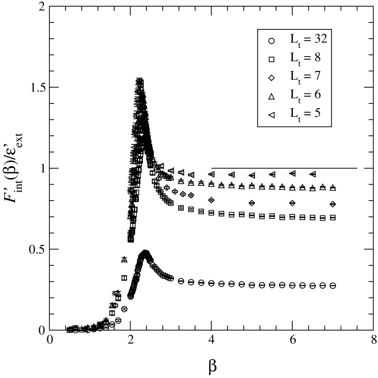
Figure 8: The $\beta$-derivative of the free energy density Eq. (5.4) $F^{\prime}_{\mathrm{int}}(\beta,n_{\mathrm{ext}})/\varepsilon^{\prime}_{\mathrm{ext}}$ versus $\beta$ at different values of the temporal lattice extension $L_{t}$.

On the other hand, if we start with the SU(2) gauge system at zero temperature in a constant Abelian chromomagnetic background field of fixed strength ($n_{\mathrm{ext}}=1$) and increase the temperature, then we find that the perturbative tail of the $\beta$-derivative of the free energy density $F^{\prime}_{\mathrm{int}}(\beta,n_{\mathrm{ext}})/\varepsilon^{\prime}_{\mathrm{ext}}$ increases with $1/L_{t}$ and tends towards the “classical” value $F^{\prime}_{\mathrm{int}}(\beta,n_{\mathrm{ext}})/\varepsilon^{\prime}_{\mathrm{ext}}\simeq 1$ (see Fig. 8).

We may conclude, then, that by increasing the temperature there is no screening effect in the free energy density confirming that the zero-temperature screening of the external field is related to the confinement. Moreover the information of $F^{\prime}_{\mathrm{int}}(\beta,n_{\mathrm{ext}})/\varepsilon^{\prime}_{\mathrm{ext}}$ at finite temperature can be used to get an estimate of the deconfinement temperature $T_{c}$. In Figure 9 we magnify the peak region for various values of $L_{t}$. We see clearly that the pseudocritical coupling $\beta^{*}(L_{t})$ depends on $L_{t}$. To determine the pseudocritical couplings we parametrize $F^{\prime}_{\mathrm{int}}(\beta,L_{t})$ near the peak as

$$\frac{F^{\prime}_{\mathrm{int}}(\beta,L_{t})}{\varepsilon^{\prime}_{\mathrm{ext}}}=\frac{a_{1}(L_{t})}{a_{2}(L_{t})[\beta-\beta^{*}(L_{t})]^{2}+1}\,.$$ (5.6)

We restrict the region near $\beta^{*}(L_{t})$ until the fits Eq. (5.6) give a reduced $\chi^{2}$ of order $1$.

Having determined $\beta^{*}(L_{t})$ we estimate the deconfinement temperature as

$$\frac{T_{c}}{\Lambda_{\mathrm{latt}}}=\frac{1}{L_{t}-1}\frac{1}{f(\beta^{*}(L_{t}))}\,,$$ (5.7)

where

$$f(\beta)=\left(\frac{11}{6\pi^{2}}\frac{1}{\beta}\right)^{-51/121}\,\exp(-\frac{3\pi^{2}}{11}\beta)\,.$$ (5.8)

In Eq.( 5.7) we take into account that, due to the frozen time slice, the effective extension in the time direction is $L_{t}^{\mathrm{eff}}=L_{t}-1$.

In Figure 10 we display $T_{c}/\Lambda_{\mathrm{latt}}$ for different temperatures. Following Ref. [23] we perform a linear extrapolation to the continuum of our data for $T_{c}/\Lambda_{\mathrm{latt}}$. We see that our estimate of $T_{c}/\Lambda_{\mathrm{latt}}$ in the continuum is in fair agreement with the one available in the literature [23]:

$$\frac{T_{c}}{\Lambda_{\mathrm{latt}}}=24.38\pm 2.18\,.$$ (5.9)

VI. CONCLUSIONS

We have studied the non-perturbative dynamics of the vacuum of SU(2) lattice gauge theory by means of the gauge-invariant effective action defined using the lattice Schrödinger functional.

At zero temperature our numerical results indicate that in the continuum limit $L_{\mathrm{eff}}\to\infty$, $\beta\to\infty$ we have

$$\varepsilon[\vec{A}^{\mathrm{ext}}]=0\,,$$ (6.1)

so that the vacuum screens completely the external chromomagnetic Abelian field. In other words, the continuum vacuum behaves as an Abelian magnetic condensate medium in accordance with the dual superconductivity scenario. In particular we have

$$\varepsilon[\vec{A}^{\mathrm{ext}}]\sim H^{a}_{k}B^{a}_{k}=\frac{1}{\mu}F^{a}_{ij}F^{a}_{ij}\,$$ (6.2)

where $\mu$ is the vacuum color magnetic permeability. Thus Eq. (6.1) implies that $\mu\to\infty$ in the continuum limit. As a consequence by Lorentz invariance the vacuum color dielectric constant tends to zero. This in turns implies that the vacuum does not support an isolated color charge, i.e. the color confinement.

The intimate connection between the screening of the external background field and the confinement is corroborated by the finite temperature results. Indeed our numerical data show that the zero-temperature screening of the external field is removed by increasing the temperature. Moreover, at finite temperature it seems that confinement is restored by increasing the strength of the external applied field.

At finite temperature we find that the $\beta$-derivative of the free energy density behaves like a specific heat. From the peak position of the $\beta$-derivative of the free energy density we obtained an estimation of the critical temperature $T_{c}/\Lambda_{\mathrm{latt}}$ that extrapolates in the continuum limit to a value consistent with previous determinations in the literature.

Let us conclude by stressing that our method can be easily extended to the SU(3) gauge theory. Moreover we also feel that the lattice gauge invariant effective action could be also employed to study different background fields.

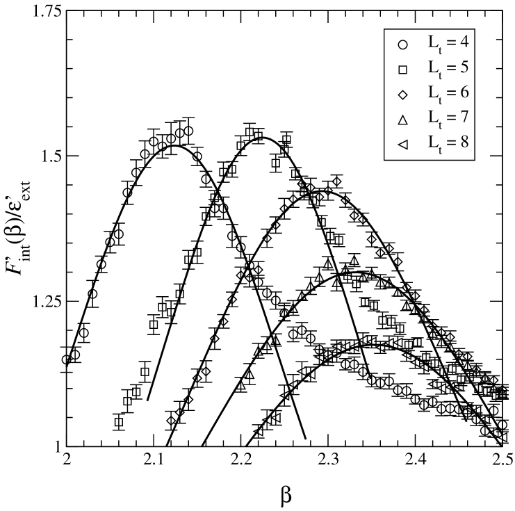
Figure 9: The peak region for various values of $L_{t}$. The solid lines are the fits Eq. (5.6).

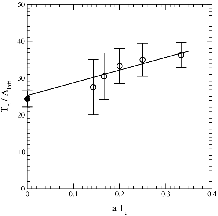
Figure 10: Our lattice data for $T_{c}/\Lambda_{\mathrm{latt}}$ versus the temperature (circles). The full circle is the continuum estrapolation of Ref. [23] (see Eq. (5.9)). The solid line is a linear fit to our data.

References

- [1] J. Schwinger, Phys. Rev. 82, 664 (1951).
- [2] J. Honerkamp, Nucl. Phys. B36, 130 (1971); Nucl. Phys. B48, 269 (1972).
- [3] G. ’t Hooft, Nucl. Phys. B62, 444 (1973).
- [4] P. Cea and L. Cosmai, Phys. Rev. D48, 3364 (1993); Nucl. Phys. Proc. Suppl. 34, 234 (1994); hep-lat/9306007.
- [5] H. D. Trottier and R. M. Woloshyn, Phys. Rev. Lett. 70, 2053 (1993); Phys. Rev. Lett. 72, 4155 (1994).
- [6] P. Cea and L. Cosmai, Phys. Rev. D43, 620 (1991); Phys. Lett. B264 415 (1991).
- [7] J. Ambjorn, V.K. Mitryushkin, and V.G. Bornyakov, Phys. Lett. B225, 153 (1989); Phys. Lett. B245, 575 (1990).
- [8] A. R. Levi, Nucl. Phys. Proc. Suppl. 34, 161 (1994).
- [9] P. Cea, L. Cosmai, and A.D. Polosa, Phys. Lett. B392, 177 (1997).
- [10] G.C. Rossi and M. Testa, Nucl. Phys. B163, 109 (1980); Nucl. Phys. B176, 477 (1980). For a recent review see: G. C. Rossi, hep-th/9810177.
- [11] D. J. Gross, R. D. Pisarski, and L. G. Yaffe, Rev. Mod. Phys. 53, 43 (1981).
- [12] M. Lüscher, R. Narayanan, P. Weisz, and U. Wolff, Nucl. Phys. B384, 168 (1992); M. Lüscher and P. Weisz, Nucl. Phys. B452, 213 (1995).
- [13] A partial account of the results of the present paper appeared in P. Cea and L. Cosmai, Mod. Phys. Lett. A13, 861 (1998); hep-lat/9809042.
- [14] N. K. Nielsen and P. Olesen, Nucl. Phys. B144, 376 (1978).
- [15] P. Cea, Phys. Rev. D37, 1637 (1988).
- [16] R. Dashen and D. J. Gross, Phys. Rev. D23, 2340 (1981).
- [17] A. Hasenfratz, P. Hasenfratz, and F. Niedermeyer, Nucl. Phys. B329, 739 (1990).
- [18] B. Lautrup and M. Nauenberg, Phys. Rev. Lett. 45, 1755 (1980);
- [19] J. Engels and T. Scheideler, Nucl. Phys. Proc. Suppl. 53, 423 (1997).
- [20] P. Cea, L. Cosmai, and A. D. Polosa, Phys. Lett. B397, 229 (1997).
- [21] A.R. Levi and J. Polonyi, Phys. Lett. B357, 186 (1995).
- [22] P. N. Meisinger and M. C. Ogilvie, Phys. Lett. B407, 297 (1997); M. C. Ogilvie, Nucl. Phys. Proc. Suppl. 63, 430 (1998).
- [23] J. Fingberg, U. Heller, F. Karsch, Nucl. Phys. B392 (1993) 493.