End states, ladder compounds, and domain wall fermions

Abstract

A magnetic field applied to a cross linked ladder compound can generate isolated electronic states bound to the ends of the chain. After exploring the interference phenomena responsible, I discuss a connection to the domain wall approach to chiral fermions in lattice gauge theory. The robust nature of the states under small variations of the bond strengths is tied to chiral symmetry and the multiplicative renormalization of fermion masses.

Isolated electronic states can appear when a magnetic field is applied to a ladder system with diagonal cross linking. The basic structure is shown in Fig. 1. A single electron inserted in such a system will hop around and, with dissipation, settle into a ground state with wave function non-vanishing on all sites. When a magnetic field is present, phases appear which can cause interesting interference effects. In special cases this results in unusual states that do not diffuse through the system, but instead are bound to the ends of the chain. When the field has a strength of half a flux unit per plaquette, symmetries exactly determine the energy of these special states.

These end states are a particular manifestation of the surface states discussed by Shockley [1]. They are presumably also a one dimensional remnant of the edge states discussed in Ref. [2]. My entire treatment is in terms of free fermions hopping through the fixed lattice; I include no four fermion interactions.

On the promotion of the system to a five space-time dimensional model with appropriate spin factors, these states become precisely the chiral modes of the Kaplan-Furman-Shamir [3] domain-wall fermions currently being used [4] in lattice gauge simulations. My goal here is a qualitative picture for the chiral nature of these surface modes.

I start with a spin-less electron on the basic structure of Fig. 1. All horizontal bonds are of equal strength, given by hopping parameter $K$. For vertical bonds, the coupling is $M$ and for the diagonal bonds $Kr$. I assume these parameters are positive. The notation is motivated by the later connection with lattice gauge models. Thus my starting Hamiltonian is

$$H=-\sum_{n}\bigg{(} K(a_{n}^{\dagger}a_{n+1}+a_{n+1}^{\dagger}a_{n}+b_{n}^{\dagger}b_{n+1}+b_{n+1}^{\dagger}b_{n})$$ (3)

$$+Kr(a_{n}^{\dagger}b_{n+1}+b_{n+1}^{\dagger}a_{n}+b_{n}^{\dagger}a_{n+1}+a_{n+1}^{\dagger}b_{n})$$

$$+M(a_{n}^{\dagger}b_{n}+b_{n}^{\dagger}a_{n})\bigg{)}$$

where $a_{n}$ and $b_{n}$ are fermionic annihilation operators on the $n$’th site of the upper and lower chains, respectively. A general one particle state is

$$|\chi\rangle=\sum_{n=1}^{L}\pmatrix{a_{n}^{\dagger}&b_{n}^{\dagger}\cr}\pmatrix{\psi^{a}_{n}\cr\psi^{b}_{n}}|0\rangle$$ (4)

Here $|0\rangle$ represents the bare vacuum with no fermions present.

For an infinite chain this model is easily solved via Fourier transform

$$H=-\int_{0}^{2\pi}{dq\over 2\pi}\pmatrix{\tilde{a}_{q}^{\dagger}&\tilde{b}_{q}^{\dagger}\cr}\pmatrix{2K\cos(q)&M+2Kr\cos(q)\cr M+2Kr\cos(q)&2K\cos(q)\cr}\pmatrix{\tilde{a}_{q}\cr\tilde{b}_{q}\cr}$$ (5)

where $\tilde{a}_{q}=\sum_{n}a_{n}e^{iqx}$. Thus the energy eigenvalues are

$$E_{\pm}(q)=-2K\cos(q)\pm\left(M+2Kr\cos(q)\right)$$ (6)

Generically, two bands correspond to even and odd states under inversion of the system around the horizontal axis. Depending on parameters, these bands may or may not overlap. Here I am interested in the small $M/K$ case, where they do overlap. These momentum space solutions carry over to a finite periodic system of length $L$, except with discrete values for the momentum, $q=2\pi n/L$, $n$ an integer.

Now apply a perpendicular magnetic field. This induces phases when a particle hops around closed loops. The details are gauge dependent; I adopt the convention of placing these factors on the upper and lower horizontal bonds, generalizing my Hamiltonian to

$$H=-\sum_{n}\bigg{(} K(e^{i\theta}a_{n}^{\dagger}a_{n+1}+e^{-i\theta}a_{n+1}^{\dagger}a_{n}+e^{-i\theta}b_{n}^{\dagger}b_{n+1}+e^{i\theta}b_{n+1}^{\dagger}b_{n})$$ (9)

$$+Kr(a_{n}^{\dagger}b_{n+1}+b_{n+1}^{\dagger}a_{n}+b_{n}^{\dagger}a_{n+1}+a_{n+1}^{\dagger}b_{n})$$

$$+M(a_{n}^{\dagger}b_{n}+b_{n}^{\dagger}a_{n})\bigg{)}$$

In natural units, the magnetic flux is $\theta/\pi$ through each plaquette. Eq. 5 now becomes

$$H=-\int_{0}^{2\pi}{dq\over 2\pi}\pmatrix{\tilde{a}_{q}^{\dagger}&\tilde{b}_{q}^{\dagger}\cr}\pmatrix{2K\cos(q-\theta)&M+2Kr\cos(q)\cr M+2Kr\cos(q)&2K\cos(q+\theta)\cr}\pmatrix{\tilde{a}_{q}\cr\tilde{b}_{q}\cr}$$ (10)

and the energy eigenvalues are

$$E_{\pm}(q)=-2K\cos(q)\cos(\theta)\pm\sqrt{4K^{2}\sin^{2}(q)\sin^{2}(\theta)+(M+2Kr\cos(q))^{2}}$$ (11)

For sufficient field, the two bands can separate, leaving a gap in the spectrum. For small $M/2Kr$, this opening can produce the situation discussed in Ref. [1]. For small $r$ the lower band has its maximum at $q=\pi$, the upper band has its minimum at $q=0$ and the band separation occurs at $\theta=\cos^{-1}(r)$. For large $r$, the separation of the bands occurs at momentum $q=\pi-\cos^{-1}(M/2Kr)$, as soon as the field is present.

A particularly interesting limit occurs for half a flux unit per plaquette, i.e. $\theta=\pi/2$. These relative phases are sketched in Fig. 1. The cancellations are most dramatic when $M=0$ and $r=1$, i.e. no vertical bonds and all others equal in magnitude. Then all paths from a given site to any location two or more sites away cancel, as illustrated in Fig. 2. Electrons cannot diffuse throughout the system. Eq. 11 reduces to all states having either energy $2K$ or $-2K$. With constant energies, group velocities vanish and nothing moves. For explicit solutions, consider a given site $n$ and the (unnormalized) wave function with $\psi_{n}=\pmatrix{i\cr 1\cr}$, $\psi_{n+1}=\pm\pmatrix{1\cr i\cr}$ and all other $\psi_{j}=0$. These soliton like states have energy $\mp 2K$, respectively and are locked onto the plaquette between site $n$ and $n+1$. As there are two solutions for every plaquette and there twice as many atoms as plaquettes, this is a complete set of states for either the infinite or the periodic case.

Now suppose we have not a periodic but a finite open system. Let the sites (each with two atoms) run over the range $1\leq n\leq L$. Open boundaries means no direct connection from site $L$ back to site $1$. For the moment, I stay with the above special case with $\theta=\pi/2$, $M=0$ and $r=1$. Now there is one more site than the number of plaquettes, and therefore two more states than the above solitons. One of these states has

$$\matrix{&\psi_{1}=\pmatrix{1\cr i\cr}\cr&\psi_{n}=0\qquad n\neq 1\cr}$$ (12)

The electron cannot hop anywhere because all such attempts interfere completely. It is locked onto the end of the chain. This state is time independent; it has exactly zero energy. A symmetric state binds to the other end of the system, with

$$\matrix{&\psi_{L}=\pmatrix{i\cr 1\cr}\cr&\psi_{n}=0\qquad n\neq L\cr}$$ (13)

These two states are related by rotating by $\pi$ about the axis of the magnetic field.

Now move away from the special case with $M=0$ and $r=1$. Then the upper and lower bands broaden and the above solitonic states mix and move. By continuity, however, the end states cannot suddenly disappear. They are robust under small variations of the parameters. Keeping $\theta=\pi/2$ and considering the long $L$ limit, symmetries force these modes to remain at zero energy. Rotating the system by $\pi$ about the the magnetic field interchanges them; thus they have equal energy. However, redefining all the $b$ operators to include a minus sign, i.e. $b_{n}\rightarrow-b_{n}$, and then swapping the ends of the system with $n\rightarrow L-n+1$ takes the Hamiltonian into its negative. This requires the energies to be of opposite sign. In particle physics language, the energies are protected from renormalization. This is reminiscent of the role of chiral symmetry in continuum field theories, and is the basis of the domain wall analogy discussed below.

This restriction on the energies weakens when the magnetic field strength varies. The left-right symmetry keeps the states degenerate, but no longer necessarily at zero energy. As the field is reduced, generically the states drift until pinched between the bands of the full system. For the remainder of this discussion I keep $\theta=\pi/2$, and the end states remain at zero energy. While taking $(M,r)=(0,1)$ seems to avoid the requirement of a large $L$ limit, this is not robust. Indeed, to avoid doublers, these parameters become functions of physical momenta when I later extend the model to higher dimensions.

To be more explicit, consider small $M$, keeping $\theta=\pi/2$ and $r=1$. Then the solution remains quite simple in the large $L$ limit, i.e. for a semi-infinite chain we have the (unnormalized) wave function

$$\psi_{n}=(-M/2)^{n}\pmatrix{1\cr i\cr},$$ (14)

sketched in Fig. 3 for $M=1$. The modes extend into the chain with an exponential falloff. Note that when $M$ gets too large, i.e. at $M=2$, the modes are lost. At this point the wave function is no longer damped, and the modes are absorbed into the continuous bands. This is also the point at which the band gap vanishes. Finally, for finite $L$ these modes feel the opposite ends of the system. Generically a small mixing, exponentially suppressed with the length $L$, drives them from exactly zero energy.

Varying $r$ preserves the modes as well, although the resulting wave function becomes a bit more complicated. Although the notation is different, the following discussion is essentially equivalent to arguments in Ref. [5]. The desired solution is the superposition of two eigenstates under translation along the lattice. The boundary condition for the wave function to vanish at site 0 can be guaranteed with the form

$$\psi_{n}={\lambda_{1}^{n}-\lambda_{2}^{n}\over\lambda_{1}-\lambda_{2}}\psi_{1}$$ (15)

Thus we need the peculiar situation of two different translation eigenvalues with the same eigenvector. At zero energy the basic requirement for a translation eigenvalue is

$$\pmatrix{-i(1-\lambda^{2})&r(1+\lambda^{2})+(M/K)\lambda\cr r(1+\lambda^{2})+(M/K)\lambda&i(1-\lambda^{2})\cr}\psi=0$$ (16)

Then $\psi=\pmatrix{1\cr i\cr}$ is an eigenvector for both solutions of the quadratic equation

$$r(1+\lambda^{2})+(M/K)\lambda=1-\lambda^{2}$$ (17)

These two solutions are

$$\lambda_{1,2}={-M\pm\sqrt{M^{2}+4K^{2}(1-r^{2})}\over 2K(1+r)}$$ (18)

For small $M$ and $r$ near one, both roots are less than unity in magnitude, required for the end state to be normalizable. For the opposite end of the chain, we use $\psi=\pmatrix{i\cr 1\cr}$, which gives solutions which are the inverse of those in Eq. 18.

When $r=1$, one eigenvalue vanishes, giving the simple exponential form in Eq. 14. When $M=0$ as well, both eigenvalues vanish, and the state adheres to a single end site. If we change the magnetic field so $\theta\neq\pi/2$, then the energy needs to be adjusted to keep the two eigenvalues with the same eigenvector. This is automatic at zero energy when $\theta=\pi/2$. The end states cease to exist when one of the eigenvalues becomes unity in magnitude, i.e. when

$$M=2Kr.$$ (19)

For larger $M$ the zero modes are absorbed into the continuum bands.

I now turn to some interesting effects when several of these chains are connected at a “junction.” First note that this simple cross linked ladder system can have excitations which only move one direction, backing themselves up into end states. Start in a state with all negative energy levels filled and all others empty. This is just shy of half filled because the end states are empty. Now insert an electron wave packet with wave function $\psi_{n}\sim\pmatrix{1\cr i\cr}$ by applying a superposition of the operators $\pmatrix{a_{n}^{\dagger}&b_{n}^{\dagger}\cr}\pmatrix{1\cr i\cr}$ to the nearly half filled system.

Because of the phase cancellations, this wave packet initially spreads only to the left. It is a mixture of the left end state and positive energy states, which are effectively plane waves. As constructed, the state has no overlap with the right end state. If we add a damping to the positive energy modes, the electron will ultimately settle into the left edge state.

Now join three such ladders. Fig. 4 sketches a connection of the earlier ladder onto the side of another. I refer to the horizontal chain in this figure as the side chain, and the one in the indicated $z$ direction as the main chain. Now release a left moving electron on the side chain as discussed above. As the state approaches the junction, it will turn in the direction dictated by the phases on the main chain. Asymptotically the electron moves to only one end of the main chain.

At this point I can make a rather interesting device by generalizing the model to two component spinors on each atom. Put a Pauli matrix, say $\sigma_{3}$, onto the horizontal bonds on the main chain. I put no extra factors on the side chain. When the particle meets the junction from the side chain, spin determines the direction it turns. I have a spin separator. If the chain lies in the same physical direction as the Pauli matrix, it is a helicity filter. This situation is sketched in Fig. 4. This is the link to chiral symmetry.

The above picture is at the heart of the domain wall formulation of chiral fermions. To map this discussion onto the latter, one ladder molecule is placed at every site of a three dimensional space lattice. The system is then half filled, setting the Fermi surface at the level of the zero modes. Next, to allow motion in the physical directions, additional hopping terms couple different sites. For the standard picture, corresponding atoms on neighboring space sites are coupled.

To connect with the usual language, the distance along the ladders represents a “fifth” dimension. The Dirac matrices of the four dimensional theory become the Pauli matrices inserted in the “device” discussed above. The spin separation of the surface modes corresponds to their chiral nature. Since this is a Hamiltonian discussion, I treat time as a continuous variable [5]. Standard techniques relate this model to the Lagrangian path integral [6].

On this higher dimensional system, the end states become surface modes, representing the light Fermions of the physical world. As in Fig. 4, on each surface these modes have their helicity projected. The separation of spin modes corresponds to chiral symmetry. The particle energies also receive a contribution from momentum in the physical directions. The symmetries force zero momentum states to zero energy; we have naturally massless particles. Interactions which renormalize the relative bond strengths will not change this; any mass renormalization must be proportional to explicit mass terms.

My phase conventions correspond to a particular representation for the Dirac gamma matrices. In conventional lattice gauge language, the hopping in the extra dimension is a term in the action proportional to

$$\overline{\psi}_{n}(r+\gamma_{5})\psi_{n+1}+\overline{\psi}_{n+1}(r-\gamma_{5})\psi_{n}$$

where $\overline{\psi}=\psi^{\dagger}\gamma_{0}$, the horizontal bonds in the original model correspond to $\gamma_{0}\gamma_{5}$ and the diagonals to $\gamma_{0}$. This plus the corresponding mappings in the spatial directions gives the Hermitian gamma matrices

$$\gamma_{0}=\pmatrix{0&1\cr 1&0\cr}$$ (20)

$$\gamma_{5}=\pmatrix{0&-i\cr i&0\cr}$$ (21)

$$\gamma_{i}=\pmatrix{0&-i\sigma_{i}\cr i\sigma_{i}&0\cr}$$ (22)

The surface states are eigenvalues of $\gamma_{5}$, again showing the connection with chiral symmetry.

The magnetic field generating the end states is not in any “physical” direction. It might be thought of as the “5,6” component of a field strength tensor $F_{\mu\nu}$, where the fifth dimension is the extra one of the formulation and the sixth is the direction of the spinor index. When the Pauli matrices in the spatial directions are considered, this becomes a non-Abelian SU(2) field in the “$i,6$” direction.

The crucial point is how, when the extra dimension is large, symmetries force the fermion mass to zero. The mass is robust under renormalizations of the parameters, a property ascribed in continuum formulations to chiral symmetry. Indeed, chirality becomes natural on the lattice, at the expense of an extra dimension.

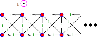
FIG. 1.: The basic cross linked lattice in a magnetic field. The numbers on the bonds represent phases giving half a unit of flux per plaquette. If we slightly slope the vertical bonds alternately in and out of the plane, the model is a chain of tetrahedra, linked on opposite edges.

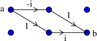
FIG. 2.: With half a unit of magnetic flux per plaquette, the paths for an electron to move two sites interfere destructively. A particle on site $a$ cannot reach $b$.

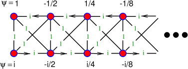
FIG. 3.: A zero energy state bound to the lattice end.

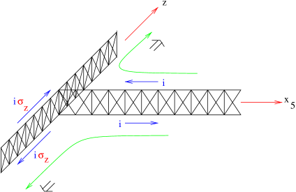
FIG. 4.: Joining a ladder onto the side of another. When the hopping on the main chain includes a spin matrix, this is a helicity filter. A particle traveling down the side chain turns towards the direction of its spin.

- [1] W. Shockley, Phys. Rev. 56, 317 (1939); F. Seitz, The Modern Theory of Solids, (McGraw-Hill, 1940), p. 323-4; W. G. Pollard, Phys. Rev. 56, 324 (1939).
- [2] B. I. Halperin, Phys. Rev. B 25, 2185 (1982); M. Stone, Phys. Rev. B42, 8399 (1995).
- [3] D. Kaplan, Phys. Lett. B288 (1992) 342; V. Furman and Y. Shamir, Nucl. Phys. B439, 54 (1995).
- [4] T. Blum and A. Soni, Phys. Rev. D56, 174 (1997); Phys. Rev. Lett. 79, 3595 (1997).
- [5] M. Creutz and I. Horvath, Phys. Rev. D50, 2297 (1994); Nucl. Phys. B34 (Proc. Suppl.), 586 (1994).
- [6] M. Creutz, Phys. Rev. D35, 1460 (1987).