UTCCP-P-61 Comparative Study of full QCD Hadron Spectrum and Static Quark Potential with Improved Actions

Abstract

We investigate effects of action improvement on the light hadron spectrum and the static quark potential in two-flavor QCD for $a^{-1}\approx 1$ GeV and $m_{\rm PS}/m_{\rm V}=0.7$–0.9. We compare a renormalization group improved action with the plaquette action for gluons, and the SW-clover action with the Wilson action for quarks. We find a significant improvement in the hadron spectrum by improving the quark action, while the gluon improvement is crucial for a rotationally invariant static potential. We also explore the region of light quark masses corresponding to $m_{\rm PS}/m_{\rm V}\geq 0.4$ on a 2.7 fm lattice using the improved gauge and quark action. A flattening of the potential is not observed up to 2 fm.

I Introduction

With the progress over the last few years of quenched simulations of QCD, it has become increasingly clear that the quenched hadron spectrum shows deviations from the experiment if examined at a precision better than 5–10%. For light hadrons the first indication was that the strange quark mass cannot be set consistently from pseudo scalar and vector meson channels in quenched QCD [1, 2, 3]. For heavy quark systems calculations both with relativistic [4] and non-relativistic [5] quark actions have shown that the fine structure of quarkonium spectra can not be reproduced on quenched gluon configurations. Most recently an extensive calculation by the CP-PACS collaboration found a systematic departure of both the light meson and baryon spectra from experiment [6]. These results raise the question as to whether the discrepancies can be accounted for by the inclusion of dynamical sea quarks. It is therefore timely to study more thoroughly the effects of full QCD in order to answer this question.

Full QCD simulations are, however, computationally much more expensive than those of quenched QCD. Simple scaling estimates coupled with past experience place a hundred-fold or more increase in the amount of computations for full QCD compared to that of quenched QCD with current algorithms. Since $32^{3}\!\times\!64$ is a typical maximal lattice size for quenched QCD which can be simulated with high statistics on computers with a speed in the 10 GFLOPS range [2, 7], reliable full QCD results are difficult to obtain on lattice sizes exceeding $32^{3}\!\times\!64$ even with TFLOPS-class computers such as CP-PACS [8] and QCDSP [9]. Recalling that a physical lattice size of $L\approx 2.5$–3.0 fm is needed to avoid finite-size effects [7, 10, 11], the smallest lattice spacing one can reasonably reach at present is therefore $a^{-1}\approx 2$ GeV. Hence lattice discretization errors have to be controlled through simulations carried out at inverse lattice spacings below this value, e.g. in the range $a^{-1}\approx 1-2$ GeV. It is, however, known that with the standard plaquette and Wilson quark actions discretization errors are already of order 10% even for $a^{-1}\approx 2$ GeV. These observations suggest the use of improved actions for simulations of full QCD.

Studies of improved actions have been widely pursued in the last few years. Detailed tests of improvement for the hadron spectrum, however, have been carried out mostly within quenched QCD [12, 13, 14, 15, 16, 17, 18, 19] with only a few full QCD attempts [20, 21, 22]. In particular, a systematic investigation of how gauge and quark action improvement, taken separately, affects light hadron observables has not been carried out in full QCD. Prior to embarking on a large scale simulation, we examine this question as the first subject of the full QCD program on the CP-PACS computer.

For a systematic comparison of action improvement we employ four possible types of action combinations, the standard plaquette or a renormalization-group improved action [23] for the gauge part, and the standard Wilson or the improvement of Sheikholeslami and Wohlert [24] for the quark part. Since effects of improvement are clearer to discern at coarser lattice spacings, we carry out simulations at an inverse lattice spacing of $a^{-1}\approx 1$ GeV with quark masses in the range corresponding to $m_{\rm PS}/m_{\rm V}\approx 0.7$–0.9. Results for the four action combinations are used for comparative tests of improvement on the light hadron spectrum and the static quark potential.

Another limiting factor for full QCD simulations is how close one can approach the chiral limit with present computing power. To investigate this question we take the action in which both gauge and quark parts are improved, and carry out simulations down to a quark mass corresponding to $m_{\rm PS}/m_{\rm V}\approx 0.4$. In addition to exploring the chiral behavior of hadron masses, this simulation allows an examination of signs of string breaking in the static quark-antiquark potential.

In this article we present results of our study on the two questions discussed above, expounding on the preliminary accounts reported in Refs. [25, 26]. We begin with discussions on our choice of actions for our comparative studies in Sec. II. Details of the full QCD configuration generation procedure and measurements of hadron masses and potential are described in Sec. III. Results for the hadron masses are discussed in Sec. IV where, after a description of the chiral extrapolation or interpolation of our data, we examine the effects of action improvement for the scaling behavior of hadron mass ratios. In Sec. V we turn to discuss the static potential. The influence of action improvement on the restoration of rotational symmetry of the potential is examined, and the consistency of the lattice spacing determined from the vector meson mass and the string tension is discussed. In Sec. VI we report on our effort to approach the chiral limit, where our attempt to observe a flattening of the potential at large distances due to string breaking is also presented. We end with a brief conclusion in Sec. VII. Detailed numerical results on run performances, hadron masses and string tensions are collected at the end in Appendices A, B and C.

II Choice of action

The discretization error of the standard plaquette gauge action is $O(a^{2})$ while that of the Wilson quark action is $O(a)$. In principle one would only need to improve the quark action to the same order as the gauge action. On the other hand, violations of rotational invariance have been found to be strong for the plaquette gauge action at coarse lattice spacings [27, 28]. Hence improving the gauge action is still advantageous for coarse lattices. In this spirit we employ (besides the standard actions) improved actions both in the gauge and quark sectors in the forms specified below.

Let us denote the standard plaquette gauge action by P. Improving this action requires the addition of Wilson loops with a perimeter of six links or more. The number, the precise form and the coefficients of the added terms differ depending on the principle one follows for the improvement [29]. In this study we test the action determined by an approximate block-spin renormalization group analysis of Wilson loops, denoted by R in the pursuant, which is given by [23]

$$S_{g}^{\rm\bf R}={\beta\over 6}\left(c_{0}\sum W_{1\times 1}+c_{1}\sum W_{1\times 2}\right),$$ (1)

where the $1\times 2$ rectangular shaped Wilson loop $W_{1\times 2}$ has the coefficient $c_{1}=-0.331$ and from the normalization condition defining the bare coupling $\beta=6/g_{0}^{2}$ follows $c_{0}=1-8c_{1}=3.648$.

The discretization error of the R action is still $O(a^{2})$. The coefficients of $O(a^{2})$ terms in physical quantities, however, are expected to be reduced from those of the plaquette action. Indeed, the quenched static quark potential calculated with this action was found to exhibit good rotational symmetry and scaling already at $a^{-1}\approx 1$ GeV [30], and so does the scaling of the ratio $T_{c}/\sqrt{\sigma}$ of the critical temperature of the pure gauge deconfining phase transition and the string tension $\sigma$ [30]. The degree of improvement is similar to those observed for tadpole-improved and fixed point actions [27, 28].

To improve the quark action we adopt the clover improvement proposed by Sheikholeslami and Wohlert [24], denoted by C in the following and defined by

$$D_{xy}^{\rm\bf C}=D_{xy}^{\rm\bf W}-\,\delta_{xy}c_{\rm SW}K\sum_{\mu<\nu}\sigma_{\mu\nu}F_{\mu\nu},$$ (2)

where $D_{xy}^{\rm\bf W}$ is the standard Wilson quark matrix given by

$$D_{xy}^{\rm\bf W}=\delta_{xy}-K\sum_{\mu}\{(1-\gamma_{\mu})U_{x,\mu}\delta_{x+\hat{\mu},y}+(1+\gamma_{\mu})U_{x,\mu}^{{\dagger}}\delta_{x,y+\hat{\mu}}\}$$ (3)

and $F_{\mu\nu}$ is the lattice discretization of the field strength,

$$F_{\mu\nu}=\frac{1}{8i}(f_{\mu\nu}-f_{\mu\nu}^{{\dagger}}),$$ (4)

where $f_{\mu\nu}$ is the standard clover-shaped combination of gauge links.

The complete removal of $O(a)$ errors requires a non-perturbative tuning of the clover coefficient $c_{\rm SW}$. This has been carried out for the plaquette gauge action in both quenched [31, 32] and two-flavor full QCD [33]. A similar analysis for the R gauge action is yet to be made, however. In this study we compare three different choices:

• The tree level value $c_{\rm SW}=1$.

• The mean-field (MF) improved value [34] $c_{\rm SW}=P^{-3/4}$ with $P$ the self-consistently determined plaquette average.

• A perturbative mean-field (pMF) improved value $c_{\rm SW}=P^{-3/4}$ with the plaquette $P$ calculated in one-loop perturbation theory. For the R gauge action $P=1-0.8412\cdot\beta^{-1}$ [23].

For all three choices the leading discretization error in physical quantities is $O(g_{0}^{2}a)$. The magnitude of the coefficients of this term should be reduced in the cases of (b) and (c) as compared to (a). The one-loop value of $c_{\rm SW}$ has been recently reported to be $c_{\rm SW}=1+0.678(18)/\beta$ [35]. This value is close to the pMF value $c_{\rm SW}^{\rm pMF}=1+0.631/\beta+\cdots$. We also find that the one-loop value of $P$ reproduces the measured values from simulations within 10% for the R action. Hence the pMF value of the clover coefficient is similar to the MF value employed in (b). The advantage of the pMF choice is that it does not require a self-consistent tuning of $c_{\rm SW}$ for each choice of $\beta$ and $K$.

We carry out simulations employing either the plaquette (P) or rectangular action (R) for gluons, combining it with either the Wilson (W) or clover action (C) for quarks.

III Simulations

A choice of simulation parameters

We choose the coupling constant $\beta$ so that it gives an inverse lattice spacing of $a^{-1}\approx 1$ GeV. For each action combination we choose at least two values of $\beta$ to allow us to interpolate (or extrapolate) to a desired common lattice spacing.

Simulations are generally carried out at three values of the hopping parameter $K$ corresponding to $m_{\rm PS}/m_{\rm V}\approx 0.7$–0.9. The lattice size employed is $12^{3}\!\times\!32$.

In Table I we give an overview of the calculations performed for the action comparison. Details of the simulation parameters at each run are collated in Appendix A. Our procedure for estimating the critical hopping parameter $K_{c}$, and the physical scale of lattice spacing either from the $\rho$ meson mass ($a_{\rho}$) or the string tension ($a_{\sigma}$) will be discussed in Sec. IV A and Sec. V C.

We take the RC_pMF action at $\beta=1.9$ to explore how close one can take the calculation towards the chiral limit. For this study we employ two lattice sizes $12^{3}\!\times\!32$ and $16^{3}\!\times\!32$. In Table II we list the main features of these two runs whereas details can be found in Appendix A.

B configuration generation and matrix inversion

Simulations are carried out for two flavors of dynamical quarks using the hybrid Monte Carlo (HMC) algorithm. The integration of molecular dynamics (MD) equations is made with the standard leapfrog scheme and with a step size $\Delta\tau$ chosen to yield an acceptance ratio of 70–90% for trajectories of unit length. The actual values chosen for $\Delta\tau$ in each case and the measured acceptance are given in Appendix A.

For the inversion of the fermion matrix we employed the minimal residue (MR) algorithm for our early simulations but switched later to BiCGStab[36]. In both cases we use an even-odd preconditioning of the quark matrix $D$. $D$ can be decomposed into

$$D(K)=M-K(D_{eo}+D_{oe}),$$ (5)

where $M$ is only defined on single sites and the remaining connects neighboring sites. For the Wilson quark action $M$ is a unit matrix, whereas for the clover action it is non-trivial in color and Dirac space. The even-odd preconditioning consists of solving the equation $AG_{e}=B_{e}^{\prime}$ where $A=1-K^{2}M_{e}^{-1}D_{eo}M_{o}^{-1}D_{oe}$ and $B_{e}^{\prime}=M_{e}^{-1}\left(B_{e}+KD_{eo}M_{o}^{-1}B_{o}\right)$ instead of the equation $D(K)G=B$. As an initial guess for the solution vector on even sites, the right-hand-side vector $G_{e}=B_{e}^{\prime}$ is used. The preconditioning requires the inversion of the local matrix $M$, which is trivial for the Wilson quark action. For the clover quark action we precalculate $M^{-1}$ and store it before the solver starts.

As a stopping condition for the matrix inversion during the fermionic force evaluation we generally use, on the $12^{3}\!\times\!32$ lattice, the criterion

$$r_{1}=||DG-B||^{2}\leq 10^{-10}$$ (6)

which we found to be approximately equivalent to the condition

$$r_{2}=||DG-B||/||G||\leq 10^{-8}.$$ (7)

The actual stopping conditions chosen for each run and the number of iterations needed to reach this condition are listed in Appendix A. For the evaluation of the Hamiltonian we choose stricter stopping criteria for $r_{1}$ between $10^{-14}$ and $10^{-18}$.

A necessary condition for the validity of the HMC algorithm is the reversibility of the MD evolution [37]. The CP-PACS computer, on which the present work is made, employs 64 bit arithmetic for floating point operations. Flipping the sign of momenta after a unit trajectory, with the stopping condition (7) above, we checked that, (i) the gauge link and conjugate momenta variables return to the starting values within a relative error of less than $10^{-7}$ on the average, and (ii) the relative error in the evaluation of the Hamiltonian is less than $10^{-10}$ (absolute error better than $10^{-4}$ for the $16^{3}\!\times\!32$ lattice where the check was made) so that the effects in the accept/reject procedure are far below the level of statistical fluctuations.

At each simulated parameter we first run for 100–200 HMC trajectories of unit length for thermalization and then generate 500–1500 trajectories for measurements. Hadron propagators are measured on configurations separated by 5 trajectories. The static quark potential is measured on a subset of the configurations separated by either 5 or 10 trajectories. The detailed numbers are again given in Appendix A.

C hadron mass measurement

We calculate quark propagators for the hopping parameter equal to that for the dynamical quarks used in the configuration generation. Two quark propagators are prepared for each configuration, one with the point source and the other with an exponentially smeared source with the smearing function $\psi(r)=A\exp(-Br)$. For the latter we fix the gauge configuration to the Coulomb gauge. The choice of the smearing parameters $A$ and $B$ is guided by previous quenched results for the pion wave function [38], readjusted by hand so that hadron effective masses reach a plateau as soon as possible.

Hadron propagators are constructed by combining quark propagators for the point (P) or the smeared (S) sources in various ways, but always adopting the point sink. For example, PS represents a meson propagator calculated with the point source for quark and the smeared source for antiquark. In Fig. 1 we show a typical example of effective masses for a variety of source combinations.

In most cases the effective masses for the SS (SSS for baryons) propagators comes from below, show the best plateau behavior, and have the smallest statistical errors estimated with the jackknife procedure. We therefore determine hadron masses with a fit to SS (SSS) hadron propagators, supplementing results for other source combinations as a guide in choosing the fit range.

Hadron masses are extracted from propagators by employing a single hyperbolic cosine fit for mesons and a single exponential fit for baryons. We use uncorrelated fits and determine the error with the jackknife method. While our runs of at most 1500 HMC trajectories are not really long enough to carry out detailed autocorrelation analysis, examining the bin size dependence of the estimated error indicates a bin size of 5 configurations or 25 HMC trajectories to be a reasonable choice, which we adopt for all of our error analyses.

The hadron mass results for all our runs are collected in Appendix B.

D potential measurement

We measure Wilson loops $W(r,t)$ both in the on- and off-axis directions in space. The spatial paths of $W(r,t)$ are formed by connecting one of the following spatial vectors repeatedly,

$$(1,0,0),\>(1,1,0),\>(2,1,0),\>(1,1,1),\>(2,1,1),\>(2,2,1).$$ (8)

We measure $W(r,t)$ up to $r\leq 6$ and $t\leq 8$ on the $12^{3}\!\times\!32$ lattice, while we enlarge the largest spatial size to $r\leq 4\sqrt{3}$ on the $16^{3}\!\times\!32$ lattice in order to investigate the large distance behavior of the potential. The smearing procedure of Ref. [39] is applied to the link variables, up to 6 times on the $12^{3}\!\times\!32$ lattice and up to 8 times on the $16^{3}\!\times\!32$ lattice, respectively. The Wilson loop is measured at every smearing step in order to choose the optimal smearing number for each value of $r$.

We extract the potential $V(r)$ and the overlap function $C(r)$ by a fully correlated fit of the Wilson loop to the form

$$W(r,t)=C(r)\ {\rm exp}\left[-V(r)t\right].$$ (9)

The optimum smearing number at each $r$ is determined by the condition that the overlap $C(r)$ takes the largest value smaller than 1.

Typical results for the effective mass defined by

$$m_{\rm eff}={\rm ln}\left[W(r,t)/W(r,t+1)\right],$$ (10)

are shown in Fig. 2. We find that noise generally dominates over the signal for $t>4$. Thus we set the upper limit of the fitting range to $t_{\rm max}=4$. Since choosing the lower limit $t_{\rm min}=1$ leads to an increase of ${\chi}^{2}/{\rm d.o.f}$ by 3–10 times compared to the choice $t_{\rm min}=2$ for most values of $r$ and simulation parameters, we fix the fitting range to be $t=2$–4.

The statistical error of $V(r)$ is estimated by the jackknife method. We find that a bin size of 30 HMC trajectories is generally sufficient to ensure stability of errors against bin size. We therefore adopt this bin size for all of our error estimates with potential data.

IV Hadron spectrum

A chiral fits

A basic parameter characterizing the chiral behavior of hadron masses is the critical hopping parameter $K_{c}$ at which the pseudo scalar meson mass $m_{\rm PS}a$ vanishes. Results for $(m_{\rm PS}a)^{2}$ exhibit deviations from a linear function in $1/K$, and hence we extract $K_{c}$ by assuming

$$(m_{\rm PS}a)^{2}=B_{\rm PS}\left(\frac{1}{K}-\frac{1}{K_{c}}\right)+C_{\rm PS}\left(\frac{1}{K}-\frac{1}{K_{c}}\right)^{2}.$$ (11)

The fitted values of the critical hopping parameter are listed in Table I and II.

Another important parameter is the vector meson mass $m_{\rm V}a$ in the chiral limit $m_{\rm PS}a=0$, which allows us to set the physical lattice spacing. We determine this quantity by a chiral fit of the vector meson mass in terms of the pseudo scalar meson mass, both of which are measured quantities. Our results for this relation show curvature (see Fig. 8 in Sec. VI A for an example), and hence for the fitting function we employ

$$m_{\rm V}a=A_{\rm V}+B_{\rm V}(m_{\rm PS}a)^{2}+C_{\rm V}(m_{\rm PS}a)^{3},$$ (12)

where the cubic term is inspired by chiral perturbation theory.

A practical problem with this fit is that we have only three data points for most of our runs. We estimate systematic uncertainties in the extrapolation by repeating the fit without the cubic term to the two points of data for lighter quark masses. Results for the vector meson mass in the chiral limit, translated into the lattice spacing through $a_{\rho}=A_{\rm V}/768{\rm MeV}$, are listed in Table I and II.

Results for the nucleon and $\Delta$ also show curvature in terms of $m_{\rm PS}a$. We therefore fit them employing a cubic polynomial without the linear term (12) as for the vector meson mass.

B scaling of mass ratios

We show in Fig. 3 a compilation of our hadron mass results for the four action combinations in terms of the mass ratios $m_{\rm N}/m_{\rm V}$ and $m_{\Delta}/m_{\rm V}$ as a function of $(m_{\rm PS}/m_{\rm V})^{2}$. In order to avoid overcluttering of points, we include results for only two values of $\beta$ per action combination. Furthermore, for the PC action combination the results with $c_{\rm SW}=$ MF are displayed whereas for the RC action results for $c_{\rm SW}=$ pMF are shown.

We observe two features in this figure. In the first instance, for each action combination the baryon to vector meson mass ratio decreases as the coupling decreases. This is a well-known trend of scaling violation for Wilson-type quark actions. Secondly, the magnitude of scaling violation, measured by the distance from the phenomenological curve (solid line in Fig. 3) [40] has an order where ${\sf\bf PW}>{\sf\bf RW}>{\sf\bf PC}>{\sf\bf RC}$. In particular the results for the PC and RC cases show a significant improvement over those for the PW and RW cases in that they lie close to the phenomenological curve even though the lattice spacing is as large as $a_{\rho}^{-1}\approx 1$–1.3 GeV (see Tables I and II).

A point of caution, however, is that the lattice spacings for the data sets displayed in Fig. 3 do not exactly coincide. In order to disentangle effects associated with action improvement from those of a finer lattice spacing for each action, we need to plot results at the same lattice spacing.

One way to make such a comparison is to take a cross section of Fig. 3 at a fixed value of $m_{\rm PS}/m_{\rm V}$ and plot the resulting value of $m_{\rm N,\Delta}/m_{\rm V}$ as a function of $m_{\rm V}a$ at that value of $m_{\rm PS}/m_{\rm V}$. This requires an interpolation of hadron mass results, for which we employ the cubic chiral fits described in Sec. IV A and the jackknife method for error estimation.

In Fig. 4 we show results of this analysis for $m_{\rm N}/m_{\rm V}$ and $m_{\Delta}/m_{\rm V}$ at $m_{\rm PS}/m_{\rm V}=0.8$. It is interesting to observe that the PW and RW results lie almost on a single curve, while the PC and RC results, respectively using the MF and pMF value of $c_{\rm SW}$, fall on a different, much flatter curve. This clearly shows that the improvement of the gauge action has little effect on decreasing the scaling violation in the baryon masses. The improvement is due to the use of the clover quark action for the PC and RC cases. An apparently better behavior of RW results in Fig. 3 compared to those for the PW case is merely an effect of the finer lattice spacing of the former.

We have commented in Sec. II that the values of $c_{\rm SW}$ for the MF and pMF cases are similar. This would explain why results for the PC action with the MF value of $c_{\rm SW}$ and those for the RC action with the pMF value of $c_{\rm SW}$ lie almost on a single curve. For both MF and pMF choices, the magnitude of $c_{\rm SW}$ is significantly larger than the tree-level value $c_{\rm SW}=1$. As is shown in Fig. 4 with open symbols, the degree of improvement with the tree-level $c_{\rm SW}$ is substantially less than those for the MF and pMF choices.

V Static quark potential

A restoration of rotational symmetry

In Fig. 5, we plot our potential data for the four action combinations at a quark mass corresponding to ${m_{\rm PS}}/{m_{\rm V}}\approx 0.8$ and $a^{-1}\approx 1$ GeV. We find a sizable violation of rotational symmetry in the PW case at this coarse lattice spacing. Looking at the potential for the PC case, we cannot observe any noticeable restoration of the symmetry. In contrast, a remarkable restoration of rotational symmetry is apparent in the RW and RC cases.

In order to quantify the violation of rotational symmetry and its improvement depending on the action choice, we consider the difference between the on-axis and off-axis potential at a distance $r=3$ defined by

$$\Delta V=\frac{V\left(r\!=\!\left(3,0,0\right)\right)-V\left(r\!=\!\left(2,2,1\right)\right)}{V\left(r\!=\!\left(3,0,0\right)\right)+V\left(r\!=\!\left(2,2,1\right)\right)}.$$ (13)

We find that the value of $\Delta V$ monotonously decreases as the sea quark mass decreases for most cases. We ascribe this trend to the fact that one effect of dynamical sea quarks is to renormalize the coupling toward a smaller value, and hence reduces violation of rotational symmetry.

In order to make a comparison at the same quark mass, we estimate $\Delta V$ at $m_{\rm PS}/m_{\rm V}=0.8$ by an interpolation as a linear function of $(m_{\rm PS}a)^{2}$. In Fig. 6 we plot results for $\Delta V$ obtained in this way against the value of $m_{\rm V}a$ at $m_{\rm PS}/m_{\rm V}=0.8$. This figure confirms the qualitative impression from Fig. 5. Rotational symmetry is badly violated for the PW and PC cases, which is significantly improved by changing the gauge action as demonstrated by the small values of $\Delta V$ for the RW and RC results. In contrast the effect of quark action improvement on the restoration of rotational symmetry appears to be small. This may not be surprising since dynamical quarks affect the static potential only indirectly through vacuum polarization effects.

B string tension

The static potential in full QCD is expected to flatten at large distances due to string breaking. None of our potential data, which typically extends up to the distance of $r\approx 1$ fm, show signs of such a behavior, but rather increase linearly. As we discuss in more detail in Sec. VI this is probably due to a poor overlap of the Wilson loop operator with the state of a broken string. This suggests that we can extract the string tension from the present data for the potential $V(r)$ by assuming the form

$$V(r)=V_{0}-\frac{\alpha}{r}+\sigma r.$$ (14)

In practice we find that the Coulomb coefficient $\alpha$ is difficult to determine from the fit, even if we introduce the tree-level correction term corresponding to the one lattice gluon exchange diagram. This may be due to the fact that our potential data taken at coarse lattice spacings do not have enough points at short distance to constrain the Coulomb term. As an alternative we test a two-parameter fitting with a fixed Coulomb term coefficient ${\alpha}_{\rm fixed}=0.1$, 0.125, …, 0.475, and 0.5, using the fitting range $r_{\rm min}$–$r_{\rm max}$ with $r_{\rm min}=1$, $\sqrt{2}$, $\sqrt{3}$ and $r_{\rm max}=5$–6. We find that the value of ${\chi}^{2}/{\rm d.o.f}$ takes its minimum value around ${\alpha}_{\rm fixed}=0.3$–$0.4$ for most fitting ranges and simulation parameters.

Based on this result, we extract the string tension by fitting the potential at large distances, where a linear behavior dominates, to the form (14) with a fixed Coulomb coefficient ${\alpha}_{\rm fixed}=0.35$. The shift of the fitted $\sigma$ over the range $\alpha=0.3$–$0.4$ is taken into estimates of the systematic error.

The result for the string tension $\sigma$ with this two-parameter fit is quite stable against variations of $r_{\rm max}$. It does depend more on $r_{\rm min}$, however. This leads us to repeat the two-parameter fit with ${\alpha}_{\rm fixed}=0.35$ over the interval of $r_{\rm min}$ listed in Appendix C, and determine the central value of $\sigma$ by the weighted average of the results over the ranges. The variance over the ranges are included into the systematic error of $\sigma$. We collate the final results for the string tension $\sigma$ in Appendix C.

C consistency in lattice spacings

The scaling violation in the ratio $m_{\rho}/\sqrt{\sigma}$ leads to an inconsistency in the lattice spacings determined from the $\rho$ meson mass $a_{\rho}$ and the string tension $a_{\sigma}$ in the chiral limit. Thus, examination of this consistency provides another test of effectiveness of improved actions. For the physical value we use $m_{\rho}=768$ MeV and $\sqrt{\sigma}=440$ MeV. We should note that the latter value is uncertain by about 5–10% since the string tension is not a directly measurable quantity by experiment.

The chiral extrapolation of the vector meson mass was already discussed in Sec. IV A. We follow a similar procedure for the chiral extrapolation of the string tension. Namely we fit results to a form

$${\sigma}a^{2}=A_{\sigma}+B_{\sigma}{\cdot}(m_{\rm PS}a)^{2}+C_{\sigma}{\cdot}(m_{\rm PS}a)^{3}.$$ (15)

In most cases we find a quadratic ansatz ($C_{\sigma}=0$) to be sufficient, which we then adopt for all data sets. Results for the string tension in the chiral limit, converted to the physical scale of lattice spacing $a_{\sigma}$, are listed in Table I and II.

In Fig. 7 we plot $m_{\rm V}a/768{\rm MeV}$ and $\sqrt{\sigma}a/440{\rm MeV}$ as a function of $(m_{\rm PS}a)^{2}$ for the four action combinations with a similar lattice spacing $a^{-1}_{\rho}\approx 1$–$1.3$ GeV determined from the vector meson mass. A distinctive difference between the results for the Wilson and the clover quark action is clear; while results for $m_{\rm V}$ and $\sqrt{\sigma}$ cross each other at heavy quark masses where $m_{\rm PS}/m_{\rm V}\approx 0.75$–$0.8$ for the PW and RW cases, leading to a mismatch of $a_{\rho}$ and $a_{\sigma}$ in the chiral limit, the two sets of physical scales converge well toward the chiral limit for the PC and RC cases.

We expect the large discrepancy for the Wilson quark action to disappear closer to the continuum limit. This is supported by the results obtained at $\beta=5.5$ with $a^{-1}\approx 2$ GeV in Ref.[41]. Our results show that the clover term helps to improve the consistency between $a_{\rho}$ and $a_{\sigma}$ already at $a^{-1}\approx 1$ GeV.

VI Approaching the chiral limit

The analyses presented so far show that the RC action has the best scaling behavior for hadron masses and static quark potential among the four action combinations we have examined. We then take this action and attempt to lower the quark mass as much as possible.

Two runs are made at $\beta=1.9$, one on a $12^{3}\!\times\!32$ lattice down to $m_{\rm PS}/m_{\rm V}\approx 0.5$, and the other on a $16^{3}\!\times\!32$ lattice down to $m_{\rm PS}/m_{\rm V}\approx 0.4$. We discuss results from these runs below.

A hadrons with small quark masses

In Fig. 8 we plot the results of hadron masses as functions of $(m_{\rm PS}a)^{2}$. The existence of a curvature is observed, necessitating a cubic ansatz for extrapolation to the chiral limit. The lattice spacing determined from $m_{\rho}=768$ MeV equals $a_{\rho}=0.20(2)$ fm using mass results from the larger lattice. Hence the spatial size equals 2.4 fm ($12^{3}\!\times\!32$) and 3.2 fm ($16^{3}\!\times\!32$) for the two lattice sizes employed.

Finite-size effects are an important issue for precision determinations of the hadron mass spectrum. Our results in Fig. 8 do not show clear signs of such effects down to the second lightest mass, which corresponds to $m_{\rm PS}/m_{\rm V}\approx 0.5$. We feel, however, that it is premature to draw conclusions with the present low statistics of approximately 1000 trajectories.

The results for mass ratios are plotted in Fig. 9. While errors are large, and may even be underestimated because of the shortness of the runs, we find it encouraging that the ratios exhibit a trend of following the phenomenological curve toward the experimental points as the quark mass decreases. If we use the chiral extrapolation described above for the results on the $16^{3}\!\times\!32$ lattice, we obtain $m_{\rm N}/m_{\rm V}=1.342(25)$ and $m_{\rm\Delta}/m_{\rm V}=1.700(33)$ at the physical ratio $m_{\rm PS}/m_{\rm V}=0.1757$, which are less than 10% off the experimentally observed ratios of 1.223 and 1.603, respectively, despite the coarse lattice spacing of $a\approx 0.2$ fm.

B static potential at large distances

We have mentioned in Sec. V that our results for the static potential do not show signs of flattening, indicative of string breaking up to the distance of $r\approx 1$ fm. Similar results have been reported by other groups [42]. A possible reason for these results is that potential data do not extend to large enough distances where string breaking becomes energetically favorable. Another related possibility is that the dynamical quark masses, which in most cases correspond to $m_{\rm PS}/m_{\rm V}=0.7$–$0.9$, are too heavy. With our runs on the $16^{3}\!\times\!32$ lattice we can examine these points up to the distance of $r\approx 2$ fm and for quark masses down to $m_{\rm PS}/m_{\rm V}\approx 0.4$.

In Fig. 10 we plot our potential data obtained on the $16^{3}\!\times\!32$ lattice at the lightest sea quark mass corresponding to $m_{\rm PS}/m_{\rm V}\approx 0.4$. We find that the potential increases linearly up to $r\approx 2$ fm, without any clear signal of flattening. The situation is similar for our data at heavier sea quark masses.

An interesting and crucial question here is whether the Wilson loop operator has sufficient overlap with the ground state at large $r$ so that the potential in that state is reliably measured there [43]. In Fig. 11 we compare results for the overlap function $C(r)$ for the full QCD run at $m_{\rm PS}/m_{\rm V}\approx 0.4$ with that obtained in a quenched run with the R gauge action on a $9^{3}\!\times\!18$ lattice at $\beta=2.1508$ ($a^{-1}\approx 1$ GeV) [30]. For the quenched run the overlap $C(r)$ of the smeared Wilson loop operator with the ground string state is effectively 100 % at all distances. For full QCD, on the other hand, $C(r)$ significantly decreases as $r$ increases. Such a behavior of $C(r)$ is observed in all of our data including those taken with action choices other than RC. These results may be taken as a tantalizing hint that the Wilson loop operator develops mixings with states other than a single string, possibly a pair of static-light mesons in full QCD. We leave further investigations of this interesting question for future studies.

C computer time

An important practical information in full QCD is the computer time needed for the approach to the chiral limit. In Table III we assemble the relevant numbers for our runs on the $16^{3}\!\times\!32$ lattice. These runs have been performed on a partition of 256 nodes, which is 1/8 of the CP-PACS computer. For a partition of this size, our full QCD program, written in FORTRAN with the matrix multiplication in the quark solver hand-optimized in the assembly language, sustains about 37% of the peak speed of 75 GFLOPS. Adding the CPU time per trajectory of Table III, we find that accumulating 5000 trajectories for each of the 6 hopping parameters for this lattice size would take about 160 days with the full use of the CP-PACS computer. Carrying out such a simulation is certainly feasible. For larger lattice sizes such as $24^{3}\!\times\!48$, however, we would have to stop at $m_{\rm PS}/m_{\rm V}\approx 0.5$ since the run at $m_{\rm PS}/m_{\rm V}\approx 0.4$ alone increases the computer time by a factor two. Let us add that the CPU time for a unit of HMC trajectory increases roughly proportional to $(1/K-1/K_{c})^{-1.6}$ for the 4 smallest quark masses.

VII Conclusions

In this paper we have presented a detailed investigation of the effect of improving the gauge and the quark action in full QCD. We have found that the consequence of improving either of the actions is different depending on the observable examined.

For the light hadron spectrum the clover quark action with a mean-field improved coefficient drastically improves the scaling of hadron mass ratios. Improving the gauge action, on the other hand, has almost no influence in this aspect. The SW-clover action also has the good property that the physical scale determined from the vector meson mass and the string tension in the chiral limit of the sea quark are consistent already at scales $a^{-1}\approx 1$ GeV, which is not the case with the Wilson quark action.

We have also confirmed that the use of improved gauge actions leads to a significant decrease of the breaking of rotational symmetry of the static quark potential.

Finally, we have made an exploratory simulation toward the chiral limit employing a renormalization group improved gauge and clover improved quark actions.

The results obtained in the present study suggest that a significant step toward a systematic full QCD simulation can be made with the present computing power using improved gauge and quark actions at relatively coarse lattice spacings of $a^{-1}\approx 1$–2 GeV.

TABLE I.: Overview of the simulations on the $12^{3}\!\times\!32$ lattice for the action comparison.

action	$\beta$	$c_{\rm SW}$	$m_{\rm PS}/m_{\rm V}$	$K_{c}$	${a_{\rho}}$ [fm]	${a_{\sigma}}$ [fm]
PW	4.8	–	0.83,0.77,0.70	0.19286(14)	0.197(2)	–
PW	5.0	–	0.85,0.79,0.71	0.18291(7)	0.174${}^{+8}_{-22}$	0.2501(62)
RW	1.9	–	0.90,0.80,0.69	0.17398(7)	0.162${}^{+11}_{-15}$	–
RW	2.0	–	0.90,0.83,0.74	0.16726(8)	0.144${}^{+7}_{-13}$	0.1747(27)
PCtree	5.0	1.0	0.83,0.79,0.71	0.16631(18)	0.2157(4)	–
PCMF	5.0	1.805–1.855	0.81,0.76,0.71	0.14927(28)	0.238(1)	0.241(12)
PCMF	5.2	1.64–1.69	0.84,0.79,0.72	0.14298(6)	0.141${}^{+15}_{-24}$	0.1370(83)
PCMF	5.25	1.61–1.637	0.84,0.76	0.14252(4)	0.133(3)	0.1161(89)
RCpMF	1.9	1.55	0.85,0.78,0.69	0.14446(6)	0.199${}^{+14}_{-27}$	0.2050(40)
RCtree	2.0	1.0	0.88,0.83,0.71	0.15045(10)	0.160${}^{+10}_{-18}$	0.1638(42)
RCMF	2.0	1.515–1.54	0.90,0.86,0.79,0.70	0.14083(4)	0.146(3)	0.152(3)
RCpMF	2.0	1.505	0.91,0.79,0.71	0.14058(7)	0.146${}^{+35}_{-22}$	–

TABLE II.: Overview of the simulations exploring the chiral limit of full QCD.

size	$\beta$	$c_{\rm SW}$	$m_{\rm PS}/m_{\rm V}$	$K_{c}$	${a_{\rho}}$ [fm]	${a_{\sigma}}$ [fm]
$12^{3}\!\times\!32$	1.9	1.55	0.85,0.78,0.69,0.60,0.54	0.144432(18)	0.171(3)	–
$16^{3}\!\times\!32$	1.9	1.55	0.84,0.78,0.69,0.61,0.54,0.41	0.144434(10)	0.166(2)	0.1817(28)

TABLE III.: CPU time per HMC trajectory for the run at $\beta=1.9$ on the $16^{3}\!\times\!32$ lattice carried out on CP-PACS with 256 nodes (75 GFLOPS peak).

$K$	$(1/K-1/K_{c})/2$	$m_{\rm PS}/m_{\rm V}$	$\Delta\tau$	accept.	stop	$N_{\rm inv}$	CPU-time
0.1370	0.1879(2)	0.8446(15)	0.0075	0.86	$10^{-11}$	30	6.4 min.
0.1400	0.1096(2)	0.7793(19)	0.0075	0.80	$10^{-11}$	46	8.2 min.
0.1420	0.0593(2)	0.6899(33)	0.00625	0.77	$10^{-11}$	74	14.2 min.
0.1430	0.0347(2)	0.6110(44)	0.004	0.77	$10^{-11}$	116	32.3 min.
0.1435	0.0225(2)	0.5445(50)	0.0025	0.81	$10^{-12}$	181	77.6 min.
0.1440	0.0104(2)	0.4115(96)	0.0015	0.66	$10^{-12}$	344	230.4 min.

A Run Parameters

In this appendix we assemble information about our runs. An overview of the runs has been given in Table I. For the inversion of the quark matrix either the MR algorithm (M) or the BiCGStab algorithm (B) is used with the stopping condition $r_{1}\leq$ stop defined through Eq.(6). During the HMC update $D^{\dagger}D$ has to be inverted. We do this in two steps, first inverting $D^{\dagger}$ and then $D$. In the tables we quote the number of iterations $N_{\rm inv}$ needed for the first inversion $D^{\dagger}$. Finally we also quote the statistics, giving the number of configurations for spectrum and potential measurements separately. Configurations for the hadron spectrum are separated by 5 HMC trajectories, whereas for the potential the separation is either 5 or 10 trajectories. Unless stated otherwise the lattice size is $12^{3}\!\times\!32$.

TABLE IV.: Simulation parameters for the PW and RW action combination.

action	$\beta$	$K$	$\Delta\tau$	accept.	inverter	stop	$N_{\rm inv}$	#conf	#conf$\times$sep
								spect.	pot.
PW	4.8	0.1846	0.01	0.78	M	$10^{-10}$	100	222	–
		0.1874	0.005	0.88	M	$10^{-10}$	150	200	–
		0.1891	0.005	0.83	M	$10^{-10}$	199	200	–
	5.0	0.1779	0.01	0.79	M	$10^{-10}$	101	300	$89\times 5$
		0.1798	0.005	0.94	M	$10^{-10}$	147	301	$100\times 5$
		0.1811	0.005	0.88	M	$10^{-10}$	212	301	$100\times 5$
RW	1.9	0.1632	0.0125	0.82	M	$10^{-10}$	73	200	–
		0.1688	0.01	0.78	M	$10^{-10}$	136	200	$100\times 5$
		0.1713	0.008	0.71	M	$10^{-10}$	234	200	–
	2.0	0.1583	0.0125	0.79	M	$10^{-10}$	77	300	$100\times 5$
		0.1623	0.01	0.84	M	$10^{-10}$	128	300	$100\times 5$
		0.1644	0.008	0.82	M	$10^{-10}$	212	305	$96\times 5$

TABLE V.: Simulation parameters for the PC action combination.

$\beta$	$K$	$c_{\rm SW}$	$\Delta\tau$	accept.	inverter	stop	$N_{\rm inv}$	#conf	#conf$\times$sep
								spect.	pot.
5.0	0.1590	1.0	0.01	0.82	B	$10^{-10}$	37	100	–
	0.1610	1.0	0.008	0.83	B	$10^{-10}$	44	100	–
	0.1630	1.0	0.00625	0.80	B	$10^{-10}$	67	101	–
5.0	0.1415	1.855	0.01	0.73	B	$10^{-10}$	30	200	$100\times 10$
	0.1441	1.825	0.008	0.75	B	$10^{-10}$	42	200	$100\times 10$
	0.1455	1.805	0.00625	0.77	B	$10^{-10}$	55	200	$100\times 10$
5.2	0.1390	1.69	0.01	0.81	M	$10^{-10}$	72	248	$104\times 5$
	0.1410	1.655	0.008	0.83	M	$10^{-10}$	117	232	$100\times 5$
	0.1420	1.64	0.008	0.73	M	$10^{-10}$	203	200	$100\times 5$
5.25	0.1390	1.637	0.008	0.88	M	$10^{-10}$	88	198	$69\times 5$
	0.1410	1.61	0.00667	0.84	M	$10^{-10}$	183	194	$101\times 5$

TABLE VI.: Simulation parameters for the RC action combination. The run marked with (*) is on the $16^{3}\!\times\!32$ lattice.

$\beta$	$K$	$c_{\rm SW}$	$\Delta\tau$	accept.	inv.	stop	$N_{\rm inv}$	#conf	#conf$\times$sep
								spect.	pot.
$1.9^{*}$	0.1370	1.55	0.0075	0.86	B	$10^{-11}$	30	203	–
	0.1400	1.55	0.0075	0.80	B	$10^{-11}$	46	198	–
	0.1420	1.55	0.00625	0.77	B	$10^{-11}$	74	202	$92\times 10$
	0.1430	1.55	0.004	0.77	B	$10^{-11}$	116	212	$102\times 10$
	0.1435	1.55	0.0025	0.81	B	$10^{-12}$	181	263	–
	0.1440	1.55	0.0015	0.66	B	$10^{-12}$	344	79	$79\times 10$
1.9	0.1370	1.55	0.01	0.82	B	$10^{-10}$	28	267	$127\times 10$
	0.1400	1.55	0.01	0.78	B	$10^{-10}$	41	214	$104\times 10$
	0.1420	1.55	0.008	0.72	B	$10^{-10}$	66	324	$148\times 10$
	0.1430	1.55	0.005	0.77	B	$10^{-10}$	102	302	–
	0.1435	1.55	0.00333	0.79	B	$10^{-11}$	159	170	–
2.0	0.1420	1.0	0.01	0.87	B	$10^{-10}$	29	100	$50\times 10$
	0.1450	1.0	0.008	0.91	B	$10^{-10}$	42	100	$50\times 10$
	0.1480	1.0	0.00625	0.86	B	$10^{-10}$	81	100	$50\times 10$
2.0	0.1300	1.505	0.01	0.90	B	$10^{-10}$	21	100	–
	0.1370	1.505	0.008	0.86	B	$10^{-10}$	47	90	–
	0.1388	1.505	0.008	0.78	B	$10^{-10}$	79	90	–
2.0	0.1300	1.54	0.008	0.93	M	$10^{-10}$	42	201	$100\times 5$
	0.1340	1.529	0.008	0.90	M	$10^{-10}$	62	200	$100\times 10$
	0.1370	1.52	0.008	0.87	M/B	$10^{-10}$	102/50	200	$102\times 5$
	0.1388	1.515	0.00625	0.84	M/B	$10^{-10}$	181/84	200	$105\times 5$

B Hadron Masses

In this appendix we assemble the results of our hadron mass measurements. We quote numbers for pseudo scalar and vector mesons, nucleons and $\Delta$ baryons together with mass ratios against vector mesons. Additionally we quote numbers for the bare quark mass based on the axial Ward identity defined by

$$m_{q}a=-m_{\rm PS}a\lim_{t\rightarrow\infty}\frac{\sum_{\vec{x}}\langle A_{4}(\vec{x},t)P\rangle}{\sum_{\vec{x}}\langle P(\vec{x},t)P\rangle},$$ (B1)

where $A_{4}$ is the local axial current and $P$ is the pseudo scalar density. Masses are extracted with an uncorrelated fit to the propagator and the errors are determined with the jackknife method with bin size 5.

TABLE VII.: PW action combination: AWI quark mass and meson masses.

$\beta$	$K$	$m_{q}a$	$m_{\rm PS}a$	$m_{\rm V}a$	$m_{\rm PS}/m_{\rm V}$
4.8	0.1846	0.13400(68)	0.9350(9)	1.1276(18)	0.8291(12)
	0.1874	0.09269(80)	0.7918(13)	1.0263(25)	0.7715(17)
	0.1891	0.06523(70)	0.6716(16)	0.9559(45)	0.7026(32)
5.0	0.1779	0.13464(91)	0.9182(10)	1.0859(17)	0.8456(12)
	0.1798	0.09652(88)	0.7829(14)	0.9863(23)	0.7938(18)
	0.1811	0.0610(12)	0.6254(32)	0.8753(38)	0.7145(42)

TABLE VIII.: RW action combination: AWI quark mass and meson masses.

$\beta$	$K$	$m_{q}a$	$m_{\rm PS}a$	$m_{\rm V}a$	$m_{\rm PS}/m_{\rm V}$
1.9	0.1632	0.1972(15)	1.0557(11)	1.1743(16)	0.8990(9)
	0.1688	0.0977(13)	0.7525(19)	0.9377(35)	0.8025(26)
	0.1713	0.05281(84)	0.5469(21)	0.7935(52)	0.6892(43)
2.0	0.1583	0.1761(11)	0.9551(12)	1.0631(17)	0.8984(90)
	0.1623	0.10021(88)	0.7177(14)	0.8671(27)	0.8277(20)
	0.1644	0.06010(61)	0.5475(16)	0.7406(27)	0.7394(26)

TABLE IX.: PC action combination: AWI quark mass and meson masses.

$\beta$	$K$	$m_{q}a$	$m_{\rm PS}a$	$m_{\rm V}a$	$m_{\rm PS}/m_{\rm V}$
$5.0_{\rm tree}$	0.1590	0.2029(17)	1.1105(10)	1.3452(36)	0.8256(21)
	0.1610	0.1509(17)	0.9641(28)	1.2193(69)	0.7907(38)
	0.1630	0.0956(20)	0.7740(22)	1.0865(81)	0.7124(60)
$5.0_{\rm MF}$	0.1415	0.2211(17)	1.1970(18)	1.4769(44)	0.8104(26)
	0.1441	0.1574(15)	0.9961(19)	1.3156(65)	0.7571(36)
	0.1455	0.1176(15)	0.8588(42)	1.2024(99)	0.7143(44)
$5.2$	0.1390	0.1855(24)	1.0161(27)	1.2100(48)	0.8398(20)
	0.1410	0.1160(17)	0.7662(43)	0.9654(72)	0.7937(30)
	0.1420	0.0646(24)	0.5553(55)	0.7674(93)	0.7236(76)
$5.25$	0.1390	0.1435(19)	0.8479(30)	1.0155(42)	0.8350(26)
	0.1410	0.0731(17)	0.5532(42)	0.7296(91)	0.7581(57)

TABLE X.: RC action combination: AWI quark mass and meson masses. The run marked with (*) is on the $16^{3}\!\times\!32$ lattice.

$\beta$	$K$	$m_{q}a$	$m_{\rm PS}a$	$m_{\rm V}a$	$m_{\rm PS}/m_{\rm V}$
$1.9^{*}$	0.1370	0.2428(10)	1.1926(11)	1.4121(31)	0.8446(15)
	0.1400	0.1517(10)	0.9321(11)	1.1961(36)	0.7793(19)
	0.1420	0.08834(88)	0.6992(19)	1.0134(60)	0.6899(33)
	0.1430	0.05530(62)	0.5414(18)	0.8861(71)	0.6110(44)
	0.1435	0.03484(75)	0.4338(20)	0.7967(68)	0.5445(50)
	0.1440	0.0156(15)	0.2906(41)	0.706(15)	0.4115(96)
1.9	0.1370	0.2440(13)	1.1918(12)	1.4091(28)	0.8458(17)
	0.1400	0.1547(10)	0.9334(17)	1.2033(39)	0.7757(18)
	0.1420	0.08975(96)	0.6983(18)	1.0149(45)	0.6880(31)
	0.1430	0.05278(77)	0.5337(24)	0.8902(53)	0.5995(38)
	0.1435	0.0374(17)	0.4368(30)	0.802(10)	0.5448(82)
$2.0_{\rm tree}$	0.1420	0.2303(14)	1.0888(22)	1.2403(33)	0.8779(15)
	0.1450	0.1519(13)	0.8645(28)	1.0415(44)	0.8300(21)
	0.1480	0.0713(16)	0.5730(24)	0.8064(79)	0.7105(59)
$2.0_{\rm pMF}$	0.1300	0.3313(18)	1.3358(21)	1.4682(33)	0.9098(11)
	0.1370	0.1305(10)	0.7784(25)	0.9801(47)	0.7942(31)
	0.1388	0.0665(13)	0.5489(38)	0.773(11)	0.7098(77)
$2.0_{\rm MF}$	0.1300	0.3158(10)	1.2971(11)	1.4377(22)	0.9022(11)
	0.1340	0.2079(10)	1.0137(17)	1.1759(27)	0.8620(16)
	0.1370	0.1190(10)	0.7435(17)	0.9400(44)	0.7910(32)
	0.1388	0.0671(10)	0.5416(24)	0.7741(71)	0.6997(56)

TABLE XI.: PW action combination: baryon masses.

$\beta$	$K$	$m_{\rm N}a$	$m_{\Delta}a$	$m_{\rm N}/m_{\rm V}$	$m_{\Delta}/m_{\rm V}$
4.8	0.1846	2.009(12)	2.074(15)	1.782(11)	1.839(13)
	0.1874	1.817(18)	1.912(23)	1.771(18)	1.863(23)
	0.1891	1.647(20)	1.848(32)	1.723(22)	1.933(36)
5.0	0.1779	1.894(12)	1.976(17)	1.744(11)	1.819(16)
	0.1798	1.668(15)	1.775(13)	1.691(14)	1.799(12)
	0.1811	1.437(17)	1.559(18)	1.642(20)	1.781(19)

TABLE XII.: RW action combination: baryon masses.

$\beta$	$K$	$m_{\rm N}a$	$m_{\Delta}a$	$m_{\rm N}/m_{\rm V}$	$m_{\Delta}/m_{\rm V}$
1.9	0.1632	1.997(14)	2.044(15)	1.700(12)	1.740(13)
	0.1688	1.548(15)	1.650(21)	1.651(13)	1.760(20)
	0.1713	1.2643(88)	1.417(17)	1.593(12)	1.786(19)
2.0	0.1583	1.7589(57)	1.8150(77)	1.6545(48)	1.7073(62)
	0.1623	1.4214(77)	1.5008(90)	1.6392(80)	1.7308(84)
	0.1644	1.1752(80)	1.281(11)	1.587(10)	1.729(14)

TABLE XIII.: PC action combination: baryon masses.

$\beta$	$K$	$m_{\rm N}a$	$m_{\Delta}a$	$m_{\rm N}/m_{\rm V}$	$m_{\Delta}/m_{\rm V}$
$5.0_{\rm tree}$	0.1590	2.203(25)	2.358(30)	1.638(20)	1.753(23)
	0.1610	1.982(24)	2.110(30)	1.625(13)	1.730(18)
	0.1630	1.748(22)	1.868(44)	1.609(21)	1.719(40)
$5.0_{\rm MF}$	0.1415	2.343(24)	2.501(28)	1.586(16)	1.693(17)
	0.1441	2.041(20)	2.243(27)	1.551(14)	1.705(18)
	0.1455	1.851(21)	1.994(31)	1.539(15)	1.659(24)
5.2	0.1390	1.864(13)	1.980(16)	1.5408(88)	1.637(10)
	0.1410	1.481(12)	1.582(17)	1.5341(95)	1.639(12)
	0.1420	1.163(17)	1.241(21)	1.515(16)	1.617(16)
5.25	0.1390	1.5509(98)	1.638(14)	1.5273(65)	1.6134(93)
	0.1410	1.111(13)	1.212(19)	1.5221(97)	1.661(17)

TABLE XIV.: RC action combination: baryon masses. The run marked with (*) is on the $16^{3}\!\times\!32$ lattice.

$\beta$	$K$	$m_{\rm N}a$	$m_{\Delta}a$	$m_{\rm N}/m_{\rm V}$	$m_{\Delta}/m_{\rm V}$
$1.9^{*}$	0.1370	2.195(10)	2.296(15)	1.5547(66)	1.6263(97)
	0.1400	1.845(10)	1.978(13)	1.5428(64)	1.6541(92)
	0.1420	1.494(12)	1.662(17)	1.474(11)	1.640(17)
	0.1430	1.283(13)	1.501(17)	1.448(15)	1.694(19)
	0.1435	1.154(12)	1.368(24)	1.448(19)	1.717(28)
	0.1440	0.972(25)	1.171(32)	1.376(29)	1.658(33)
1.9	0.1370	2.2172(91)	2.358(20)	1.5735(61)	1.673(14)
	0.1400	1.8573(95)	2.009(12)	1.5434(77)	1.670(11)
	0.1420	1.5195(78)	1.712(11)	1.4972(76)	1.687(11)
	0.1430	1.274(11)	1.486(13)	1.431(13)	1.669(14)
	0.1435	1.173(22)	1.406(39)	1.463(28)	1.754(43)
$2.0_{\rm tree}$	0.1420	1.9605(86)	2.0646(90)	1.5807(67)	1.6647(60)
	0.1450	1.6293(87)	1.733(13)	1.5644(60)	1.6644(91)
	0.1480	1.197(15)	1.382(25)	1.485(18)	1.714(28)
$2.0_{\rm pMF}$	0.1300	2.286(10)	2.353(12)	1.5569(48)	1.6029(61)
	0.1370	1.4918(78)	1.622(14)	1.5220(77)	1.655(10)
	0.1388	1.150(16)	1.302(26)	1.487(22)	1.684(32)
$2.0_{\rm MF}$	0.1300	2.2242(46)	2.3057(61)	1.5471(27)	1.6038(37)
	0.1340	1.8185(53)	1.929(12)	1.5465(42)	1.6405(92)
	0.1370	1.419(10)	1.521(15)	1.5096(95)	1.618(13)
	0.1388	1.153(12)	1.308(19)	1.489(15)	1.689(20)

C String Tension

TABLE XV.: Results of string tension $\sigma$ in lattice units. The quoted error of $\sigma$ includes the estimate of the systematic error described in Sec.V B. We also show the fitting range $r_{\rm min}$–$r_{\rm max}$. The run marked with (*) is on the $16^{3}\!\times\!32$ lattice.

action	$\beta$	K	$\sigma$	$r_{\rm min}$	$r_{\rm max}$
PW	5.0	0.1779	0.324(38)	$2\sqrt{2}$–$2\sqrt{3}$	5
		0.1798	0.307(27)	$2\sqrt{2}$–$2\sqrt{3}$	5
		0.1811	0.335(11)	$2\sqrt{2}$–$2\sqrt{3}$	5
RW	1.9	0.1688	0.2980(53)	$2\sqrt{2}$–$2\sqrt{3}$	6
	2.0	0.1583	0.2678(60)	$2\sqrt{2}$–$2\sqrt{3}$	6
		0.1623	0.2143(42)	$2\sqrt{2}$–$2\sqrt{3}$	6
		0.1644	0.1864(42))	$2\sqrt{2}$–$2\sqrt{3}$	6
PCMF	5.0	0.1415	0.338(54)	$\sqrt{6}$–3	5
		0.1441	0.317(35)	$\sqrt{6}$–3	5
		0.1455	0.323(37)	$\sqrt{6}$–3	5
	5.2	0.1390	0.2192(90)	$2\sqrt{2}$–$2\sqrt{3}$	6
		0.1410	0.1588(50)	$2\sqrt{2}$–$2\sqrt{3}$	6
		0.1420	0.1255(39)	$2\sqrt{2}$–$2\sqrt{3}$	6
	5.25	0.1390	0.1453(59)	$2\sqrt{2}$–$2\sqrt{3}$	6
		0.1410	0.0969(34)	$2\sqrt{2}$–$2\sqrt{3}$	6
RCpMF	1.9	0.1370	0.3243(87)	$2\sqrt{2}$–3	5
		0.1400	0.2750(75)	$2\sqrt{2}$–3	5
		0.1420	0.2465(46)	$2\sqrt{2}$–3	5
RCpMF	$1.9^{*}$	0.1420	0.2375(60)	$2\sqrt{2}$–$2\sqrt{3}$	8
		0.1430	0.2094(51)	$2\sqrt{2}$–$2\sqrt{3}$	8
		0.1440	0.1755(57)	$2\sqrt{2}$–$2\sqrt{3}$	$3\sqrt{5}$
RCtree	2.0	0.1420	0.2583(81)	$2\sqrt{2}$–$2\sqrt{3}$	6
		0.1450	0.2097(47)	$2\sqrt{2}$–$2\sqrt{3}$	6
		0.1480	0.1642(53)	$2\sqrt{2}$–$2\sqrt{3}$	6
RCMF	2.0	0.1300	0.2147(57)	$2\sqrt{2}$–$2\sqrt{3}$	6
		0.1340	0.1832(48)	$2\sqrt{2}$–$2\sqrt{3}$	6
		0.1370	0.1506(38)	$2\sqrt{2}$–$2\sqrt{3}$	6
		0.1370	0.1251(35)	$2\sqrt{2}$–$2\sqrt{3}$	6

FIG. 1.: Example of effective mass plots for pseudo scalar, vector, nucleon and $\Delta$ on a $12^{3}\!\times\!32$ lattice. Circles are effective masses where all quark propagators have point sources (PP or PPP). For squares all quark propagators have smeared sources (SS or SSS) and triangles are for mixed combinations of sources (PS, PPS or PSS). Solid lines denote the results from mass fits to SS or SSS correlators. Dashed lines show the one standard deviation error band determined by jackknife analysis.

FIG. 2.: Effective masses of the static quark potential for the optimum smearing at $r=3a$ for four action combinations.

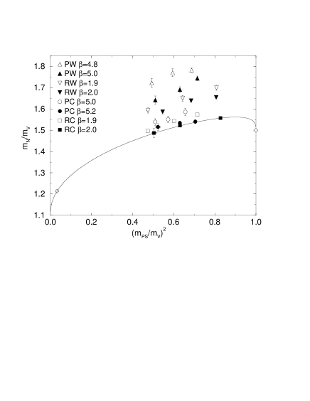
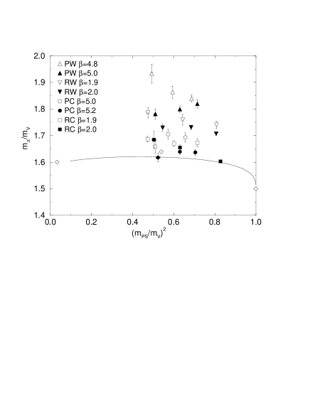
FIG. 3.: $m_{\rm N}/m_{\rm V}$ and $m_{\Delta}/m_{\rm V}$ as function of $(m_{\rm PS}/m_{\rm V})^{2}$ for four combinations of the action. Diamonds are experimental points corresponding to ${\rm N}(940)/\rho(770)$, $\Delta(1232)/\rho(770)$ and $\Omega(1672)/\phi(1020)$.

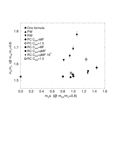
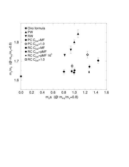
FIG. 4.: Scaling behavior of $m_{\rm N}/m_{\rm V}$ and $m_{\Delta}/m_{\rm V}$ at fixed $m_{\rm PS}/m_{\rm V}=0.8$ as function of $m_{\rm V}a$.

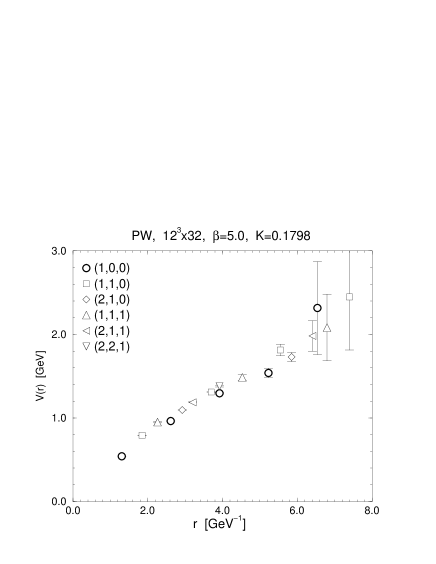
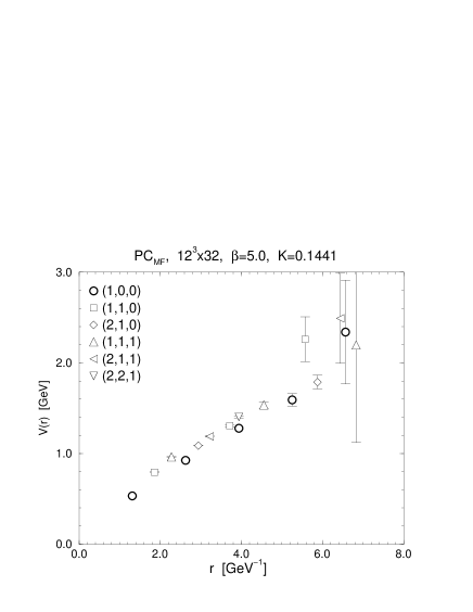
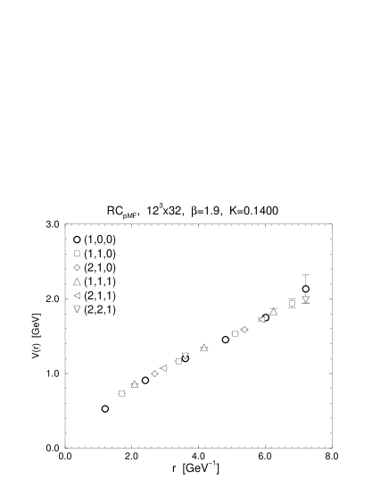
FIG. 5.: Static quark potential for the four action combinations at $m_{\rm PS}/m_{\rm V}\simeq 0.8$ on the $12^{3}\!\times\!32$ lattice with a lattice spacing $a\approx 1{\rm GeV^{-1}}$. Scales are set by the lattice spacing determined from the string tension. Different symbols correspond to the potential data measured in different spatial directions along the vector indicated in the figure.

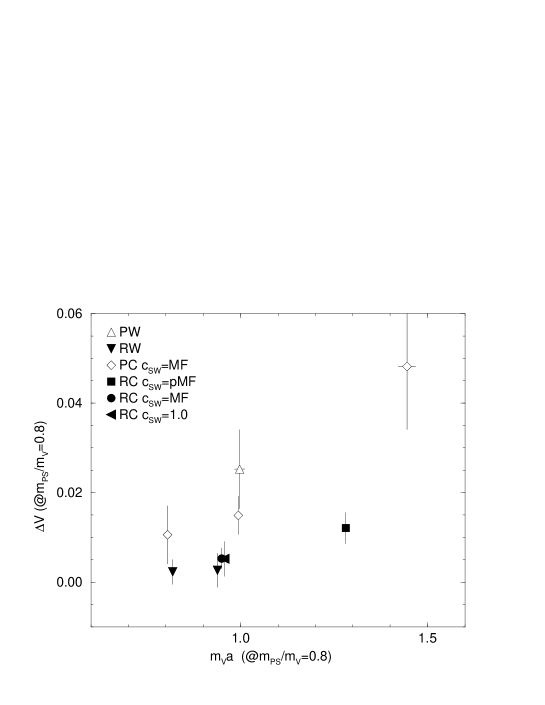
FIG. 6.: ${\Delta}V$ as a function of the vector meson mass $m_{\rm V}a$ at $m_{\rm PS}/m_{\rm V}=0.8$.

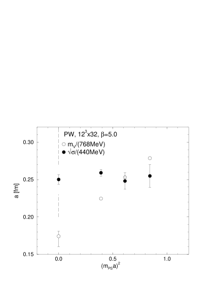
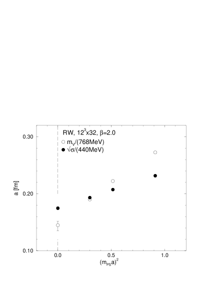
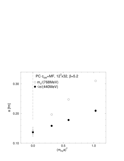
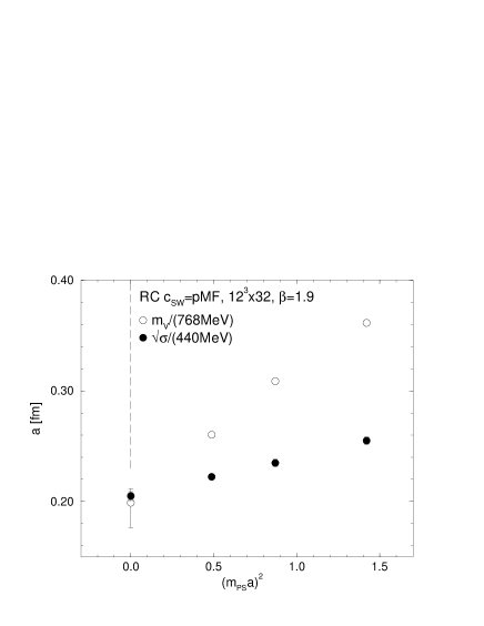
FIG. 7.: Lattice spacing in physical units as calculated from $m_{\rm V}a/768$ MeV and $\sqrt{\sigma}a/440$ MeV as function of $(m_{\rm PS}a)^{2}$. Values in the chiral limit are also shown.

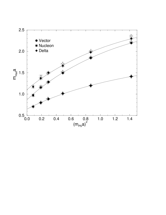
FIG. 8.: Chiral extrapolation of hadron masses as function of $(m_{\rm PS}a)^{2}$ for the RC_pMF action at $\beta=1.9$. Open symbols are results obtained on the $12^{3}\!\times\!32$ lattice whereas filled symbols are from the $16^{3}\!\times\!32$ lattice. Lines are fits to the results for the larger volume.

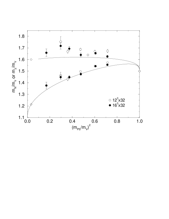
FIG. 9.: $m_{\rm N}/m_{\rm V}$ and $m_{\Delta}/m_{\rm V}$ as function of $(m_{\rm PS}/m_{\rm V})^{2}$ for the two runs with the RC_pMF action at $\beta=1.9$.

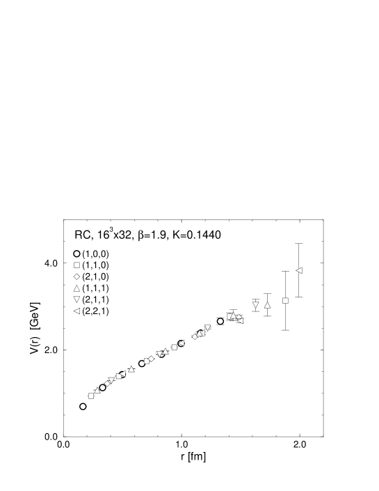
FIG. 10.: Static quark potential on the $16^{3}\!\times\!32$ lattice at the lightest sea quark mass $m_{\rm PS}/m_{\rm V}\approx 0.4$. The scale is set by $a_{\rho}$ in the chiral limit.

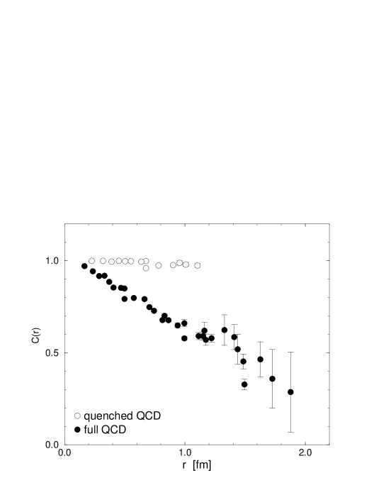
FIG. 11.: Overlap function $C(R)$ for full and quenched QCD as a function of $r$. Filled symbols are the data in full QCD on the $16^{3}\!\times\!32$ lattice with the RC_pMF action at $\beta=1.9$ and $K=0.1440$. Open symbols represent data in quenched QCD on a $9^{3}\!\times\!18$ lattice with the RG improved gauge action at $\beta=2.1508$ ($a^{-1}\approx 1$ GeV).