FSU-SCRI-99-04
Approach to the Continuum Limit of the Quenched Hermitian Wilson–Dirac Operator

Abstract

We investigate the approach to the continuum limit of the spectrum of the Hermitian Wilson–Dirac operator in the supercritical mass region for pure gauge SU(2) and SU(3) backgrounds. For this we study the spectral flow of the Hermitian Wilson–Dirac operator in the range $0\leq m\leq 2$. We find that the spectrum has a gap for $0<m\leq m_{1}$ and that the spectral density at zero, $\rho(0;m)$, is non-zero for $m_{1}\leq m\leq 2$. We find that $m_{1}\rightarrow 0$ and, for $m\neq 0$, $\rho(0;m)\rightarrow 0$ (exponential in the lattice spacing) as one goes to the continuum limit. We also compute the topological susceptibility and the size distribution of the zero modes. The topological susceptibility scales well in the lattice spacing for both SU(2) and SU(3). The size distribution of the zero modes does not appear to show a peak at a physical scale.

I Introduction

Continuum gauge field theory works under the assumption that all fields are smooth functions of space–time. This assumption is certainly a valid one for quantum gauge field theories that respect gauge invariance: One should always be able to fix a gauge so that the gauge fields are smooth functions of space–time since the action that contains derivatives in gauge fields will not allow it otherwise. The space of smooth gauge fields typically has an infinite number of disconnected pieces where the number of pieces is in one to one correspondence with the set of integers [1]. Every gauge field in each piece can be smoothly interpolated to another gauge field in the same piece but there is no smooth interpolation between gauge fields in different pieces. This is the case for U(1) gauge fields in two dimensions and SU(N) gauge fields in four dimensions.

In lattice gauge theory, gauge fields are represented by link variables $U_{\mu}(x)$ that are elements of the gauge group. Continuum derivatives are replaced by finite differences and the concept of smoothness of gauge fields does not apply. Any lattice gauge field configuration, $U_{\mu}(x)=e^{iA_{\mu}(x)}$ can be deformed to the trivial gauge field configuration by the interpolation $U_{\mu}(x;\tau)=e^{i\tau A_{\mu}(x)}$ with $U_{\mu}(x;1)=U_{\mu}(x)$ and $U_{\mu}(x;0)=1$. Since smoothness does not hold on the lattice away from the continuum limit, the space of gauge fields on the lattice forms a simply connected space. Separation of the gauge field space into an infinite number of disconnected pieces can only be realized in the continuum limit.

In this paper, we will address the following basic question: Do we see a separation of lattice gauge fields configurations into topological classes as we approach the continuum limit? To answer this question, we will use several ensembles of lattice gauge field configurations obtained from pure SU(2) and SU(3) gauge field theory. We will use a Wilson–Dirac fermion to probe the lattice gauge field configuration. Our motivation is the overlap formalism [2] for chiral gauge theories. Topological aspects of the background gauge field are properly realized by the chiral fermions in this formalism and therefore it provides a good framework to answer the above question. The hermitian Wilson–Dirac operator enters the construction of lattice chiral fermions in the overlap formalism and topological properties of the gauge fields are studied by looking at the spectral flow of the hermitian Wilson–Dirac operator as a function of the fermion mass. Contrary to some other approaches to investigate the topological properties of lattice gauge field configurations [3] we do not modify the gauge fields, generate by some Monte Carlo procedure, in any way.

The paper is organized as follows. We begin by explaining in Section II the connection between the spectral flow of the hermitian Wilson–Dirac operator and the topological content of the background gauge field. Possible scenarios for the qualitative nature of the spectrum on the lattice are presented. In Section III we present numerical results on the spectral properties of lattice gauge field ensembles and their behavior as the continuum limit is approached. Results for the topological susceptibility in pure SU(2) and SU(3) gauge theory computed using the overlap definition of the topological charge are shown in Section IV. We also present results on the size distribution of the zero modes of the Hermitian Wilson–Dirac operator.

II Spectral flow, topology and condensates

The massless Dirac operator in the continuum anticommutes with $\gamma_{5}$. Therefore, the non-zero imaginary eigenvalues of the massless Dirac operator come in pairs, $\pm i\lambda$, with $\psi$ and $\gamma_{5}\psi$ being the two eigenvectors. The zero eigenvalues of the massless Dirac operator are also eigenvalues of $\gamma_{5}$. These chiral zero modes are a consequence of the topology of the background gauge field. It is useful to consider the spectral flow of the Hermitian Dirac operator:

$${\bf\rm H}(m)=\gamma_{5}(\gamma_{\mu}D_{\mu}-m)$$ (1)

The non-zero eigenvalues of the massless Dirac operator combine in pairs to give the following eigenvalue equation:

$${\bf\rm H}(m)\chi_{\pm}=\lambda_{\pm}(m)\chi_{\pm}=\pm\sqrt{\lambda^{2}+m^{2}}\chi_{\pm}~{}.$$ (2)

$\chi_{\pm}$ are linear combinations of $\psi$ and $\gamma_{5}\psi$. The eigenvalues $\lambda_{\pm}(m)$ of these modes never cross the x-axis in the spectral flow of ${\bf\rm H}(m)$ as a function of $m$. The zero eigenvalues, $\gamma_{\mu}D_{\mu}\phi_{\pm}=0$ with $\gamma_{5}\phi_{\pm}=\pm\phi_{\pm}$ result in

$${\bf\rm H}(m)\phi_{\pm}=\mp m\phi_{\pm}$$ (3)

These modes, associated with topology, result in flow lines that cross the x-axis. A positive slope corresponds to negative chirality and vice-versa. The net number of lines crossing zero (the difference of positive and negative crossings) is the topology of the background gauge field. Global topology of gauge fields cause exact zero eigenvalues at $m=0$. In addition, one can have a non-zero spectral density at zero. In an infinite volume in the continuum, the spectrum is continuous and $\rho(\lambda;m)d\lambda$ is the number of eigenvalues in the infinitesimal region $d\lambda$ around $\lambda$. The spectral gap $\lambda_{g}(m)$ defined as the lowest eigenvalue at $m$ is equal to $|m|$. The spectral density at zero, $\rho(0;m)$, can be non-zero only at $m=0$ indicating spontaneous chiral symmetry breaking in a theory like QCD. The continuum picture is shown in Fig. 1.

FIG. 1.: Continuum picture of the spectral gap and the spectral density at zero.

To study the possible emergence of the above picture as the continuum limit of a lattice gauge theory picture, we need to have a lattice realization of ${\bf\rm H}(m)$. It is important to note that we are interested in the spectral flow of a single Dirac fermion. With this in mind, we choose the hermitian Wilson–Dirac operator obtained by multiplying the standard Wilson–Dirac operator by $\gamma_{5}$:

$${\bf\rm H}_{L}(m)=\pmatrix{{\bf\rm B}(U)-m&{\bf\rm C}(U)\cr{\bf\rm C}^{\dagger}(U)&-{\bf\rm B}(U)+m\cr}.$$ (4)

${\bf\rm C}$ is the naive lattice first derivative term and ${\bf\rm B}$ is the Wilson term. We are interested in the spectral flow of ${\bf\rm H}_{L}(m)$ as a function of $m$. We note that $m=0,2,4,6,8$ are the points where the free fermions become massless with degeneracies $1,4,6,4,1$ respectively. Next we observe that ${\bf\rm H}_{L}(m)$ can have a zero eigenvalue only if $m>0$ [4].

FIG. 2.: Possible scenarios of the spectral gap and the spectral density at zero on the lattice.

We focus on the range $0\leq m\leq 2$ and propose the following scenarios for the spectral gap and the spectral density at zero on the lattice and their approach to the continuum limit. Six different, but not completely independent scenarios are possible as shown in Fig. 2.

• On the lattice we have (a) and (i) with $m_{c}\rightarrow 0$ in the continuum limit. $\rho(0;m_{c})$ approaches the continuum limit with proper scaling taken into account.

• On the lattice we have (b) and (ii) where (a) and (i) are the continuum limit. In this case, $m_{1}\rightarrow 0$ and $m_{2}\rightarrow 0$. In the limit we also get $\rho(0;0)$.

• On the lattice we first have (c) and (ii) going, at weaker coupling to (b) and (ii), where (a) and (i) are the continuum limit. The gap opens up at some $m_{2}>m_{1}$ at some coupling and afterwards the approach to the continuum is as in the previous scenario.

• On the lattice we have (c) and (ii) where (c) and (i) are the continuum limit. In this case, $m_{1}\rightarrow 0$. However, the gap does not open up for $m>0$ in the continuum limit.

• On the lattice we first have (c) and (iii), going to (b) and (ii) at some coupling. Afterwards, the approach to the continuum limit is again as in the second scenario.

• On the lattice we have (c) and (iii) where (c) and (i) are the continuum limit. Here also $m_{1}\rightarrow 0$ and $\rho(0;m)=0$ if $m>0$. However, the gap does not open up for $m>0$.

We will show that numerical studies of the spectral flow on various ensembles favor the last scenario. Before we do that, we present a topological argument which will show that zero eigenvalues of ${\bf\rm H}_{L}(m)$ can occur anywhere in the region $0<m<8$ [5]. The spectrum of ${\bf\rm H}_{L}(m)$ and $-{\bf\rm H}_{L}(8-m)$ are identical for an arbitrary gauge field background. Since zero eigenvalues can occur only for $m>0$ in ${\bf\rm H}_{L}(m)$, it follows that zero eigenvalues can occur only in the region $0<m<8$. It also follows that every level crossing zero from above in the spectral flow of ${\bf\rm H}_{L}(m)$ must be accompanied by a level crossing zero from below. In a single instanton background a level crossing zero from above at $m_{+}$ is accompanied by another level crossing zero from below at $2>m_{-}>m_{+}$. The second crossing is due to one of the four doubler modes. Both $m_{\pm}$ will be functions of the size of the instanton $\rho$ in lattice units. For $\rho>>a$, $m_{+}\approx 0$ and $m_{-}\approx 2$. As $\rho$ decreases, $m_{+}$ moves farther away from zero and $m_{-}$ moves away from $2$ and closer to $m_{+}$. This motion as a function of $\rho$ is smooth and for some value of $\rho$, $m_{+}=m_{-}$. The spectral flow changes smoothly as the configuration is changed slowly. As we move in configuration space the topological charge of a configuration changes. Tracing the spectral flow as a function of configurations shows that zero eigenvalues of ${\bf\rm H}_{L}(m)$ can occur anywhere in the region $0<m<8$.

III Spectral density at zero

In the previous section, we argued that ${\bf\rm H}_{L}(m)$ can have zero crossings anywhere in the region $m_{1}\leq m\leq 2$. Therefore the spectral gap is zero in this region on the lattice. This has direct implications for how the spectral density at zero behaves on the lattice. A careful study of the spectral density at zero has been performed on a variety of SU(3) pure gauge ensembles. This is done by computing the low lying eigenvalues of ${\bf\rm H}_{L}(m)$ using the Ritz functional [6]. The low lying eigenvalues over the whole ensemble are then used to obtain the integral of the spectral density function, $\int_{0}^{\lambda}\rho(\lambda^{\prime};m)d\lambda^{\prime}$. A linear fit in $\lambda$ is made, and $\rho(0;m)$ is obtained as the coefficient of the linear term.

FIG. 3.: $\rho(0;m)$ as a function of $m$ for various SU(3) pure gauge ensembles at gauge couplings $\beta=6.0$, $5.85$ and $5.7$.

All ensembles show a peak in $\rho(0;m)$ at some value of $m$ near $m_{1}$. There is a sharp rise to the peak from the left and a gradual fall from the peak on the right. There is a gradual rise again to a second peak at the location of the first set of doublers. The peak itself gets sharper and moves to the left as one goes toward the continuum limit. $\rho(0;m)$ is non-zero for $m_{1}\leq m\leq 2$ in the infinite volume limit at any finite value of the lattice gauge coupling (see below). $m_{1}$ goes to zero as the lattice coupling approaches the continuum. $\rho(0;m)$ approaches the infinite lattice volume limit from below as expected. We are fairly confident that we have the infinite volume limit estimate for $\rho(0;m)$ at all the lattice spacings plotted in Fig. 3.

In Fig. 4 and Fig. 5, we focus on the behavior of $\rho(0;m)$ at a fixed $m$ as one approaches the continuum limit. In Figure 4 we plot $\rho(0;m)$ as a function of the lattice spacing measured in units of the square root of the string tension (the values for the string tension are taken from Ref. [7]). In this figure $\rho(0;m)$ appears to go to zero exponentially in the inverse lattice spacing. This is given some credence by plotting the same figure in a logarithmic scale in Fig. 5 where the data is shown for several values of $m$. For $\beta=5.7$, the peak in $\rho(0;m)$ is quite close to $m=1.2$ as can be seen in Fig. 3, resulting in a large value for $\rho(0;1.2)$.

We remark that the $\rho(0;m)$ plotted in Fig. 5 seem to favor a functional form fitting $be^{-c/\sqrt{a}}$ for each $m$. The power of $a$ in the exponent is a consequence of an empirical fit but the data presents substantial evidence for the following: $\rho(0;m)$ in the supercritical mass region is non-zero for all finite lattice spacings. The approach to zero at zero lattice spacing is faster than any power of the lattice spacing. This shows that the last scenario presented in the previous section is favored by our numerical results.

FIG. 4.: The approach of $\rho(0;1.7)$ to the continuum limit as a function of the lattice spacing in units of the string tension for $\beta=5.7$, $5.85$, $6.0$, $6.1$, $6.2$ and $6.3$.

FIG. 5.: The approach of $\rho(0;m)$ to the continuum limit as a function of $1/\sqrt{a\sqrt{\sigma}}$ for $m=1.2$ (diamonds) $1.5$ (octagons) and $1.7$ (crosses). For $m=1.2$ only values at $\beta\leq 6.0$ are shown.

IV Topological susceptibility

In addition to studying $\rho(0;m)$, we also looked at the density of levels crossing zero in an infinitesimal range $dm$ centered at $m$. In the continuum we expect levels crossing zero only at $m=0$, but on the lattice we find a finite density of levels crossing zero wherever $\rho(0;m)$ is non-zero on the lattice. The overlap formalism for constructing a chiral gauge theory on the lattice [2] provides a natural definition of the index, $I$, of the associated chiral Dirac operator. The index is equal to half the difference of negative and positive eigenvalues of the hermitian Wilson–Dirac operator. A simple way to compute the index $I$ is to compute the lowest eigenvalues of ${\bf\rm H}_{L}(m)$ at some suitably small $m$ before any crossings of zero occurred. Then $m$ is slowly varied and the number and direction of zero crossings are tracked. The net number at some $m_{t}$ is the index of the overlap chiral Dirac operator. Since crossings occur for all values of $m$ in the range $m_{1}\leq m\leq 2$, the topological charge of a lattice gauge field configuration defined as the net level crossings in ${\bf\rm H}_{L}(m)$ in the range $[0,m_{t}]$ will depend on $m_{t}$.

The topology of a single lattice gauge field configuration is not interesting in a field theoretic sense. One has to obtain an ensemble average of the topological susceptibility and study its dependence on $m$. This has been done on a variety of ensembles and the results show that the topological susceptibility is essentially independent of $m$ in the region to the left of the peak in $\rho(0;m)$. A detailed study of the SU(3) ensemble at $\beta=6.0$ on a $16^{3}\times 32$ lattice presented in Figure 6 illustrates this point. In the first line is shown the density of zero eigenvalues $\rho(0;m)$ and the number of crossings in each mass bin. We see that $\rho(0;m)$ rises sharply in $m$, then falls to a nonzero value where there is a small number of levels crossing zero. In the second line of Figure 6, we show the size of the zero modes $\rho_{z}(m)$. We define a size of the eigenvector associated with the level crossing zero mode as

$$\rho_{z}(m)={\frac{1}{2}}{{\sum_{t}f(t)}\over{f_{\rm max}}}\quad f(t)=\sum_{\vec{x}}{\rm tr}(\phi^{\dagger}({\vec{x}},t)\phi({\vec{x}},t))$$

where $\phi(\vec{x},t)$ is the eigenvector of ${\bf\rm H}_{L}$ at the crossing point and $f_{max}$ is the maximum value of $f(t)$ over $t$. Another definition based on the second moment of $f(t)$ was used in Ref. [8]. We should emphasize that we look only at the sizes of eigenmodes that cross, and only close to the crossing point. Only then can we expect to get a good estimate of the localization size inspired by the ’t Hooft zero mode. The modes are large near $m_{1}$ where $\rho(0;m)$ is large, then $\rho_{z}(m)$ drops sharply to about $1$ or $2$ lattice spacings and stays there up to $m=2$. We see that the corresponding topological susceptibility rises sharply when $\rho_{z}(m)$ is large for $m$ near $m_{1}$ and then it is quite stable when $\rho_{z}(m)$ is small. This result shows that while the index, $I$, of the field is $m$ dependent, the topological susceptibility, $\chi$ (a physical quantity) is independent of the contribution from the small modes for $m\mathrel{\hbox to0.0pt{\lower 3.0pt\hbox{$\mathchar 536\relax$}\hss}\raise 2.0pt\hbox{$\mathchar 318\relax$}}1$.

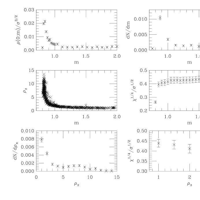
FIG. 6.: Detailed study for $\beta=6.0$, $16^{3}\times 32$.

To further clarify the relative contribution of the zero modes, in the last line of Figure 6 the zero mode size distribution is plotted as a function of $\rho_{z}$. In the adjacent graph, the topological susceptibility, $\chi$, here defined by the contribution of zero modes of size $\rho_{z}$ and larger, is stable when $\rho_{z}<2$. Hence, the small modes do not affect the estimate of $\chi$ even though there is an abundance of such modes. Our estimates of $\chi$ are shown in Table I where we use the string tension value $\sqrt{\sigma}=440$ MeV to set the scale. Our results are in rough agreement with other groups [9] and also show good evidence for scaling.

TABLE I.: Topological susceptibility and parameters for $SU(3)$ and $SU(2)$.

	$\beta$	size	$N_{\rm conf}$	$\chi^{1/4}$(MeV)
	$6.0$	$16^{3}\times 32$	75	194(10)
$SU(3)$	$5.85$	$8^{3}\times 16$	200	198(05)
	$5.7$	$8^{3}\times 16$	50	193(10)
	$2.6$	$16^{4}$	400	229(05)
$SU(2)$	$2.5$	$16^{4}$	100	232(10)
	$2.4$	$16^{4}$	200	220(06)

V Size distribution of zero modes

Studies in smooth gauge field backgrounds on the lattice have shown that single instantons result in a single level crossing zero at some $m$ in the region $[0,2]$ where the shape of the mode at the crossing is a good representation of the shape of the instanton [5]. Similarly, there is a pair of levels crossing zero (one from above and another from below) when the gauge field background has an instanton and anti-instanton. Again, the shape of the modes at the crossing points are good representations of the instanton and anti-instanton. This motivates us to look at the size distribution of the zero modes of the Hermitian Wilson-Dirac operator on the lattice. Since lattice gauge fields generated in typical Monte Carlo simulations are rough, the correspondence between zero modes and topological objects might be questionable – the existence of topological objects (a collection of instantons and anti-instantons) “underneath” the typically large quantum fluctuations is somewhat questionable as well. However, levels crossing zero contribute to the global topology and an analysis of the size distribution of the zero modes is therefore interesting. Such size distributions are shown in Figure 7 for gauge group SU(2). All distributions show a sharp rise at small sizes due to the abundance of small zero modes that occur in the bulk of the region $m_{1}\leq m\leq 2$. These modes do not affect the computation of the topological susceptibility and can be viewed as being due to the ultra-violet fluctuations in the gauge field background. If we eliminate the small modes from the distribution, the size distribution at $\beta=2.4$ on the $16^{4}$ lattice shows some evidence for a broad peak around $\rho_{z}=0.6$ fm. One should keep in mind that the box size is roughly $1.92$ fm and the peak is occurring at a value which is roughly a third of the box. It is tempting to explain this peak as a finite volume effect. Some support for this explanation is provided by looking at the distributions at $\beta=2.5$ and $\beta=2.6$ on a $16^{4}$ lattice. These boxes are now roughly $1.38$ fm and $0.98$ fm, respectively. After discarding the small zero modes, both the distributions show a broad peak at roughly $\rho_{z}=0.45$ fm and $\rho_{z}=0.3$ fm, respectively. As in the $\beta=2.4$ case these peaks occur at roughly a third of the box size and the magnitude of the peak is larger as one goes to weaker coupling for a fixed lattice volume. This is quite consistent with the peak being a finite volume effect. In Fig. 8 we show all the SU(2) size distributions together plotted in lattice units. There is evidence for a broad peak at roughly $5$ lattice units – roughly a third of the lattice box size. Therefore, we conclude that the size distribution of zero modes does not show evidence for a peak at a physical scale even after we remove the small modes which are most likely lattice artifacts. We have to conclude that it is not possible to relate the size analysis of the zero modes carried out here to a size distribution of topological objects as it is postulated for the instanton liquid model of QCD [10].

FIG. 7.: Size distribution of zero modes on various SU(2) ensembles.

FIG. 8.: Size distribution of zero modes on the SU(2) ensembles plotted in lattice units. The crosses correspond to $\beta=2.4$, the diamonds $\beta=2.5$, and the squares $\beta=2.6$. All lattice sizes are $16^{4}$.

The conclusions remain the same for the various SU(3) ensembles that we studied. The size distributions are plotted in Figure 9. The $\beta=5.7,\ 5.85\ {\rm and}\ 6.0$ ensembles come from lattices with linear extent roughly equal to $1.4$ fm, $1.04$ fm and $1.6$ fm, respectively. Clearly the size distribution on the $\beta=5.85$ ensemble suffers strongly from finite volume effects whereas the $\beta=6.0$ ensemble is not affected as much. We should remark that we do not see any evidence for a finite volume effect in the computation of the topological susceptibility. This is probably because the size distribution of the individual zero modes is not that relevant for the global topology which only depends in principle on the net number of level crossings and not on the size and shape of these crossing modes.

VI Discussion

A probe of pure lattice gauge field ensembles using Wilson fermions has revealed that the gauge fields are not continuum like on the lattice at gauge couplings that are typically considered to be weak. If they were continuum like, we should have seen evidence that $\rho(0;m)$ is non-zero at a single value of $m$ or in a region in $m$ that is of the order of the lattice spacing. Furthermore, we should have seen a symmetry in the spectrum at values of $m$ on either side of the point (or region) where $\rho(0;m)$ is non-zero. Instead, we found that $\rho(0;m)$ is non-zero in a region $m_{1}\leq m\leq 2$. In the continuum limit, there is evidence that $m_{1}$ goes to zero and that $\rho(0;m)$ goes to zero away from $m=0$. However, the spectral distribution does not show evidence for a symmetry as $m\rightarrow-m$.

FIG. 9.: Size distribution of zero modes on various SU(3) ensembles.

A remark on the approach of $\rho(0;m)$ to the thermodynamic limit at a fixed lattice gauge coupling is in order. For a small lattice, with linear size of the order of the extent $N_{t}$ for which the finite temperature deconfinement transition occurs at the given gauge coupling, the number of very small eigenvalues of the Wilson-Dirac operator will be essentially zero. When the lattice size is increased this number will grow rapidly, leading, for a while, to a rapid increase in the extracted estimate of $\rho(0;m)$ and then leveling off at the infinite volume value of $\rho(0;m)$. We found that this happens for a linear size about twice the extent $N_{t}$ mentioned above.

The density of level crossing zero modes, $dN/dm$, of the Hermitian Wilson–Dirac operator is in accordance with the behavior of $\rho(0;m)$. In spite of a large number of levels crossing zero in the bulk of $m_{1}\leq m\leq 2$, we found that the topological susceptibility is unchanged by these small localized modes. We therefore interpret them as due to ultra-violet fluctuations. The size distribution of the zero modes is dominated by these small modes. However, the distribution, after we remove these small modes, does not show any clear peak at a physical scale. Some broad peaks we see in are explained as a consequence of finite volume effects.

We finally remark that all our studies in this paper have been on pure gauge field ensembles. There is a prediction for the spectral distribution of the Wilson-Dirac operator in full QCD using a continuum chiral lagrangian [11]. The prediction resembles the second scenario presented in section II and is qualitatively different from the result we have obtained for pure gauge ensembles. It would be interesting to test this prediction by numerical simulations of full QCD with Wilson fermions in the supercritical region. There is, however, a technical problem in using standard Hybrid Monte Carlo type algorithms for such simulations: the system will be locked in a single topological sector (with topology defined as half the difference of negative and positive eigenvalues of the hermitian Wilson-Dirac operator at the supercritical mass, $m_{d}$, where the simulation is carried out). This is due to the fact that a change in topology will require a change of net level crossings in the region $0<m<m_{d}$. However, the spectral flow has to be smooth as we update the configurations using classical dynamics in HMC type algorithms. Therefore, at some point in the change of topology the level crossing would need to occur at $m_{d}$, but such a configuration has a vanishing fermion determinant and hence can not be reached. Modifications of the HMC algorithm to circumvent this problems would need to be developed before a study of the spectral flow in full QCD in the supercritical region can be attempted.

REFERENCES

- [1] T. Eguchi, P.B. Gilkey and A.J. Hanson, Phys. Rep. 66 (1980) 213.
- [2] R. Narayanan and H. Neuberger, Nucl. Phys. B443 (1995) 305.
- [3] See, for example, M. Teper, hep-lat/9711011 and hep-th/9812187, P. van Baal, Nucl. Phys. B (Proc. Suppl.) 63 (1998) 127, and references therein.
- [4] R. Narayanan and H. Neuberger, Phys. Rev. Lett 71 (1993) 3251.
- [5] R.G. Edwards, U.M. Heller and R. Narayanan Nucl. Phys. B522 (1998) 285.
- [6] B. Bunk, K.Jansen, M. Lüscher and H. Simma, DESY Report (September 1994); T. Kalkreuter and H. Simma, Comput. Phys. Commun. 93 (1996) 33.
- [7] R.G. Edwards, U.M Heller, T.R. Klassen, Nucl. Phys. B517 (1998) 377.
- [8] R.G. Edwards, U.M Heller, R. Narayanan, R.L. Singleton, Jr., Nucl. Phys. B518 (1998) 319; R.G. Edwards, U.M. Heller and R. Narayanan, Nucl. Phys. B535 (1998) 403.
- [9] B. Alles, M. D’Elia and A. Di Giacomo, Nucl. Phys. B494 (1997) 281. T. DeGrand, Anna Hasenfratz, Tamas Kovacs, hep-lat/9801037; P. de Forcrand, M.G. Perez, J.E. Hetrick, I-O. Stamatescu, hep-lat/9802017.
- [10] T. Schafer, E. Shuryak, Rev. Mod. Phys. 70 (1998) 323.
- [11] S. Sharpe and R. Singleton, Jr., Phys. Rev. D58 (1998) 074501.