Random Matrix Theory and Chiral Logarithms

Abstract

Recently, the contributions of chiral logarithms predicted by quenched chiral perturbation theory have been extracted from lattice calculations of hadron masses. We argue that a detailed comparison of random matrix theory and lattice calculations allows for a precise determination of such corrections. We estimate the relative size of the $m\log(m)$, $m$, and $m^{2}$ corrections to the chiral condensate for quenched SU(2).

PACS: 11.30.Rd; 11.15.Ha; 12.38.Gc; 05.45.-a
Keywords: chiral perturbation theory; random matrix theory; lattice gauge calculations; scalar susceptibilities; SU(2) gauge theory

, , , , , , and

The identification of logarithmic corrections in the quark mass predicted by quenched chiral perturbation theory [1, 2] in lattice gauge results is a long standing problem. It seems that the latest numerical results [3, 4, 5, 6] on hadron masses in quenched lattice simulations allow for an approximate determination of these $\log(m)$ contributions. The determination of these logarithms is an important test of chiral perturbation theory which in turn plays a central role for the connection of low-energy hadron theory on one side and perturbative and lattice QCD on the other.

In a completely independent development, it has been shown by several authors that chiral random matrix theory (chRMT) is able to reproduce quantitatively microscopic spectral properties of the Dirac operator obtained from QCD lattice data (see the reviews [7, 8] and Refs. [9, 10, 11, 12]). Moreover, the limit up to which the microscopic spectral correlations can be described by random matrix theory (the analogue of the “Thouless energy”) was analyzed theoretically in [13, 14] and identified for quenched SU(2) lattice calculations in [15].

The following analysis uses the scalar susceptibilities, so we first give their definitions. The disconnected susceptibility is defined on the lattice by

$$\chi^{\rm disc}_{\rm lattice}=\frac{1}{N}\left\langle\sum_{k,l=1}^{N}\frac{1}{({\rm i}\lambda_{k}+m)({\rm i}\lambda_{l}+m)}\right\rangle-\frac{1}{N}\left\langle\sum_{k=1}^{N}\frac{1}{{\rm i}\lambda_{k}+m}\right\rangle^{2}\;,$$ (1)

where $N=L^{4}$ denotes the number of lattice points and the $\lambda_{k}$ are the Dirac eigenvalues. After rescaling the susceptibility by $N\Sigma^{2}$ ($\Sigma=$ absolute value of the chiral condensate for infinite volume and vanishing mass) chRMT predicts

$$\frac{\chi^{\rm disc}_{\rm RMT}}{N\Sigma^{2}} = 4u^{2}\int_{0}^{1}\d s\>s^{2}K_{0}(2su)\int_{0}^{1}\d t\>I_{0}(2stu)\bigg{\{}s(1-t^{2})$$ (3)

$$\qquad{}+4K_{0}(2u)[I_{0}(2su)+tI_{0}(2stu)]-8stI_{0}(2stu)K_{0}(2su)\bigg{\}}$$

$$\qquad{}-4u^{2}K_{0}^{2}(2u)\left[\int_{0}^{1}\d s\>I_{0}(2su)\right]^{2}$$

$$= 1-K_{0}(2u)I_{0}(2u)+[K_{0}(2u)-2uK_{1}(2u)]\int_{0}^{1}\d t\>I_{0}(2tu)$$

$$\qquad{}-\Bigg{\{}2uK_{0}(2u)\int_{0}^{1}\d t\>I_{0}(2tu)$$

$$\qquad{}-2u[K_{0}(2u)I_{0}(2u)+K_{1}(2u)I_{1}(2u)]\Bigg{\}}^{2}\;,$$

where the rescaled mass parameter $u$ is given by $u=m\Sigma L^{4}$. (For details we refer to [15].)

We shall also use the connected susceptibility which is defined on the lattice by

$$\chi^{\rm conn}_{\rm lattice}=-\frac{1}{N}\left\langle\sum_{k=1}^{N}\frac{1}{({\rm i}\lambda_{k}+m)^{2}}\right\rangle\;.$$ (4)

The chRMT result reads

$$\frac{\chi^{\rm conn}_{\rm RMT}}{N\Sigma^{2}}=4uK_{1}(2u)\int_{0}^{1}\d s\>(1-s)I_{0}(2su)\;.$$ (5)

Fig. 1 presents the deviation of the (parameter-free) random matrix prediction from the lattice result, more precisely the ratio

$${\bf ratio}=\left(\chi_{\rm lattice}-\chi_{\rm RMT}\right)/\left(\chi_{\rm RMT}\right)\;,$$ (6)

where $\chi$ can either be the disconnected (only this choice was investigated in [15]) or the connected susceptibility.

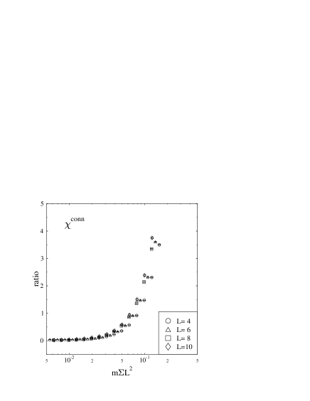
Figure 1: The ratio of Eq. (6) for the scaled susceptibilities plotted versus $m\Sigma L^{2}$ (in lattice units) for $\beta=2.0$ and four different lattice sizes, $N=4^{4}$, $6^{4}$, $8^{4}$, and $10^{4}$.

The motivation for investigating ${\bf ratio}$ rather than $\chi_{\rm lattice}$ itself is that in Eq. (6) finite size corrections cancel to a remarkable degree, allowing us to use data from smaller $m$ values. We have seen in Fig. 2 of [16] that the knowledge of finite size effects which we gain from RMT allows us to find the thermodynamic limit of the chiral condensate from extremely small lattices. This can also be formulated in the following way: for a given value of ${\bf ratio}$ in Fig. 1, the finite size corrections for all four lattice sizes are expected to be similar, as the corresponding values of $m_{\pi}^{2}L^{2}\propto mL^{2}$ are very close, which is why we have plotted ${\bf ratio}$ against $m\Sigma L^{2}$ in Fig. 1.

What do we expect beyond the Thouless energy? Then, the lattice is large enough so that the valence pion, which is the lightest particle, fits on the lattice. Naturally, all other particles also fit on the lattice, and therefore we expect that the chiral condensate and the two susceptibilities will rapidly approach their thermodynamic limit.

For a finite lattice and a non-vanishing mass, the chiral condensate is given by

$$\sigma_{\rm lattice}(m)=\frac{1}{N}\left\langle\sum_{k=1}^{N}\frac{1}{{\rm i}\lambda_{k}+m}\right\rangle\;.$$ (7)

In the quenched theory, the connected susceptibility is given simply by

$$\chi^{\rm conn}(m)=\frac{\partial}{\partial m}\sigma(m)\;,$$ (8)

so we can find the infinite-volume behavior of $\chi^{\rm conn}$ from that of $\sigma$. We expect from chiral perturbation theory [17] that the chiral condensate has the form

$$\sigma(m)=\Sigma\left[1-Am\log(m)+Bm+\frac{1}{2}Cm^{2}+\cdots\right]\;.$$ (9)

Eq. (9) requires several comments. In the continuum, quenched chiral perturbation theory predicts a leading term proportional to $\frac{\langle\nu^{2}\rangle}{L^{4}}\log(m)$, where $\langle\nu^{2}\rangle/L^{4}$ is the topological susceptibility [17, Sec. 7]. We argue that this leading term should be absent in our case. For finite lattice spacing the Atiyah–Singer-index theorem does not apply for staggered fermions. Therefore the role of topology has to be interpreted with care. We have seen in [11] that the small Dirac eigenvalues are well described by random matrix results for $\nu=0$. This means that the quasi-zero modes related to topology are shifted to such large values that they are not visible. (This is presumably due to discretization errors proportional to $a^{2}$, with $a$ the physical lattice spacing.) Thus the violation of axial symmetry which generates the logarithmic term in the quenched case is dominated by the explicit quark masses, which motivates Eq. (9). It would be very interesting to study the $\nu\neq 0$ sector for which we expect a leading $\log(m)$ term, which might require, however, very small $a$ and a large number of lattice points.

Eq. (9) implies that in the thermodynamic limit

$$\chi^{\rm conn}_{\rm lattice}=\Sigma\left[-A\log(m)-A+B+Cm+\cdots\right]\;.$$ (10)

On the other hand, the large-volume limit of the RMT susceptibility is

$$\chi^{\rm conn}_{\rm RMT}\rightarrow\frac{1}{4m^{2}L^{4}}\;.$$ (11)

Putting the two expressions together, we find that

$${\rm{\bf ratio}}\rightarrow(m\Sigma L^{2})^{2}\frac{4}{\Sigma}\left[-A\log(m)-A+B+Cm+\cdots\right]-1\;.$$ (12)

Strictly speaking, the $-1$ ought to be neglected in comparison with the first term as $L\to\infty$. However, we should be prepared to observe some sub-leading corrections in the data taken on finite lattices.

We have confronted Eq. (12) with lattice Monte Carlo data for two values of the coupling strength $\beta$, $\beta=2.0$ and $\beta=2.2$. The lattice sizes and numbers of configurations are given in Table 1.

Table 1: Lattice sizes and numbers of configurations for the lattice data.

$\beta=2.0$
L	4	6	8	10
# of configs	49978	24976	14290	4404
$\beta=2.2$
L	6	8	10	12
# of configs	22292	13975	2950	1388

To check Eq. (12) we did the following for both values of $\beta$:
We chose different values for ${\bf ratio}=b_{i}$ and determined the values of $m\Sigma L^{2}$ for which they were reached for our different lattice sizes. Let us denote these numbers by $Y(L,b_{i})$. Eq. (12) implies that

$$\frac{1}{Y(L,b_{i})^{2}}=r(b_{i})\left[-\log(m)+\frac{B}{A}-1+\frac{C}{A}m+\cdots\right]$$ (13)

where $r(b)$ will be proportional to $1/b$ as $b\to\infty$. Since we do not reach too large values of $b$, we used the ansatz

$$\frac{1}{Y(L,b_{i})^{2}}=\frac{q}{b_{i}+s}\left[-\log(m)+\frac{B}{A}-1+\frac{C}{A}m+\cdots\right]$$ (14)

to fit our data. In Eq. (14) not only $Y^{-2}$ has statistical errors, but also $m$. In our $\chi^{2}$ fit, however, only the errors of $Y^{-2}$ are taken into account.

Obviously, the values $Y(L,b_{i})$ for the same lattice size $L$ are highly correlated. It is, however, unclear how to calculate the correlations of these quantities, which are related to the original lattice results only in a rather implicit manner. Moreover, correlated fits tend to have problems [18]. Therefore we decided to ignore correlations completely, although this will lead to an underestimation of the errors on the fit parameters.

For the thermodynamic limit of the disconnected susceptibility we assume the same form as Eq. (10). In RMT, the large-volume limit is given by

$$\chi^{\rm disc}_{\rm RMT}\to\frac{1}{8m^{2}L^{4}}$$ (15)

so that the ansatz of Eq. (14) applies as well.

In Figs. 2 and 3 we plot $Y^{-2}$ versus $m$ together with the fits for $\beta=2.0$ and $2.2$, respectively. In the case of the connected susceptibility we used $b_{i}=2.0,3.0,4.0,5.0$ ($\beta=2.0$) and $b_{i}=5.0,6.0,7.0,8.0$ ($\beta=2.2$) and obtained the results of Table 2.

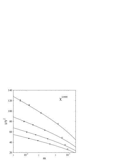
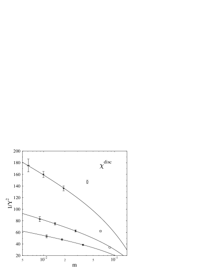
Figure 2: The value of $Y=m\Sigma L^{2}$ at $\beta=2.0$ for which $\mathbf{ratio}=b$ for various values of $b$ as a function of $m$. Larger values of $b$ belong to smaller values of $1/Y^{2}$. The rightmost filled dots correspond to $L=6$, the leftmost to $L=10$, whereas the open dots represent data for $L=4$, which were not used in the fit. All quantities are measured in lattice units.

Table 2: Fit parameters for the connected susceptibility.

$\beta$	$B/A$		$C/A$		$q$				$s$		$\chi^{2}/\mathrm{dof}$
2.0	2.29${}\pm{}$	0.63	$-5.97$${}\pm{}$	5.17	43	.9${}\pm{}$	4	.5	0.25${}\pm{}$	0.02	0.50
2.2	0.86${}\pm{}$	0.18	$-2.46$${}\pm{}$	1.86	486	${}\pm{}$	19		0.81${}\pm{}$	0.05	1.75

For the disconnected susceptibility we used $b_{i}=1.0,2.0,3.0$ ($\beta=2.0$) and $b_{i}=6.0,7.0,8.0$ ($\beta=2.2$) and found the values given in Table 3.

Figure 3: Same as Fig. 2 but for $\beta=2.2$ and with the dots, from left to right, corresponding to $L=12$, $10$, $8$, and $6$, respectively.

Table 3: Fit parameters for the disconnected susceptibility.

$\beta$	$B/A$			$C/A$				$q$		$s$		$\chi^{2}/\mathrm{dof}$
2.0	1.	9 ${}\pm{}$	3.1	$-12$	${}\pm{}$	32		31${}\pm{}$	16	0.05${}\pm{}$	0.05	0.02
2.2	$-1$.	45 ${}\pm{}$	0.48	18	.7${}\pm{}$	4	.1	569${}\pm{}$	127	$-0.60$${}\pm{}$	0.61	0.28

The main message of Figs. 2 and 3 is that without any doubt the data are not fitted by horizontal lines. This demonstrates the presence of additional contributions in the quark mass. The approximate linearity of the curves for small $m$ shows that the logarithmic contribution is the dominant one. For the connected susceptibility, the data are well fitted by the ansatz (9), i.e., with only the three leading corrections. For the disconnected susceptibility, our statistical precision does not allow for a precise determination of the ratios $B/A$ and $C/A$. For very small lattices ($4^{4}$ in Fig. 2) finite size effects seem to spoil our analysis.

It is clear from Figs. 2 and 3 that one would really like to have numerical simulations with substantially larger statistics and larger lattices. As the applicability of RMT to the description of the low-energy Dirac spectrum is by now well established we can limit ourselves in the future to the calculation of just the lowest eigenvalues instead of the complete spectrum. This should allow us to gain the necessary statistics.

To conclude, let us remark that the aim of this paper is primarily to draw attention to this new method to extract chiral logarithms and other corrections in the quark mass, and to stimulate the discussion of their interpretation. The obvious next step is to analyze the susceptibilities within the framework of quenched chiral perturbation theory.

References

- [1] C.W. Bernard and M.F.L. Golterman, Phys. Rev. D46 (1992) 853; hep-lat/9311070; Phys. Rev. D49 (1994) 486; M.F.L. Golterman, Acta Phys. Polon. B25 (1994) 1731.
- [2] J.N. Labrenz and S.R. Sharpe, Nucl. Phys. B (Proc. Suppl.) 34 (1994) 335; Phys. Rev. D54 (1996) 4595.
- [3] W. Bardeen, A. Duncan, E. Eichten, and H.B. Thacker, hep-lat/9809147.
- [4] M. Göckeler, R. Horsley, V. Linke, D. Pleiter, P.E.L. Rakow, G. Schierholz, A. Schiller, P. Stephenson, and H. Stüben, hep-lat/9810006.
- [5] R. Burkhalter, hep-lat/9810043.
- [6] R.D. Kenway, hep-lat/9810054.
- [7] For a recent review on random matrix theory in general, see T. Guhr, A. Müller-Groeling, H.A. Weidenmüller, Phys. Rept. 299 (1998) 189.
- [8] For a review on RMT and Dirac spectra, see the recent review by J.J.M. Verbaarschot, hep-th/9710114, and references therein.
- [9] J.J.M. Verbaarschot, Phys. Lett. B 368 (1996) 137.
- [10] M.A. Halasz and J.J.M. Verbaarschot, Phys. Rev. Lett. 74 (1995) 3920.
- [11] M.E. Berbenni-Bitsch, S. Meyer, A. Schäfer, J.J.M. Verbaarschot, and T. Wettig, Phys. Rev. Lett. 80 (1998) 1146.
- [12] J.-Z. Ma, T. Guhr, and T. Wettig, Euro. Phys. J. A 2 (1998) 87, 425.
- [13] R.A. Janik, M.A. Nowak, G. Papp, and I. Zahed, Phys. Rev. Lett. 81 (1998) 264.
- [14] J.C. Osborn and J.J.M. Verbaarschot, Phys. Rev. Lett. 81 (1989) 268; Nucl. Phys. B525 (1998) 738.
- [15] M.E. Berbenni-Bitsch, M. Göckeler, T. Guhr, A.D. Jackson, J.-Z. Ma, S. Meyer, A. Schäfer, H.A. Weidenmüller, T. Wettig, and T. Wilke, Phys. Lett. B 438 (1998) 14.
- [16] M.E. Berbenni-Bitsch, A.D. Jackson, S. Meyer, A. Schäfer, J.J.M. Verbaarschot, and T. Wettig, Nucl. Phys. B (Proc. Suppl.) 63 (1998) 820.
- [17] J.C. Osborn, D. Toublan and J.J.M. Verbaarschot, hep-th/9806110.
- [18] C. Michael and A. McKerell, Phys. Rev. D51 (1995) 3745.