BI-TP 99/1
FSU-SCRI-99-02
January 1999

Improved Staggered Fermion Actions for
QCD Thermodynamics

U. M. Heller^a, F. Karsch^b and B. Sturm^b

^a SCRI, Florida State University, Tallahassee, FL 32306-4130, USA

^b Fakultät für Physik, Universität Bielefeld, D-33615 Bielefeld, Germany

ABSTRACT

We analyze the cut-off dependence of the fermion contribution to the finite temperature free energy density in ${\cal O}(g^{2})$ lattice perturbation theory for several improved staggered fermion actions. Cut-off effects are drastically reduced for the Naik action and an action with improved rotational symmetry of the quark propagator. We show that improvement of rotational symmetry at ${\cal O}(g^{2})$ further reduces cut-off effects in thermodynamic observables. We also show that the introduction of fat-links does not have a significant influence on cut-off distortions at ${\cal O}(g^{2})$.

1 Introduction

During recent years much progress has been made in the analysis of the thermodynamics of $SU(N)$ gauge theories. Based on detailed studies of the cut-off dependence of thermodynamic observables in lattice regularized gauge theories an extrapolation of results for the equation of state to the continuum limit has been performed for the first time [1]. In addition, it could be shown that the influence of a finite lattice cut-off on thermodynamic observables is greatly reduced when improved actions such as ${\cal O}(a^{2})$ Symanzik improved [2] or tree level perfect [3] gauge actions are used. By construction tree level improved actions do reduce the cut-off dependence of thermodynamic observables in the infinite temperature, ideal gas limit of gauge theories [4, 5]. They do, however, also seem to reduce cut-off effects at non-zero values of the gauge coupling $g^{2}$, i.e. at finite temperature. Similar conclusions have been drawn from a first analysis of QCD thermodynamics with an improved staggered fermion action [6].

Using tree level improved gauge and fermion actions it is now possible to perform lattice calculations at finite temperature, which at least in the infinite temperature limit lead to acceptably small systematic cut-off errors. Numerical simulations for $SU(N)$ gauge theories as well as QCD with dynamical fermions [6] give some indications that this improvement carries over also into the temperature regime close to the deconfinement phase transition. This suggests that improved actions also show a reduced cut-off dependence at non-zero gauge coupling $g^{2}$. It would, of course, be nice to go on with the improvement program and construct systematically ${\cal O}(g^{2}a^{2})$ improved or even 1-loop perfect actions which could be used for, e.g. thermodynamic, calculations. However, it is well known that this generates a large number of new terms, including 4-fermion operators, that would contribute to the 1-loop improved fermion action and would make such an action impractical for numerical calculations [7]. We thus will aim at a more moderate goal in this paper. Within a class of tree level improved actions we will look for actions which lead to small cut-off errors in thermodynamic observables at 1-loop level.

In the case of the standard staggered fermion action it is known that deviations from continuum perturbation theory are large for thermodynamic observables also at ${\cal O}(g^{2})$ [8]. It is the purpose of this paper to analyze in 1-loop lattice perturbation theory in how far improved actions do reduce the cut-off dependence at this order. Besides analyzing tree level improved gauge and fermion actions we also discuss the influence of 1-loop improvement in the gauge sector on fermionic observables and construct a new fermion action with improved rotational symmetry at ${\cal O}(g^{2})$. Furthermore, we investigate in how far the use of fat links, which have been introduced to improve the flavour symmetry of the staggered fermion action [9], does influence the calculation of thermodynamic observables. Fat links modify cut-off dependent terms in thermodynamic observables at ${\cal O}(g^{2}a^{2})$.

This paper is organized as follows. In the next section we introduce the various staggered fermion actions we are going to analyze in 1-loop perturbation theory and define the basic quantities needed in our perturbative calculations. In the following subsections we determine the coefficients of these actions to improve rotational symmetry at tree-level and in 1-loop order. In section 3 we present results from a 1-loop calculation of the fermion contribution to the free energy density at finite temperature. In section 4 we give our conclusions. Some further details of our calculations are summarized in the appendix.

2 Improved fermion actions

As starting point for our analysis we consider a generalized form of the naive fermion action consisting of terms which respect the hypercube structure of the staggered fermion formulation. In addition to the standard 1-link term this action also includes all possible 3-link terms resulting either from introduction of a higher difference scheme for the discretization of the fermion action or from the smearing of the 1-link term (fat-links):

$$S_{F}=\sum_{x}~{}\bar{\psi}(x)~{}\sum_{\mu}\gamma_{\mu}$$

$$\Bigg{\{}c_{1,0}\left[U^{\rm fat}_{\mu}(x)~{}\psi(x+\hat{\mu})-{U_{\mu}^{\rm fat}}^{\dagger}(x-\hat{\mu})~{}\psi(x-\hat{\mu})\right]$$

$$+c_{3,0}\left[U^{(3,0)}_{\mu}(x)~{}\psi(x+3\hat{\mu})-{U^{(3,0)}_{\mu}}^{\dagger}(x-3\hat{\mu})~{}\psi(x-3\hat{\mu})\right]$$

$$+c_{1,2}\sum_{\nu\not=\mu}\left[U^{(1,2)}_{\mu,\nu}(x)~{}\psi(x+\hat{\mu}+2\hat{\nu})-{U^{(1,2)}_{\mu,\nu}}^{\dagger}(x-\hat{\mu}-2\hat{\nu})~{}\psi(x-\hat{\mu}-2\hat{\nu})\right.$$

$$~{}~{}~{}\qquad+\left.U^{(1,-2)}_{\mu,\nu}(x)~{}\psi(x+\hat{\mu}-2\hat{\nu})-{U^{(1,-2)}_{\mu,\nu}}^{\dagger}(x-\hat{\mu}+2\hat{\nu})~{}\psi(x-\hat{\mu}-2\hat{\nu})\right]\Bigg{\}}$$

$$+m\sum_{x}\bar{\psi}(x)\psi(x)~{}~{}~{}~{},$$

where $\gamma_{\mu}$ are the Dirac matrices and

$$U^{(3,0)}_{\mu}(x) = U_{\mu}(x)U_{\mu}(x+\hat{\mu})U_{\mu}(x+2\hat{\mu})~{},$$

$$U^{(1,2)}_{\mu,\nu}(x) = {1\over 2}\left[U_{\mu}(x)U_{\nu}(x+\hat{\mu})U_{\nu}(x+\hat{\mu}+\hat{\nu})+U_{\nu}(x)U_{\nu}(x+\hat{\nu})U_{\mu}(x+2\hat{\nu})\right]~{},$$

$$U^{(1,-2)}_{\mu,\nu}(x) = {1\over 2}\Big{[}U_{\mu}(x)U^{\dagger}_{\nu}(x+\hat{\mu}-\hat{\nu})U^{\dagger}_{\nu}(x+\hat{\mu}-2\hat{\nu})$$ (2.2)

$$\quad+~{}U^{\dagger}_{\nu}(x-\hat{\nu})U^{\dagger}_{\nu}(x-2\hat{\nu})U_{\mu}(x-2\hat{\nu})\Big{]}~{},$$

$$U^{\rm fat}_{\mu}(x) = {1\over 1+6\omega}\Bigg{\{}U_{\mu}(x)+\omega\sum_{\nu\not=\mu}\left[U_{\nu}(x)U_{\mu}(x+\hat{\nu})U^{\dagger}_{\nu}(x+\hat{\mu})\right.$$

$$\quad\quad\quad\quad\quad\quad\left.+U^{\dagger}_{\nu}(x-\hat{\nu})U_{\mu}(x-\hat{\nu})U_{\nu}(x+\hat{\mu}-\hat{\nu})\right]\Bigg{\}}~{}.$$

The fat-link improved one-link term, the linear 3-link term and the angular 3-link term appear with coefficients whose dependence on the gauge coupling we have parameterized as follows

$$c_{i,j}=c^{(0)}_{i,j}+g^{2}~{}{N_{c}^{2}-1\over 2N_{c}}~{}c^{(2)}_{i,j}~{}.$$

Together with the fat-link-weight $\omega$ there is thus a total number of 7 parameters in the action. In order to reproduce the correct naive continuum limit the coefficients have to satisfy two constraints

$$c^{(0)}_{1,0}+3~{}c^{(0)}_{3,0}+6~{}c^{(0)}_{1,2} = 1/2~{},$$ (2.3)

$$c^{(2)}_{1,0}+3~{}c^{(2)}_{3,0}+6~{}c^{(2)}_{1,2} = 0~{}.$$ (2.4)

Our aim is to fix these coefficients such that the rotational symmetry of the fermion propagator is improved up to one loop order.
In a first step we consider the free fermion propagator. Here we derive further constraints for the tree level coefficients $c^{(0)}_{i,j}$. In particular we will consider the two cases where only one or the other of the three link terms contributes. Then the constraints fix the tree level coefficients to certain values.
In the second step we calculate the self energy contributions to the fermion propagator. Here the one-loop coefficients $c^{(2)}_{i,j}$ come into play and can be tuned to improve also the rotational symmetry in one-loop order.
As gluon part of the action we choose the tree level improved 1$\times$2-action:

$$S_{G} = {2N_{c}\over g^{2}}~{}\Bigg{[}\sum_{x,\nu>\mu}~{}{5\over 3}~{}\left(1-\frac{1}{N}{\rm Re~{}}{\rm Tr~{}}\mbox{\raisebox{-4.2679pt}{\psfig{height=17.07164pt}}~{}}_{\mu\nu}(x)\right)$$ (2.5)

$$~{}\quad+~{}{1\over 6}~{}\left(1-\frac{1}{2N}{\rm Re~{}}{\rm Tr~{}}\left(\mbox{\raisebox{-4.2679pt}{\psfig{height=17.07164pt}}~{}}_{\mu\nu}(x)+\mbox{\raisebox{-11.38109pt}{\psfig{height=34.1433pt}}~{}}_{\mu\nu}(x)\right)\right)\Bigg{]}~{}~{}.$$

We note that also here the tree-level coefficients $5/3$ and $1/6$ could be further improved at $\mathcal{O}(g^{2})$. These corrections, however, are higher order corrections for the analysis of the fermion contributions to thermodynamic observables which we will present in the following.

2.1 Improvement of rotational symmetry at tree level

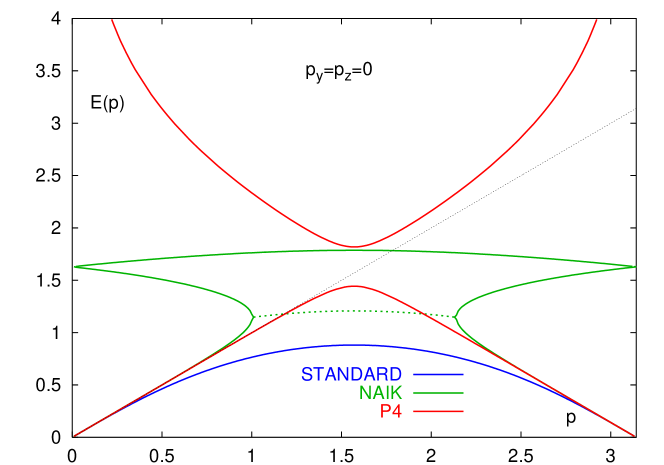
Figure 1: Dispersion relation $E=E(\vec{p})$ with $\vec{p}=(p,0,0)$ for the standard staggered fermion action (blue), the Naik-action (green) and the p4-action (red) compared to the continuum dispersion relation $E=p$. Solid and dashed lines denote real and complex poles of the propagator respectively.

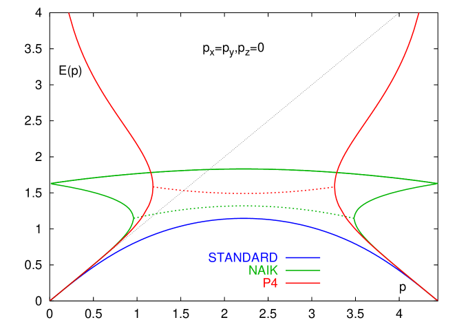
Figure 2: Dispersion relation $E=E(\vec{p})$ with $\vec{p}=(p/\sqrt{2},p/\sqrt{2},0)$ for the standard staggered fermion action (green), the Naik-action (blue) and the p4-action (red) compared to the continuum dispersion relation $E=p$. Solid and dashed lines denote real and complex poles of the propagator respectively.

The inverse free fermion propagator of the action 2 in momentum space takes the form

$${\Delta_{F}^{(0)}}^{-1}(p)={-i\sum_{\mu}\gamma_{\mu}h_{\mu}(p)+m\over\sum_{\rho}h_{\rho}^{2}(p)+m^{2}}={-i\sum_{\mu}\gamma_{\mu}h_{\mu}(p)+m\over D^{(0)}(p)+m^{2}}~{}~{},$$ (2.6)

where the functions $h_{\mu}(p)$ are given in appendix A.1 (Eq. A.2).
In order to obtain a rotational invariant free propagator we should achieve that $D^{(0)}(p)=\sum_{\mu}~{}h_{\mu}(p)h_{\mu}(p)$ is a function of ${\boldmath p}^{2}$ only. For the standard one-link propagator of the staggered fermion action this requirement for a rotational invariant propagator is violated at $\mathcal{O}(p^{4})$. Expanding $D^{(0)}(p)$, i.e. the trigonometric functions appearing in $h_{\mu}(p)$ (see appendix A.1), in orders of $p$ a further constraint to the coefficients $c^{(0)}_{i,j}$ can be determined such that the free propagator is rotational invariant up to order $p^{4}$, for details see appendix A.1. The constraint is

$$c^{(0)}_{1,0}+27~{}c^{(0)}_{3,0}+6~{}c^{(0)}_{1,2}=24~{}c^{(0)}_{1,2}~{}~{}.$$ (2.7)

Two simple choices which eliminate the bended or straight three link terms in 2, respectively, are to set either $c^{(0)}_{1,2}\equiv 0$ which yields the familiar Naik-action

$$c^{(0)}_{1,0}={9\over 16}~{}~{},~{}~{}c^{(0)}_{3,0}=-{1\over 48}~{}~{},$$ (2.8)

or to set $c^{(0)}_{3,0}\equiv 0$ which leads to

$$c^{(0)}_{1,0}={3\over 8}~{}~{},~{}~{}c^{(0)}_{1,2}={1\over 48}~{}~{},$$ (2.9)

which we will call the p4-action.
Since for the Naik-action the $\mathcal{O}(p^{4})$ terms are completely eliminated one gets even an $\mathcal{O}(a^{2})$ improvement, which seems quite accidental in this approach.

A first impression of how the improvement works is obtained by inspecting the dispersion relation $E=E(p_{x},p_{y},p_{z})$ resulting from the poles of the free propagator for massless fermions ${\Delta_{F}^{(0)}}^{-1}$, which are solutions of $D^{(0)}(iE,\vec{p})=0$. Figures 1 and 2 show the dispersion relations for on-axis momenta $\vec{p}=(p,0,0)$ and momenta on the planar diagonal $\vec{p}=(p/\sqrt{2},p/\sqrt{2},0)$ respectively for the standard fermion action, the Naik-action and the p4-action in comparison to the continuum relation $E(p)=p$. In case of the Naik-action for on-axis momenta as in case of Naik- and p4-action for planar diagonal momenta there are also complex poles of the propagator. The real part of these poles is plotted as thin line for distinction to the real poles. In the continuum limit $a\rightarrow 0$ only the branch in the lower left corner of the $E$-$p$ plane survives as $E=E_{\rm cont}\cdot a$ and $p=p_{\rm cont}\cdot a$. However, the finite cut-off $a$ leads to deviations from the continuum dispersion relation on finite lattices. But the plots indicate that the dispersion relations for the improved actions are close to the continuum for a much larger range of momenta compared to the standard action. In particular the dispersion relation of the p4-action is close to the continuum relation in nearly half the Brillouin zone for on-axis momenta. As will be discussed in section 3 this leads to a strong reduction of the cut-off dependence in the ideal gas ($g\rightarrow 0$) limit.

2.2 Improvement of rotational symmetry at ${\cal O}(g^{2})$

In order to reduce the violation of rotational symmetry also at ${\cal O}(g^{2})$ we again chose to look at the fermion propagator, as it is the most fundamental observable in the calculation of loop corrections to thermodynamic observables.
Expanding the link variables $U_{\mu}(x)=\exp(igA_{\mu}(x))$ one finds an expansion of the action in powers of g,

$$S=S^{(0)}+gS^{(1)}+g^{2}S^{(2)}+g^{2}\tilde{S}^{(0)}+\mathcal{O}(g^{3})~{}~{}.$$ (2.10)

Now expanding $e^{-S}$ one gets the following contributions to the fermion propagator in momentum space up to ${\cal O}(g^{2})$ :

$$\delta_{p,q}\cdot{{\Delta_{F}^{(2)}}^{-1}(p)}^{ab}_{\alpha\beta} = \left\langle\bar{\psi}_{\alpha}^{a}(q)\psi_{\beta}^{b}(p)\right\rangle$$

$$= \left\langle\bar{\psi}_{\alpha}^{a}(q)\psi_{\beta}^{b}(p)\right\rangle_{0}+g^{2}\Bigg{[}{1\over 2}\left\langle\bar{\psi}_{\alpha}^{a}(q)\psi_{\beta}^{b}(p)\left(S_{F}^{(1)}\right)^{2}\right\rangle_{0,c}$$

$$-\left\langle\bar{\psi}_{\alpha}^{a}(q)\psi_{\beta}^{b}(p)S_{F}^{(2)}\right\rangle_{0,c}-\left\langle\bar{\psi}_{\alpha}^{a}(q)\psi_{\beta}^{b}(p)\tilde{S}_{F}^{(0)}\right\rangle_{0,c}\Bigg{]}~{}~{},$$

where the subscripts indicate that the expectation values are taken with respect to the free action and that only connected parts are taken into account.

$$\left\langle\mathcal{O}\right\rangle_{0}\equiv{1\over Z_{0}}\int~{}\left[DU\right]\left[D\bar{\psi}D\psi\right]~{}\mathcal{O}~{}e^{-S^{(0)}} Z_{0}\equiv\int~{}\left[DU\right]\left[D\bar{\psi}D\psi\right]e^{-S^{(0)}}~{}.$$ ,

$(S_{F}^{(1)})^{2}$ and $S_{F}^{(2)}$ are the self-energy terms arising from the parts independent of the 1-loop coefficients $c^{(2)}_{i,j}$, whereas $\tilde{S}_{F}^{(0)}$ denotes the part depending on these. We note that $S_{F}^{(0)}$ and $\tilde{S}_{F}^{(0)}$ are formally the same terms apart from an exchange of tree-level and 1-loop coefficients. The explicit form of these contributions are given in appendix A.1.
An integration over the fermion and gluon fields yields, for massless fermions,

$${{\Delta_{F}^{(2)}}^{-1}(p)}^{ab}_{\alpha\beta}=\left[{\Delta_{F}^{(0)}}^{-1}(p)\left[\sum_{\mu}~{}i\gamma_{\mu}\left(D^{(0)}_{\mu}(p)+g^{2}~{}\left(\Sigma_{\mu}(p)+D^{(2)}_{\mu}(p)\right)\right)\right]{\Delta_{F}^{(0)}}^{-1}(p)\right]_{\alpha\beta}^{ab}~{}~{},$$

with

$$D^{(0)}_{\mu}(p) = \mbox{\raisebox{-19.91692pt}{\psfig{width=113.81102pt}}~{}}~{}~{},$$

$$D^{(2)}_{\mu}(p) = \mbox{\raisebox{-19.91692pt}{\psfig{width=113.81102pt}}~{}}~{}~{},$$

$$\Sigma_{\mu}(p) = \mbox{\raisebox{-19.91692pt}{\psfig{width=113.81102pt}}~{}}+\mbox{\raisebox{-19.91692pt}{\psfig{width=113.81102pt}}~{}}~{}~{}.$$

The explicit results are given in appendix A.3. The self-energy term contains, besides the usual continuum contribution $(S_{F}^{(1)})^{2}$, also a 1-loop term , $S_{F}^{(2)}$, which is a pure lattice artifact. The $D^{(2)}$ term, which arises from the non-zero 1-loop coefficients $c^{(2)}_{i,j}$, acts like a counter-term in the sense that it ought to adjust the 1-loop contributions, although it does not remove any divergence.
To achieve a rotational invariant fermion propagator to $\mathcal{O}(g^{2})$ we consider the denominator of ${\Delta_{F}^{(2)}}^{-1}(p)$, which can be written as

$$\mathcal{D}(p) \equiv \sum_{\mu}\left(D^{(0)}_{\mu}(p)+g^{2}~{}\left(\Sigma_{\mu}(p)+D^{(2)}_{\mu}(p)\right)\right)^{2}$$

$$= \sum_{\mu}D^{(0)}_{\mu}(p)D^{(0)}_{\mu}(p)+2g^{2}\sum_{\mu}D^{(0)}_{\mu}(p)\left(\Sigma_{\mu}(p)+D^{(2)}_{\mu}(p)\right)+\mathcal{O}(g^{4})~{}~{},$$

and demand that $\mathcal{D}$ should be a function of $p^{2}$ only, analogous to the tree level case discussed in section 2.1. By this demand one obtains constraints for the 1-loop coefficients $c^{(2)}_{i,j}$ analogous to the approach in the previous section. But in contrast to the tree level case a straight forward expansion in powers of $p$ is not possible due to the logarithmic divergence in the contributions arising from $(S_{F}^{(1)})^{2}$.
Alternatively we consider on-axis and off-axis momenta having the same magnitude, $p_{1}=(\tilde{p},0,0,0)$ and $p_{2}=(\tilde{p}/\sqrt{2},\tilde{p}/\sqrt{2},0,0)$, and then determine the coefficients by solving the equation

$$\mathcal{D}(p_{1})=\mathcal{D}(p_{2})$$ (2.11)

for small momenta $\tilde{p}$.
In general $\mathcal{D}(p)$ depends also on the fat-link-weight $\omega$. But since the fat-link-weight has a negligible effect on thermodynamics, as it will turn out in the next section, where we look at the free energy density at $\mathcal{O}(g^{2})$, we fix the value of the fat-link-weight to $\omega$=0 for this calculation. The restriction to one or the other 3-link term in the action together with the constraint 2.4 leaves only one free 1-loop parameter, which can be determined as solution of equation 2.11.

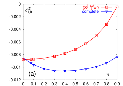
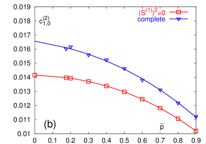
Figure 3: Solution of the equation 2.11 with complete contributions (blue) and without $(S_{F}^{(1)})^{2}$ contribution (red) for (a) the Naik-action and (b) the p4-action. Lines in case of the complete contributions are extrapolated by a polynomial fit.

The $\tilde{S}^{(0)}$ term is a simple function of $p$. In the different parts of the $S_{F}^{(2)}$ contribution the $p$ dependence can be factored out of the gluonic integrals. Thus, they can be computed once for all values of $p$. In appendix A.3 we show that only three distinct gluonic integrals appear in the $S_{F}^{(2)}$ contributions. These gluon-integrals have been calculated to high accuracy using Gauss-Legendre integration.
In principle one can expand these contributions in powers of $p$ as in the previous section, but in contrast to that the $(S_{F}^{(1)})^{2}$ contribution can not be expanded due to a logarithmic divergence in the $p\rightarrow 0$ limit. The gluon-loops have to be calculated for each of the momenta $\tilde{p}$ separately, since there is no factorization in gluonic and fermionic parts. The mentioned divergence causes also numerical difficulties for small fermion momenta $p$, where the pole of the inner gluon line, which is at $p-k=0$, runs into the pole of the gluon propagator at $k=0$. Therefore some care has to be taken to get reliable results. In practice this problem prohibits to perform our numerical integrations at arbitrary small $\tilde{p}$.

Solutions of the equation 2.11 are plotted in Figure 3 for the Naik-action and the p4-action as function of the momentum $\tilde{p}$. The squares are solutions for $c_{1,1}^{(2)}$, one obtains including only the $D^{(2)}$ term and the $S_{F}^{(2)}$ part of $\Sigma$, i.e. setting $(S_{F}^{(1)})^{2}$ to zero. Since the $p$ dependence of these parts is known explicitely we get precise results down to very small momenta. The triangles represent the solutions including all contributions. The scattering of points at small $\tilde{p}$ is due to the numerical difficulties in this regime for the $(S_{F}^{(1)})^{2}$ part. In the Naik case we obtain stable results for $\tilde{p}\geq 0.1$, whereas in the p4 case the results are trustable only for $\tilde{p}\geq 0.3$. In these regimes we have increased the number of Gaussian points until the values became stable, i.e. up to 320 Gaussian points in each direction for the small momenta.
These plots indicate that the main contribution to the violation of rotational symmetry originates from the $S_{F}^{(2)}$ part of the self-energy term which is quite reasonable since this term is a pure lattice artifact.

Using a polynomial fit we get the extrapolated values of the coefficients:

Naik-action	:	$c^{(2)}_{1,0}$	=	$-0.0085$	,	$c^{(2)}_{3,0}$	=	$0.00283$
p4-action	:	$c^{(2)}_{1,0}$	=	$0.0165$	,	$c^{(2)}_{1,2}$	=	$-0.00275$

It is remarkable that these coefficients indicate an over-improvement using the tree-level improvement at finite $g$, as the tree-level coefficients are corrected towards the standard staggered action.

3 Free energy in 1-loop perturbation theory

Thermodynamic observables show large cut-off dependencies in finite temperature lattice simulations. A suitable quantity to study the influence of finite cut-off effects on thermodynamic observables is the perturbative high temperature limit which is known from continuum perturbation theory up to order $g^{2}$ for a long time [10]. The free energy density for $n_{f}$ flavours of massless quarks and the $SU(N_{c})$ colour group is

$$f_{\rm cont} \equiv f^{(0)}_{{\rm cont},G}+f^{(0)}_{{\rm cont},F}+g^{2}\left(f^{(2)}_{{\rm cont},G}+f^{(2)}_{{\rm cont},F}\right)+{\cal O}(g^{3})~{}~{},{\rm where}$$

$$f^{(0)}_{{\rm cont},G}/T^{4} = -{1\over 45}\pi^{2}\left(N_{c}^{2}-1\right)~{}~{},$$

$$f^{(2)}_{{\rm cont},G}/T^{4} = {1\over 144}g^{2}\left(N_{c}^{2}-1\right)N_{c}~{}~{},$$

$$f^{(0)}_{{\rm cont},F}/T^{4} = -n_{f}{7\over 180}\pi^{2}N_{c}~{}~{},$$

$$f^{(2)}_{{\rm cont},F}/T^{4} = n_{f}{5\over 576}\left(N_{c}^{2}-1\right)~{}~{}.$$ (3.1)

Up to this order the thermodynamic relation $\epsilon=3p=-3f$ holds, where $\epsilon$ is the energy density, $p$ is the pressure and $f$ is the free energy density.
On lattices with temporal extension $N_{\tau}$ large ${\cal O}(1/N_{\tau}^{2})$, i.e. $\mathcal{O}((aT)^{2})$, deviations from 3.1 are found in the gluonic contribution for the standard plaquette action as well as in the fermionic part for the standard Kogut-Susskind action.
Tree level improved gauge actions reduce these cut-off effects in the leading order perturbative ideal gas limit. It has been shown that the improvement persists at finite temperatures well below those at which the ideal gas limit is approached [2]. In the fermionic sector thermodynamic observables show even larger deviations from the continuum Stefan-Boltzmann limit using the standard staggered fermion formulation [6]. By construction the Naik-action also reduces these deviations in the fermionic contributions to the energy density $\epsilon$ in leading order.
At 1-loop order it is known that the standard staggered action also leads to large cut-off dependent deviations in the energy density $\epsilon$ [8]. We will analyze in the following in how far these are reduced for the improved actions constructed in the previous section.

We calculate the fermionic contribution to the free energy density $f_{F}$ in lattice perturbation theory up to order $g^{2}$ for various fermion actions introduced in the previous section including the 1-loop improved actions and fat-link improvement. Only at this order will the influence of fat-link improvement, 1-loop coefficients and also the chosen gauge-action show up.
Since we are dealing with naive fermions the number of flavours is $n_{f}=16$. Up to 1-loop order lattice perturbation theory is equivalent for naive and staggered fermions and the correct $n_{f}$ dependence which only is a multiplicative factor at this order, can easily be introduced at the end [12]. We always chose the bare mass $m=0$ to get comparable results.
The reason that we chose the free energy density $f$ to look at is that it is defined by a very simple relation, just the logarithm of the partition function, instead of a derivative of the logarithm of the partition in case of the energy density $\epsilon$:

$$e^{-{V\over T}f_{F}} \equiv Z=\int~{}\left[DU\right]\left[D\bar{\psi}D\psi\right]e^{-S_{F}}$$ (3.2)

$$= Z_{0}\Bigg{\{}1-g^{2}\left[\left\langle S_{F}^{(2)}\right\rangle_{0}-{1\over 2}\left\langle\left(S_{F}^{(1)}\right)^{2}\right\rangle_{0}+\left\langle\tilde{S}_{F}^{(0)}\right\rangle_{0}\right]+\mathcal{O}(g^{3})\Bigg{\}}~{}~{}.$$

Here again we expanded the fermion action in powers of $g$. The subscript zero is defined as in the previous section and pure gluonic contributions are neglected also. Taking the logarithm of 3.2 one finds:

$$f_{F} = f^{(0)}_{F}+g^{2}f^{(2)}_{F}+\mathcal{O}(g^{3})$$ (3.3)

$$= f^{(0)}_{F}+g^{2}{T\over V}\left[\left\langle S_{F}^{(2)}\right\rangle_{0}-{1\over 2}\left\langle\left(S_{F}^{(1)}\right)^{2}\right\rangle_{0}+\left\langle\tilde{S}_{F}^{(0)}\right\rangle_{0}\right]+\mathcal{O}(g^{3})~{}.$$

Explicit expressions for the expansion coefficients are given in appendix A.4. The various contributions correspond to the following diagrams:
$\displaystyle f^{(0)}_{F}$ $\displaystyle=$ $\displaystyle\mbox{\raisebox{-17.07182pt}{\psfig{width=42.67912pt}}~{}}~{}~{}~{},$ $\displaystyle\left\langle\left(S_{F}^{(1)}\right)^{2}\right\rangle_{0}$ $\displaystyle=$ $\displaystyle\mbox{\raisebox{-36.98866pt}{\psfig{height=85.35826pt}}~{}}~{},$ $\displaystyle\left\langle\tilde{S}_{F}^{(0)}\right\rangle_{0}$ $\displaystyle=$ $\displaystyle\mbox{\raisebox{-17.07182pt}{\psfig{width=42.67912pt}}~{}}~{},$ $\displaystyle\left\langle S_{F}^{(2)}\right\rangle_{0}$ $\displaystyle=$ $\displaystyle\mbox{\raisebox{-36.98866pt}{\psfig{height=85.35826pt}}~{}}~{}.$

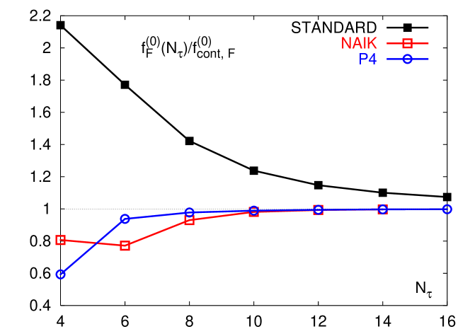
Figure 4: Fermionic tree level contribution to the free energy density normalized to the fermionic continuum tree level contribution as function of temporal extension $N_{\tau}$ for standard Kogut-Susskind action (black), Naik-action (red) and p4-action (blue).

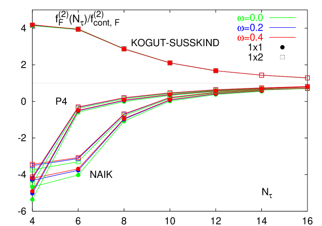
Figure 5: Fermionic 1-loop contribution to the free energy density normalized to the fermionic continuum 1-loop contribution as function of temporal extension $N_{\tau}$ for various fermion actions. Different colours represent the value of the fat-link parameter $\omega=0.0,~{}0.2,~{}0.4$. Circles denote the use of the standard gluon action, open squares the use of the 1$\times$2 gluon action. In the Naik- and p4-action only tree-level coefficients are included, i.e. $c_{i,j}^{(2)}\equiv 0$. The values for $N_{\tau}>8$ are extrapolated.

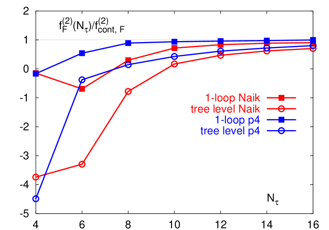
Figure 6: Fermionic 1-loop contribution to the free energy density normalized to the fermionic continuum tree level contribution as function of temporal extension $N_{\tau}$ for the Naik-action (red) and the p4-action (blue) including only tree-level improvement, i.e. $c_{i,j}^{(2)}\equiv 0$, (open circles) and including also 1-loop improvement (squares). Always the 1$\times$2 gluon action is used. The values for $N_{\tau}>8$ are extrapolated.

Obviously there is a correspondence between these contributions and those to the fermion propagator discussed in the previous section. One gets the graphs just by connecting the incoming and outgoing fermion lines of the diagrams of the fermion propagator. The $\tilde{S}_{F}^{(0)}$ contribution includes the whole dependence on the 1-loop coefficients and does not contribute if these are ignored. The $S_{F}^{(2)}$ term again can be factorized in fermionic and gluonic loop integrals in contrast to the $(S_{F}^{(1)})^{2}$ term.
In order to extract the finite temperature contribution we calculated the difference of the free energy density on $N_{\sigma}^{3}\times N_{\tau}$ and $N_{\sigma}^{4}$ lattices. The spatial extension was set to infinity, $N_{\sigma}=\infty$. The loop integrals over spatial momenta were done using Gauss-Legendre integration. For the zero temperature contributions also the temporal momenta were integrated over with Gauss-Legendre integration, while for the finite temperature contributions the finite sums over temporal momenta were carried out explicitly.
The numerical effort to calculate the 2-loop integrals in particular for the $(S_{F}^{(1)})^{2}$ term is large and grows like $(\#$Gauss-points$)^{8}$, therefore the number of Gaussian points was at maximum 32 in each direction, which is a total number of about $10^{12}$ points. For small temporal extension $N_{\tau}\leq 8$ one finds a good convergence of the 2-loop contributions increasing the number of Gaussian points up to 32. For larger values of $N_{\tau}$, however, the limit is not reached with this maximum number of points. However, since the results show a clear $(\#$Gauss-points$)^{-4}$ behaviour they can be extrapolated to infinite number of Gaussian points also for $N_{\tau}>8$. Of course the uncertainty of the extrapolation grows with increasing $N_{\tau}$, but since our main interest lies in the deviations from continuum perturbation theory for small values of $N_{\tau}$ this does not affect our conclusions.

Figure 4 shows the deviations of the fermionic tree-level contributions to the free energy density from the Stefan-Boltzmann limit for the standard staggered fermion action, the Naik-action and the p4-action. The improved actions reduce the large cut-off dependent deviation of the standard action drastically from more than 20 at $N_{\tau}$=4 to about 20% in case of the Naik-action and about 40% in case of the p4-action. At $N_{\tau}$=6 and greater the improvement works even better. Here the deviations for the p4-action are below a few percent compared to nearly 80% for the standard action at $N_{\tau}$=6.
The results for the fermionic part of the free energy density at order $g^{2}$, $f^{(2)}$, normalized to the continuum order $g^{2}$ contribution, $f_{\rm cont}^{(2)}$, are plotted in Figures 5 and 6. Figure 5 shows the influence of fat-link improvement and the chosen gauge action for the considered tree-level improved and the standard staggered fermion actions, i.e. 1-loop coefficients are set to zero. For all actions large deviations from the continuum value are found at small values of $N_{\tau}$, although the p4-actions approach the continuum value most rapidly. The main differences are caused by the choice of tree-level coefficients of the fermion action rather than the gauge action or the fat-link parameter $\omega$. This is not unexpected, because fat-link improvement affects the infrared behaviour and reduces flavour symmetry breaking rather than the ultraviolet regime which is responsible for the high temperature behaviour. Further, improved gauge actions are designed to reduce cut-off distortions in the gluonic contributions, but they have shown to reduce flavour symmetry breaking also [13], which indicates rather an influence on infrared sensitive fermionic observables.

The influence of 1-loop improvement of Naik- and p4-action provided in the previous section on the high temperature behaviour at order $g^{2}$ is shown in Figure 6. Here in all cases the 1$\times$2 gauge action is used and the fat link parameter equals zero. The plot indicates a large reduction of cut-off effects at order $g^{2}$ for both types of 1-loop improved fermion actions compared to the corresponding tree-level action. Already at $N_{\tau}$=6 the deviations are reduced to less than 50% for the 1-loop p4-action and to about 140% for the 1-loop Naik-action, where the 1-loop contribution for the standard staggered action is about 4 times larger than the continuum 1-loop value.

As stated in the previous section, the 1-loop coefficients correct the tree-level coefficients towards the standard action in both cases, Naik- and p4-action. In correspondence to that we observe a change of the sign of $f_{F}^{(2)}$ comparing standard and tree-level improved actions, i.e. an “over-improvement” concerning the order $g^{2}$, which is reduced when including the 1-loop coefficients.

4 Conclusion

In this work we have presented a perturbative construction of staggered fermion actions with improved rotational symmetry of the fermion propagator at tree-level as well as in 1-loop order. In particular we considered tree-level and 1-loop improved versions of the Naik- and the p4-action both with and without additional fat-link improvement.
The tree-level improvement shows up in the dispersion relation which is close to the continuum relation in a much larger momentum range for the improved actions than for the standard action.
A perturbative calculation of the fermionic tree-level and 1-loop contributions to the free energy density $f$ has been performed to investigate the influence of improved rotational symmetry and fat-link improvement on the high temperature behaviour. At tree level as well as in 1-loop order the standard staggered action leads to large cut-off dependent deviations from the perturbative continuum value. We find a large reduction of these ultraviolet cut-off effects at tree-level for the tree-level improved actions. For example at $N_{\tau}=4$ the remaining cut-off effects are about a factor 10 smaller than the cut-off effects of the standard action.
Of course the coefficients of the $\mathcal{O}(a^{2})$ deviations depend on the observable. An earlier calculation of fermionic contributions to the energy density $\epsilon$ at tree-level has shown a reduction of cut-off distortions for the p4- and the Naik-action which is comparable to the results for the free energy density we present in this work although in case of the energy density one finds even smaller deviations for the p4-action of about 1% at $N_{\tau}$=4 [4].

Tree-level improvement, however, does not help at 1-loop order as expected. Our analysis showed that cut-off distortions are of comparable magnitude for the standard action as for the tree-level improved actions in the 1-loop contributions to the free energy density. It also turned out that fat-link improvement has a rather negligible influence on the high temperature behaviour, i.e. it neither reduces nor increases the cut-off effects significantly. This is not surprising since fat-link improvement was designed to affect the infrared rather than the ultraviolet behaviour.
Finally we find a large reduction of these ultraviolet cut-off effects at 1-loop order for the actions with improved rotational symmetry up to $\mathcal{O}(g^{2})$. Already at $N_{\tau}$=6 the deviations are reduced to less than half of the continuum 1-loop value for the 1-loop p4-action and to about $1.4$-times the continuum value for the 1-loop Naik-action, where the 1-loop contribution for the standard staggered action is about 4 times larger than the continuum 1-loop value.
Therefore the 1-loop improved p4-action in combination with fat-links is a particularly suitable candidate for finite temperature simulations in full QCD, combining the advantages of an improved high temperature behaviour up to 1-loop order with an improved flavour symmetry. And last but not least it retains the simplicity of the contributing local operators.

Acknowledgments   This work was partly supported by the TMR network Finite Temperature Phase Transitions in Particle Physics, EU contract no. ERBFMRX-CT97-0122. The work of U.M.H. was partly supported by DOE contracts DE-FG05-85ER250000 and DE-FG05-96ER40979, and he gratefully acknowledges support from the Zentrum für Interdisziplinäre Forschung, Universität Bielefeld.

Appendix A Appendix

We give here explicit expressions as well as some technical details of the perturbative calculations. It is organized as follows: In part A.1 we define the fundamental terms and functions we refer to in the following parts. Part A.2 and part A.3 contain some details of the determination of the tree-level and 1-loop coefficients respectively. In part A.4 we give the explicit results of the 1-loop calculation of the fermionic contribution to the free energy density.

A.1 General 1-loop results and definitions

For the trigonometric functions we use the short hand notation:

$$s_{\mu}(p) \equiv \sin(p_{\mu})~{}~{},$$

$$c_{\mu}(p) \equiv \cos(p_{\mu})~{}~{}.$$

The inverse gluon propagator of the 1$\times$2 action was calculated in [2]. For the standard plaquette action as for the 1$\times$2 action the propagator can be written as

$${\Delta_{G}}_{\mu,\nu}(k) = {D_{G}}_{\mu}(k)\delta_{\mu,\nu}-{E_{G}}_{\mu,\nu}(k)+\xi~{}g_{\mu}(k)g_{\nu}(k)~{},$$

$${D_{G}}_{\mu}(k) = 4~{}a_{1,1}~{}\sum_{\nu}s_{\nu}^{2}(k/2)-16~{}a_{1,2}~{}\sum_{\nu}s_{\nu}^{2}(k/2)\left(2-s_{\nu}^{2}(k/2)-s_{\mu}^{2}(k/2)\right)~{},$$

$${E_{G}}_{\mu,\nu}(k) = 4~{}a_{1,1}~{}s_{\mu}(k/2)s_{\nu}(k/2)$$

$$-16~{}a_{1,2}~{}s_{\mu}(k/2)s_{\nu}(k/2)\left(2-s_{\nu}^{2}(k/2)-s_{\mu}^{2}(k/2)\right)~{}~{},$$

with $a_{1,1}\equiv 1$, $a_{1,2}\equiv 0$ for the standard Wilson one-plaquette action and $a_{1,1}\equiv 5/3$, $a_{1,2}\equiv-1/12$ for the 1$\times$2 action. In both cases we choose the gauge fixing term $g_{\mu}(k)=2s_{\mu}(k/2)$ and Feynman gauge $\xi=1$.

The basis of our 1-loop calculations is an expansion of the fermion action in powers of the bare coupling $g$:

$$S_{F}=S_{F}^{(0)}+gS_{F}^{(1)}+g^{2}S_{F}^{(2)}+g^{2}\tilde{S}_{F}^{(0)}+\mathcal{O}(g^{3})~{}~{}.$$ (A.1)

To achieve that, we expand the exponential representation of the link variables $U_{\mu}(x)=\exp(igaA_{\mu}(x))$, with the gauge fields $A_{\mu}\equiv\sum_{b=1}^{N_{c}^{2}-1}A_{\mu}^{b}\lambda^{b}$ and normalization $2{\rm Tr~{}}\lambda^{a}\lambda^{b}=\delta_{ab}$ for the group generators $\lambda^{a}$. The lattice spacing is set to $a=1$. In momentum space we find then

$$S_{F}^{(0)} = i\int_{p}\bar{\psi}(p)\left\{\sum_{\mu}\gamma_{\mu}h_{\mu}(p)+m\right\}\psi(p)~{},$$

$$\tilde{S}_{F}^{(0)} = i{N_{c}^{2}-1\over 2N_{c}}\int_{p}\bar{\psi}(p)~{}\sum_{\mu}\gamma_{\mu}h^{(2)}_{\mu}(p)~{}\psi(p)~{},$$

$$S_{F}^{(1)} = i\int_{p}\int_{k}\bar{\psi}(p)~{}\sum_{\mu}\gamma_{\mu}\hat{S}^{(1)}_{\mu}(p,k)~{}\psi(p-k)~{},$$

$$S_{F}^{(2)} = -{i\over 2}\int_{p}\int_{k_{1}}\int_{k_{2}}\bar{\psi}(p)~{}\sum_{\mu}\gamma_{\mu}\hat{S}^{(2)}_{\mu}(p,k_{1},k_{2})~{}\psi(p-k_{1}-k_{2})~{},$$

where

$$\hat{S}^{(1)}_{\mu}(p,k) = \sum_{\rho}~{}K_{\mu;\rho}(p,k)~{}A_{\rho}(k)~{},$$

$$\hat{S}^{(2)}_{\mu}(p,k_{1},k_{2}) = \sum_{\rho,\sigma}~{}L_{\mu;\rho,\sigma}(p,k_{1},k_{2})~{}A_{\rho}(k_{1})A_{\sigma}(k_{2})~{}~{}.$$

Here we use the following definitions also referred to in appendices A.2 - A.4:

$$h_{\mu}(p) = 2~{}s_{\mu}(p)\Big{[}c_{1,0}^{(0)}+2~{}c_{1,2}^{(0)}\sum_{\nu\not=\mu}c_{\nu}(2p)\Big{]}+2~{}c_{3,0}^{(0)}s_{\mu}(3p)~{},$$ (A.2)

$$h^{(2)}_{\mu}(p) = 2~{}s_{\mu}(p)\Big{[}c_{1,0}^{(2)}+2~{}c_{1,2}^{(2)}\sum_{\nu\not=\mu}c_{\nu}(2p)\Big{]}+2~{}c_{3,0}^{(2)}s_{\mu}(3p)~{},$$

$$K_{\mu;\rho}(p,k) = c_{1,0}^{(0)}~{}\mathcal{A}^{\rm fat}_{\mu;\rho}(\omega;p,k)+c_{3,0}^{(0)}~{}\mathcal{A}^{(3,0)}_{\mu;\rho}(p,k)+c_{1,2}^{(0)}~{}\mathcal{A}^{(1,2)}_{\mu;\rho}(p,k)~{},$$

$$L_{\mu;\rho,\sigma}(p,k_{1},k_{2}) = c_{1,0}^{(0)}~{}\mathcal{B}^{\rm fat}_{\mu;\rho,\sigma}(\omega;p,k_{1},k_{2})+c_{3,0}^{(0)}~{}\mathcal{B}^{(3,0)}_{\mu;\rho,\sigma}(p,k_{1},k_{2})+c_{1,2}^{(0)}~{}\mathcal{B}^{(1,2)}_{\mu;\rho,\sigma}(p,k_{1},k_{2})~{},$$

where

$$\mathcal{A}^{\rm fat}_{\mu;\rho}(\omega;p,k) = 2~{}c_{\mu}(p-k/2)$$

$$\cdot\Bigg{[}\delta_{\mu,\rho}-{4\omega\over 1+6\omega}\Bigg{(}\delta_{\mu,\rho}\sum_{\nu\not=\mu}s_{\nu}^{2}(k/2)-(1-\delta_{\mu,\rho})~{}s_{\mu}(k/2)s_{\rho}(k/2)\Bigg{)}\Bigg{]}~{},$$

$$\mathcal{B}^{\rm fat}_{\mu;\rho,\sigma}(\omega;p,k_{1},k_{2}) = 2~{}s_{\mu}(p-k_{1}/2-k_{2}/2)$$

$$\cdot\Bigg{[}\delta_{\mu,\rho}\delta_{\mu,\sigma}-{4\omega\over 1+6\omega}\Bigg{(}\delta_{\mu,\rho}\delta_{\mu,\sigma}\sum_{\nu\not=\mu}s_{\nu}^{2}(k_{1}/2+k_{2}/2)$$

$$\qquad+2~{}(1-\delta_{\mu,\rho})~{}\delta_{\rho,\sigma}~{}s_{\mu}(k_{1}/2)s_{\mu}(k_{2}/2)c_{\rho}(k_{1}/2+k_{2}/2)$$

$$\qquad-\delta_{\mu,\rho}~{}(1-\delta_{\mu,\sigma})~{}\{s_{\mu}(k_{2}/2)-ic_{\mu}(k_{2}/2)\}~{}s_{\sigma}(k_{1}+k_{2}/2)$$

$$\qquad-\delta_{\mu,\sigma}~{}(1-\delta_{\mu,\rho})~{}\{s_{\mu}(k_{1}/2)+ic_{\mu}(k_{1}/2)\}~{}s_{\sigma}(k_{2}+k_{1}/2)\Bigg{)}\Bigg{]}~{},$$

$$\mathcal{A}^{(3,0)}_{\mu;\rho}(p,k) = 2~{}\delta_{\mu,\rho}~{}c_{\mu}(3p-3k/2)\left(3-4s_{\mu}^{2}(k/2)\right)~{},$$

$$\mathcal{B}^{(3,0)}_{\mu;\rho,\sigma}(p,k_{1},k_{2}) = 2~{}\delta_{\mu,\rho}~{}\delta_{\mu,\sigma}~{}s_{\mu}(3p-3k_{1}/2-3k_{2}/2)\left[9-4s_{\mu}^{2}(k_{1}/2+k_{2}/2)\right.$$

$$\qquad\qquad\qquad\left.-4s_{\mu}^{2}(k_{1}/2)-4s_{\mu}^{2}(k_{2}/2)-4s_{\mu}^{2}(k_{1}/2-k_{2}/2)\right]$$

$$\mathcal{A}^{(1,2)}_{\mu;\rho}(p,k) = 4~{}c_{\mu}(p-k/2)~{}\delta_{\mu,\rho}\sum_{\nu\not=\mu}c_{\nu}(2p-k)c_{\nu}(k)$$

$$-8~{}(1-\delta_{\mu,\rho})~{}s_{\mu}(p-k/2)c_{\mu}(k/2)s_{\rho}(2p-k)c_{\rho}(k/2)~{},$$

$$\mathcal{B}^{(1,2)}_{\mu;\rho,\sigma}(p,k_{1},k_{2}) = 4~{}s_{\mu}(p-k_{1}/2-k_{2}/2)$$

$$\cdot\Bigg{[}\delta_{\mu,\rho}~{}\delta_{\mu,\sigma}\sum_{\nu\not=\mu}c_{\nu}(k_{1}+k_{2})c_{\nu}(2p-k_{1}-k_{2})$$

$$+2~{}(1-\delta_{\mu,\rho})~{}\delta_{\rho,\sigma}~{}c_{\mu}(k_{1}/2+k_{2}/2)$$

$$\cdot\Big{(}c_{\rho}(2p-3k_{1}/2-k_{2}/2)+c_{\rho}(2p-k_{1}-k_{2})c_{\rho}(k_{1}/2+k_{2}/2)\Big{)}\Bigg{]}$$

$$+8~{}\delta_{\mu,\rho}~{}(1-\delta_{\mu,\sigma})c_{\rho}(p-k_{1}/2)c_{\sigma}(k_{2}/2)s_{\sigma}(2p-2k_{1}-k_{2})$$

$$+8~{}\delta_{\mu,\sigma}~{}(1-\delta_{\mu,\rho})c_{\sigma}(p-k_{1}-k_{2}/2)c_{\rho}(k_{1}/2)s_{\rho}(2p-k_{1})~{}.$$

The integral symbols with subscripts for fermion and gluon momenta, denoted by the letters $p$ and $k$ respectively, actually denote a sum over the momentum modes on finite $N_{\sigma}^{3}\times N_{\tau}$. They are defined as:

$$\int_{k} = {1\over N_{\sigma}^{3}N_{\tau}}\sum_{k}~{}~{}{\rm with}\left\{\begin{array}[]{l@{~,~}l}k_{\mu}={2\pi n_{\mu}\over N_{\sigma}}\hfil~{},~{}&-{1\over 2}N_{\sigma}\leq n_{\mu}\leq{1\over 2}N_{\sigma}-1,~{}\mu\not=4\\ k_{4}={2\pi n_{4}\over N_{\tau}}\hfil~{},~{}&-{1\over 2}N_{\tau}\leq n_{4}\leq{1\over 2}N_{\tau}-1\end{array}\right.,$$ (A.5)

$$\int_{p} = {1\over N_{\sigma}^{3}N_{\tau}}\sum_{p}~{}~{}{\rm with}\left\{\begin{array}[]{l@{~,~}l}p_{\mu}={2\pi n_{\mu}\over N_{\sigma}}\hfil~{},~{}&0\leq n_{\mu}\leq N_{\sigma}-1,~{}\mu\not=4\\ p_{4}={\pi\left(2n_{4}+1\right)\over N_{\tau}}\hfil~{},~{}&0\leq n_{4}\leq N_{\tau}-1\end{array}\right..$$ (A.8)

The shift of temporal fermion momentum modes, $p_{4}$, represents antiperiodic boundary conditions in the time direction. As we consider the infinite volume limit the sum becomes an integral over the Brillouin zone, $1/N_{\sigma}\sum_{l_{i}}\rightarrow 1/(2\pi)\int_{-\pi}^{\pi}{\rm d}l_{i}$, $i=1,2,3$, for both fermionic and gluonic momenta, $l=p,k$. The same holds for the time direction in the zero temperature contributions.

The path integrals over the fermionic and gluonic fields are evaluated using the identities

$$\left\langle A^{a}_{\mu}(k)A^{b}_{\nu}(-l)\right\rangle_{0} = {N_{c}^{2}-1\over 2N_{c}}~{}{\Delta^{-1}_{G}}_{\mu,\nu}(k)~{}\delta_{k,l}~{}\delta^{a,b}~{}~{},$$

$$\left\langle\bar{\psi}_{\alpha}^{a}(p)\psi^{b}_{\beta}(q)\right\rangle_{0} = {\left(i\sum_{\mu}\gamma_{\mu}h_{\mu}(p)-m\right)_{\alpha,\beta}\over s_{F}(p)}~{}\delta_{p,q}~{}\delta^{a,b}~{}~{},$$

with

$$s_{F}(p) = \sum_{\mu}h_{\mu}^{2}(p)+m^{2}~{}~{}.$$

A.2 Tree level coefficients for improved rotational symmetry

An expansion of the free inverse fermion propagator up to order $p^{4}$ yields

$$D^{(0)}(p)=\sum_{\mu}h_{\mu}(p)h_{\mu}(p)=\sum_{\mu}Ap_{\mu}^{2}A\left(A+2B_{1}p_{\mu}^{2}+2B_{2}\sum_{\nu\not=\mu}p_{\nu}^{2}\right)+\mathcal{O}(p^{6})~{}~{},$$

with coefficients

$$A = 2c^{(0)}_{1,0}+12c^{(0)}_{1,2}+6c^{(0)}_{3,0}~{}~{},$$

$$B_{1} = -{1\over 3}c^{(0)}_{1,0}-2c^{(0)}_{1,2}-9c^{(0)}_{3,0}~{}~{},$$

$$B_{2} = -8c^{(0)}_{1,2}~{}~{}.$$

Obviously the condition $B_{1}=B_{2}$ has to be satisfied to achieve rotational symmetry up to order $p^{4}$, which leads to the constraint

$$c^{(0)}_{1,0}+27~{}c^{(0)}_{3,0}+6~{}c^{(0)}_{1,2} = 24~{}c^{(0)}_{1,2}~{}~{}.$$

The expansion shows that setting $c^{(0)}_{1,2}\equiv 0$, i.e. the Naik-action, leads to vanishing $\mathcal{O}(p^{4})$ coefficients $B_{1}=B_{2}\equiv 0$, which corresponds even to an $\mathcal{O}(a^{2})$ improvement.

A.3 Improved rotational symmetry at $\mathcal{O}(g^{2})$

The explicite expressions for the $\mathcal{O}(g^{2})$ contributions to the fermion propagator are:

$$D^{(0)}_{\mu}(p) = -h_{\mu}(p)~{},$$

$$D^{(2)}_{\mu}(p) = -{N_{c}^{2}-1\over 2N_{c}}h^{(2)}_{\mu}(p)~{},$$

$$\Sigma_{\mu}(p) = \mathcal{K}_{\mu}(p)+\mathcal{L}_{\mu}(p)~{},$$

$$\mathcal{K}_{\mu}(p) = {N_{c}^{2}-1\over 2N_{c}}\int_{k}{1\over s_{F}(p-k)}\sum_{\nu}\sum_{\rho,\bar{\rho}}\bigg{[}h_{\mu}(p-k)K_{\nu;\rho}(p,k)K_{\nu;\bar{\rho}}(p-k,-k)$$

$$\qquad\qquad\qquad\qquad-2h_{\nu}(p-k)K_{\mu;\rho}(p,k)K_{\nu;\bar{\rho}}(p-k,-k)\bigg{]}{\Delta_{G}^{-1}}_{\rho,\bar{\rho}}(k)~{},$$

$$\mathcal{L}_{\mu}(p) = -{N_{c}^{2}-1\over 4N_{c}}\int_{k}\sum_{\rho,\bar{\rho}}L_{\mu;\rho,\bar{\rho}}(p,k,-k){\Delta_{G}^{-1}}_{\rho,\bar{\rho}}(k)~{}.$$

For $\mathcal{L}_{\mu}(p)$ which originates from the $S^{(2)}_{F}$ term the $p$ dependence can be factored out. To achieve this one has to express the trigonometrical functions of sums of $p$ and $k$ as sums of factorized ones. Then taking into account that ${\Delta_{G}^{-1}}_{\mu,\mu}(k)$ is an even function of all $k$-directions and that ${\Delta_{G}^{-1}}_{\mu,\nu}(k)$ is an odd function of $k_{\mu}$ and $k_{\nu}$ and an even function of the remaining $k$-directions one finds that a lot of terms are odd functions in some $k$-direction and therefore vanish upon integration. The remaining terms, without using fat links, i.e. taking $\omega=0$, include only three gluonic integrals:

$$\mathcal{L}_{\mu}(p) = -{N_{c}^{2}-1\over 4N_{c}}\Bigg{\{}s_{\mu}(p)~{}c_{1,0}^{(0)}~{}2~{}\mathcal{I}_{1}+s_{\mu}(3p)~{}c_{3,0}^{(0)}~{}2~{}\mathcal{I}_{2}$$

$$\qquad\qquad~{}+s_{\mu}(p)\sum_{\nu\not=\mu}c_{\nu}(2p)~{}~{}c_{1,2}^{(0)}\left(4~{}\mathcal{I}_{1}+16~{}\mathcal{I}_{3}\right)\Bigg{\}}~{}~{},$$

where the gluonic integrals are defined as

$$\mathcal{I}_{1} \equiv \int_{k}{\Delta_{G}^{-1}}_{1,1}(k)~{}~{},$$

$$\mathcal{I}_{2} \equiv \int_{k}\left(9-8s_{1}^{2}(k/2)-4s_{1}^{2}(k)\right){\Delta_{G}^{-1}}_{1,1}(k)~{}~{},$$

$$\mathcal{I}_{3} \equiv \int_{k}\left(c_{2}^{2}(k/2){\Delta_{G}^{-1}}_{2,2}(k)-s_{1}(k/2)c_{2}(k/2)s_{2}(k){\Delta_{G}^{-1}}_{1,2}(k)\right)~{}~{}.$$

A calculation of these integrals to high accuracy using Gauss-Legendre integration gives

$$\mathcal{I}_{1} = 0.1282908~{}~{},$$

$$\mathcal{I}_{2} = 0.0752730~{}~{},$$

$$\mathcal{I}_{3} = 0.5074740~{}~{}.$$

A.4 Contributions to free energy density

The explicite expressions for the fermionic contributions to the free energy density up to $\mathcal{O}(g^{2})$ are:

$$f_{0} = -2N_{c}\int_{p}\ln\left[s_{F}(p)\right]~{},$$

$$\left\langle\left(S_{F}^{(1)}\right)^{2}\right\rangle_{0} = 2(N_{c}^{2}-1)\int_{p}\int_{k}{1\over s_{F}(p)s_{F}(p-k)}\sum_{\mu,\bar{\mu}}\Bigg{\{}$$

$$\left[\delta_{\mu,\bar{\mu}}\left(\sum_{\rho}h_{\rho}(p)h_{\rho}(p-k)+m^{2}\right)-2h_{\mu}(p)h_{\bar{\mu}}(p-k)\right]$$

$$\sum_{\rho,\bar{\rho}}K_{\mu;\rho}(p,k)K_{\bar{\mu};\bar{\rho}}(p-k,-k){\Delta_{G}^{-1}}_{\rho,\bar{\rho}}(k)\Bigg{\}}~{},$$

$$\left\langle S_{F}^{(2)}\right\rangle_{0} = (N_{c}^{2}-1)\int_{p}\int_{k}{1\over s_{F}(p)}\sum_{\mu}h_{\mu}(p)\sum_{\rho,\bar{\rho}}L_{\mu;\rho,\bar{\rho}}(p,k,-k){\Delta_{G}^{-1}}_{\rho,\bar{\rho}}(k)~{},$$

$$\left\langle\tilde{S}_{F}^{(0)}\right\rangle_{0} = -(N_{c}^{2}-1)\int_{p}\sum_{\mu}{h_{\mu}(p)h_{\mu}^{(2)}(p)\over s_{F}(p)}~{}.$$

In $\left\langle S_{F}^{(2)}\right\rangle_{0}$ the $k$ integration/sum can again be factored, similarly as for $\mathcal{L}_{\mu}(p)$ in A.3.

References

• [1] G. Boyd, J. Engels, F. Karsch, E. Laermann, C. Legeland, M. LΓΌtgemeier and B. Petersson, Phys. Rev. Lett. 75 (1995) 4169.
• [2] B. Beinlich, F. Karsch and E. Laermann, Nucl. Phys. B462 (1996) 415.
• [3] A. Papa, Nucl. Phys. B478 (1996) 335.
• [4] A. Peikert, B. Beinlich, A. Bicker, F. Karsch and E. Laermann, Nucl. Phys. B (Proc. Suppl.) 63A-C (1998) 895.
• [5] F. Karsch, Nucl. Phys. B (Proc. Suppl.) 60A (1998) 169.
• [6] J. Engels, R. Joswig, F. Karsch, E. Laermann, M. LΓΌtgemeier and B. Petersson, Phys. Lett. B396 (1997) 210.
• [7] Y. Luo, Phys.Rev. D57 (1998) 265.
• [8] U. Heller and F. Karsch, Nucl. Phys. B258 (1985) 29.
• [9] T. Blum, C. DeTar, S. Gottlieb, U. M. Heller, J. E. Hetrick, K. Rummukainen, R. L. Sugar, D. Toussaint, M. Wingate , Phys. Rev. D55 (1997) 1133.
• [10] J.I. Kapusta, Nucl. Phys. B148 (1979) 461;
O.K. Kalshnikov and V.V. Klimov, Phys. Lett. 88B (1979) 328.
• [11] P. Arnold and C. Zhai, Phys.Rev. D50 (1994) 7603.
• [12] H.S. Sharatchandra, H.J.Thun and P. Weisz, Nucl. Phys. B192 (1981) 205.
• [13] C. Bernard, T. Blum, T.A. DeGrand, C. DeTar, C. McNeile, S. Gottlieb, U.M. Heller, J. Hetrick, K. Rummukainen, B. Sugar and D. Toussaint, Phys. Rev. D58 (1998) 014503.