[

UCSD/PTH/98-36

HLRZ1998/62

The glueball spectrum from an anisotropic lattice study

Colin J. Morningstar

Dept. of Physics, University of California at San Diego, La Jolla, California 92093-0319

Mike Peardon

John von Neumann-Institut für Computing and DESY, Forschungszentrum Jülich, D-52425 Jülich, Germany
(January 7, 1999)

The spectrum of glueballs below 4 GeV in the SU(3) pure-gauge theory is investigated using Monte Carlo simulations of gluons on several anisotropic lattices with spatial grid separations ranging from 0.1 to 0.4 fm. Systematic errors from discretization and finite volume are studied, and the continuum spin quantum numbers are identified. Care is taken to distinguish single glueball states from two-glueball and torelon-pair states. Our determination of the spectrum significantly improves upon previous Wilson action calculations.

PACS number(s): 12.38.Gc, 11.15.Ha, 12.39.Mk

]

I Introduction

The gluon self-coupling in quantum chromodynamics (QCD) suggests the existence of glueballs, bound states of mainly gluons. Incontrovertible experimental evidence for their existence remains elusive, however. A primary reason for this is the difficulty in extracting the properties of glueballs from the QCD lagrangian. Investigating glueball physics requires an intimate knowledge of the confining QCD vacuum, and such knowledge cannot be obtained using standard perturbative techniques. Numerical simulations of the theory on a space-time lattice currently provide the most reliable means of studying glueballs. However, correlation functions of gluonic exitations are notoriously difficult quantities to measure in Monte-Carlo simulations, requiring large-scale computer resources when applying standard stochastic techniques. Recently, the use of spatially coarse, temporally fine lattices and improved actions was demonstrated to dramatically increase the efficiency of glueball simulations[1].

The objective in this paper is to apply the techniques of Ref. [1] to substantially improve our knowledge of the glueball spectrum in the pure SU(3) gauge theory. Detailed information on this spectrum is important for validating models of confined gluons and may help focus experimental searches for candidate glueball resonances. We also view this calculation as a necessary first step before attempting to include the effects of quarks. Note that unlike the quenched approximation for mesons and baryons, the pure glue theory is a physical quantum field theory with a unitary S-matrix. First, we perform six simulations for spatial lattice spacings ranging from 0.1 to 0.4 fm to determine the energies of the lowest-lying stationary states in all of the symmetry channels allowed on a cubic lattice. In many channels, we also determine the energies of the first-excited states. Our goal is then to extract the masses of as many low-lying glueballs as possible from the 141 measurements which were made. Since the spectrum of glue defined in a box with periodic boundary conditions includes not only single glueball states, but also states consisting of several glueballs and/or torelons (gluon excitations which wrap around the toroidal lattice), a means of identifying the single glueballs must be employed to prune away all of the other unwanted states. An additional small-volume simulation is done to assist in this identification and to study the systematic errors from finite volume. Finally, discretization errors are treated by extrapolating the energies to the continuum limit and determining the continuum spin quantum numbers. The end result is a nearly complete survey of the glueball spectrum in the pure gauge theory below 4 GeV. We find a total of thirteen glueballs; two other tentative candidates are also located. With the exception of the light glueballs in the $0^{++}$ sector, our results significantly improve upon those from previous studies[2, 3, 4] of the complete low-lying glueball spectrum.

This paper is organized as follows. The details of the simulations, including the construction of the glueball operators, the generation of the gauge-field configurations, the extraction of energies from Monte Carlo estimates of the correlation functions, and the lattice spacing determinations in terms of the hadronic scale $r_{0}$, are described in Sec. II. All of our energy estimates in terms of the inverse temporal lattice spacing are presented in this section. In Sec. III, the differentiation of single glueball states from two-glueball and torelon-pair states is discussed. Systematic errors from finite volume are studied in Sec. IV. The removal of lattice spacing errors, including the extrapolations to the continuum limit and the identification of the continuum spin quantum numbers, is described in Sec. V. We also discuss the problematical scalar states in this section and cite ongoing efforts to reduce their discretization errors. Sec. VI presents a discussion of the spectrum, and our findings are summarized with an outline of future work in the concluding Sec. VII.

II Simulation Details

Our glueball mass determinations rely on numerical simulations of gluons on a hypercubic Euclidean space-time lattice with spatial and temporal spacings $a_{s}$ and $a_{t}$, respectively. The gluons are described by the improved action $S_{I\!I}$ used in Ref. [1]. The couplings in the action depend on two parameters, $\beta$ and $\xi$, and are determined using a combination of (tree-level) perturbation theory and mean-field theory, implemented by renormalizing the spatial link variables $U_{j}(x)\rightarrow U_{j}(x)/u_{s}$, where $u_{s}$ is given by the fourth root of the average plaquette[5]. The temporal link variables are not renormalized. The lattice anisotropy $a_{s}/a_{t}$ is given by $\xi$ at tree-level in perturbation theory. This action is intended for use with $a_{t}\ll a_{s}$, has $O(a_{s}^{4},a_{t}^{2},\alpha_{s}a_{s}^{2})$ discretization errors, where $\alpha_{s}$ is the QCD coupling, and couples only nearest-neighbor time slices, ensuring the free-gluon propagator has no spurious modes. In all cases, glueball effective masses are seen to converge monotonically from above. This is a very desirable feature since it validates the use of variational techniques to minimize excited-state contributions to the glueball correlation functions. Such techniques are crucial for precise glueball mass extractions.

On a simple cubic lattice, zero-momentum stationary glue states are characterized by their transformation properties under the octahedral point group $O$, combined with parity and charge conjugation operations. $O$ has 24 elements (which are all proper rotations) that fall into five conjugacy classes; the single-valued irreducible representations are labeled $A_{1}$, $A_{2}$, $E$, $T_{1}$, and $T_{2}$, (Schönfliess notation[6]) and have dimensions 1, 1, 2, 3, and 3, respectively[7]. The inclusion of parity results in the symmetry group known as $O_{h}=O\otimes C_{i}$, where $C_{i}$ denotes the two-element group consisting of the identity operation and spatial inversion. The conventional labels for the irreducible representations of $O_{h}$ are obtained from those of $O$ by appending a subscript $g$ for representations corresponding to states which are even under parity and $u$ for odd parity representations. However, we shall use a slightly different notation. Instead of the subscripts $g$ and $u$, we use superscripts $+$ and $-$, respectively, to indicate the eigenvalue $P$ of parity. Glueball states are also eigenstates of charge conjugation. We denote the eigenvalue of charge-conjugation parity by $C$, as usual, and introduce an additional superscript in the representation labels. We refer to the full symmetry group of zero-momentum glueball states on a simple cubic lattice as $O_{h}^{C}$ or $O^{PC}$; the irreducible representations are labeled $A_{1}^{PC}$, $A_{2}^{PC}$, $E^{PC}$, $T_{1}^{PC}$, and $T_{2}^{PC}$. For convenience, we use $R$ when referring to these labels in general. Note that when we use one of these labels to identify a particular state, we refer to the lowest-lying zero-momentum state in the symmetry channel indicated by the representation label. The first-excited state in a particular symmetry channel will be denoted by the representation label with an asterisk.

The mass of a glueball $G$ having spin $J$, parity $P$, and charge-conjugation parity $C$ can be extracted from the large-$t$ behavior of a lattice-regulated correlation function $C(t)=\langle 0|\bar{\Phi}^{(R)}(t)\,\bar{\Phi}^{(R)}(0)|0\rangle$, where $R$ is any irreducible representation of $O_{h}^{C}$ occurring in the subduced representation $J^{PC}\!\downarrow\!O_{h}^{C}$, and $\bar{\Phi}^{(R)}(t)=\Phi^{(R)}(t)-\langle 0|\Phi^{(R)}(t)|0\rangle$ is a gauge-invariant, translationally-invariant, vacuum-subtracted, real operator capable of creating a glueball from the QCD vacuum $|0\rangle$. As the temporal separation $t$ becomes large, this correlator tends to a single decaying exponential $\lim_{t\rightarrow\infty}C(t)=Z\exp(-m_{G}t)$, where $m_{G}$ is the energy of the lowest-lying state which can be created by the operator $\bar{\Phi}^{(R)}(t)$. To determine $m_{G}$, the correlator $C(t)$ must be calculated for large enough $t$ such that it is well approximated by its asymptotic form. Unfortunately, stochastic fluctuations in $C(t)$ remain roughly constant with $t$ while the signal falls rapidly and hence, the use of a glueball operator for which $C(t)$ attains its asymptotic form as quickly as possible is crucial for reliably extracting $m_{G}$. The energies of excited states in representation $R$ can be obtained from the large-$t$ behavior of a matrix of correlation functions $C_{ij}(t)=\langle 0|\bar{\Phi}_{i}^{(R)}(t)\,\bar{\Phi}_{j}^{(R)}(0)|0\rangle$, where each of the glueball operators $\bar{\Phi}_{i}^{(R)}(t)$ transforms as $R$ under all symmetry operations. Again, it is very important to use operators for which the matrix elements $C_{ij}(t)$ attain their expected asymptotic forms for $t$ as small as possible.

Such operators can be constructed by exploiting link-smearing and variational techniques as previously described in Ref. [1]. For each irreducible representation $R$, glueball operators on a given time-slice are constructed in a sequence of three steps. First, a set of six smearing schemes are applied to the spatial link variables. Each scheme is a sequence of single-link and double-link mappings which depend on parameters $\lambda_{s}$ and $\lambda_{f}$, respectively. We use the same six schemes described in Ref. [1]. Secondly, a set of basic real operators $\phi^{(R)}_{\alpha}(t)$ is constructed using linear combinations of gauge-invariant, path-ordered products of the smeared link matrices about various closed spatial loops; each such linear combination is invariant under spatial translations and transforms according to the irreducible representation $R$. The loop-shapes employed in our calculation, shown in Fig. 1, are chosen for their ease of computation; all orientations of these operators can be computed very efficiently by first storing the untraced products of links around the twelve spatial plaquettes stemming from each site on a time-slice, then tracing the appropriate products of these objects. Both single and double windings around the paths are used; this allows us to double the number of raw operators with only a small increase in computational effort.

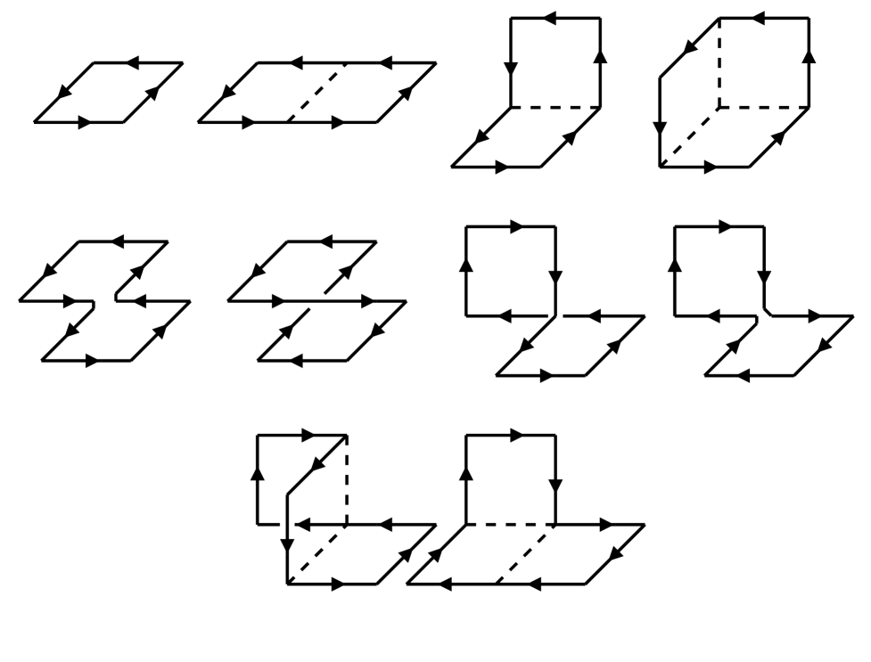
FIG. 1.: The Wilson loop shapes used in making the basic glueball operators.

For each symmetry channel except $A_{2}^{-+}$, four irreducible combinations are then chosen and applied to the smeared links from each of the six schemes, yielding a total of 24 basic operators in each channel. For the $A_{2}^{-+}$, only the last shape in Fig. 1 can be used and produces a total of 12 basic operators. Lastly, the glueball operators $\Phi^{(R)}(t)$ are formed from linear combinations of the basic operators, $\Phi^{(R)}(t)=\sum_{\alpha}v_{\alpha}^{(R)}\phi^{(R)}_{\alpha}(t)$, where the coefficients $v^{(R)}_{\alpha}$ are determined using the variational method. This involves first obtaining Monte Carlo estimates of the large correlation matrix

$$\tilde{C}_{\alpha\beta}(t)=\sum_{\tau}\langle 0|\bar{\phi}^{(R)}_{\alpha}(\tau\!+\!t)\>\bar{\phi}^{(R)}_{\beta}(\tau)|0\rangle,$$ (1)

where $\bar{\phi}^{(R)}_{\alpha}(t)=\phi^{(R)}_{\alpha}(t)-\langle 0|\phi^{(R)}_{\alpha}(t)|0\rangle$. In practise, this vacuum subtraction is only performed for the $A_{1}^{++}$ channel as the expectation value vanishes identically in all other sectors. The coefficients $v^{(R)}_{\alpha}$ are then chosen to minimize the effective mass

$$\tilde{m}(t_{D})=-\frac{1}{t_{D}}\ln\left[\frac{\sum_{\alpha\beta}v^{(R)}_{\alpha}v^{(R)}_{\beta}\ \tilde{C}_{\alpha\beta}(t_{D})}{\sum_{\alpha\beta}v^{(R)}_{\alpha}v^{(R)}_{\beta}\ \tilde{C}_{\alpha\beta}(0)}\right],$$ (2)

where the time separation for optimization is fixed to $t_{D}=1$. Other values of $t_{D}$ are used as consistency checks. Let ${\bf v}^{(R)}$ denote a column vector whose elements are the optimal values of the coefficients $v^{(R)}_{\alpha}$. This vector satisfies the eigenvalue equation

$$\tilde{C}(t_{D})\ {\bf v}^{(R)}=e^{-t_{D}\tilde{m}(t_{D})}\ \tilde{C}(0)\ {\bf v}^{(R)},$$ (3)

and the eigenvector ${\bf v}_{0}^{(R)}$ corresponding to the lowest effective mass $\tilde{m}_{0}(t_{D})$ yields the coefficients $v^{(R)}_{0\alpha}$ for the operator $\Phi^{(R)}_{0}(t)$ which, under ordinary circumstances, best overlaps the lowest-lying glueball $G_{0}$ in the channel of interest. A sequence of operators $\Phi^{(R)}_{1}(t),\Phi^{(R)}_{2}(t),\dots$ which predominantly overlap excited glueball states can also be constructed using the higher-mass eigenvectors of Eq. (3).

TABLE I.: The glueball simulation parameters. Values for the coupling $\beta$, input aspect ratio parameter $\xi$, the mean-link parameter $u_{s}^{4}$, the single-link smearing weight $\lambda_{s}$, the two-link smearing weight $\lambda_{f}$, and the lattice sizes are listed. Results for the hadronic scale $r_{0}$ in terms of the lattice spacing $a_{s}$ are also given. The approximate spatial lattice spacings $a_{s}$ are determined assuming $r_{0}^{-1}=410(20)$ MeV.

$\beta$	$\xi$	$u_{s}^{4}$	$\lambda_{s}$	$\lambda_{f}$	Lattice	$r_{0}/a_{s}$	$a_{s}/r_{0}$	$a_{s}$ (fm)
1.7	5	0.295	0.1	0.5	$6^{3}\times 30$	1.224(1)	0.8169(9)	0.39
1.9	5	0.328	0.1	0.5	$6^{3}\times 30$	1.375(2)	0.727(1)	0.35
2.2	5	0.378	0.1	0.5	$8^{3}\times 40$	1.761(2)	0.5680(5)	0.27
2.4	5	0.409	0.1	0.5	$8^{3}\times 40$	2.180(6)	0.459(1)	0.22
2.5	5	0.424	0.1	0.5	$10^{3}\times 50$	2.455(6)	0.407(1)	0.20
3.0	3	0.500	0.4	0.5	$15^{3}\times 45$	4.130(24)	0.2421(14)	0.12

Monte Carlo estimates of the correlator matrix elements given in Eq. (1) were obtained for all 20 irreducible representations in five simulations using an input aspect ratio parameter $\xi=5$. The values for the coupling $\beta$, mean-link parameter $u_{s}$, smearing weights $\lambda_{s}$ and $\lambda_{f}$, and the lattice sizes used in these runs are listed in Table I. An additional run at a smaller lattice spacing ($\sim 0.12$ fm) and using $\xi=3$ was done for the $A_{1}^{++}$, $E^{++}$, and $T_{2}^{++}$ representations only. A smaller-$a_{s}$ measurement helped to obtain a reliable continuum-limit extrapolation for the troublesome $A_{1}^{++}$ state. The input parameters for this run are also given in Table I. All computations were carried out on DEC Alpha and Sun Ultrasparc workstations. Configuration ensembles were generated using Cabibbo-Marinari (CM) pseudo-heatbath and SU(2) subgroup over-relaxation (OR) methods. Link variables were updated in serial order on the lattice. Three compound sweeps were performed between measurements, where a compound sweep is one CM updating sweep followed by $n_{\rm OR}$ OR sweeps. The measurements were averaged into bins of $n_{\rm mb}$, and $n_{\rm bins}$ bins were obtained. For the $\beta=3.0$, $\xi=3$ run, $n_{\rm OR}=5$, $n_{\rm mb}=50$, and $n_{\rm bins}=80$. For the $\beta=2.5$, $\xi=5$ run, $n_{\rm OR}=5$, $n_{\rm mb}=20$, and $n_{\rm bins}=318$. For all of the other simulations, $n_{\rm OR}=3$, $n_{\rm mb}=100$, and $n_{\rm bins}=100$. Crude checks for residual autocorrelations were done by over-binning by factors of two and four; in all cases, statistical error estimates remained unchanged.

TABLE II.: Glue energy estimates in terms of $a_{t}^{-1}$ for the five $\xi=5$ simulations. The levels are labeled by the irreducible representations of the cubic point group under which their corresponding stationary states transform. First-excited states in a representation are indicated by an asterisk.

	$\beta=1.7$	$\beta=1.9$	$\beta=2.2$	$\beta=2.4$	$\beta=2.5$
$A_{1}^{++}$	0.578(5)	0.475(4)	0.362(3)	0.303(3)	0.288(4)
$A_{1}^{\ast++}$	1.19(2)	0.92(3)	0.697(6)	0.569(4)	0.511(7)
$A_{2}^{++}$	1.43(2)	1.27(3)	1.018(12)	0.824(8)	0.713(14)
$E^{++}$	0.924(8)	0.844(6)	0.667(4)	0.538(3)	0.472(4)
$E^{\ast++}$	1.29(2)	1.093(12)	0.878(7)	0.723(9)	0.652(8)
$T_{1}^{++}$	1.55(2)	1.32(2)	1.00(2)	0.834(4)	0.728(8)
$T_{1}^{\ast++}$	1.73(3)	1.52(2)	1.23(4)	0.909(15)	0.823(13)
$T_{2}^{++}$	1.103(8)	0.918(7)	0.686(4)	0.542(2)	0.477(3)
$T_{2}^{\ast++}$	1.41(2)	1.228(12)	0.938(5)	0.730(8)	0.660(6)
$A_{1}^{-+}$	1.31(2)	1.06(5)	0.756(14)	0.605(11)	0.522(7)
$A_{1}^{\ast-+}$	1.86(9)	1.47(4)	1.08(2)	0.836(9)	0.72(2)
$A_{2}^{-+}$	—–	1.63(5)	1.29(2)	1.036(12)	0.93(1)
$E^{-+}$	1.38(2)	1.167(14)	0.874(5)	0.698(4)	0.611(7)
$E^{\ast-+}$	1.85(5)	1.49(3)	1.085(9)	0.890(6)	0.782(13)
$T_{1}^{-+}$	1.56(2)	1.42(2)	1.155(9)	0.873(13)	0.82(1)
$T_{2}^{-+}$	1.297(14)	1.148(10)	0.882(5)	0.695(4)	0.619(3)
$T_{2}^{\ast-+}$	1.60(2)	1.39(2)	1.087(9)	0.880(5)	0.771(9)
$A_{1}^{+-}$	—–	1.67(5)	1.32(2)	1.062(14)	0.94(1)
$A_{2}^{+-}$	—–	1.29(2)	0.999(11)	0.796(7)	0.700(14)
$E^{+-}$	—–	1.52(3)	1.207(37)	0.929(8)	0.82(1)
$T_{1}^{+-}$	1.186(13)	1.053(8)	0.819(4)	0.652(5)	0.590(5)
$T_{1}^{\ast+-}$	1.55(3)	1.297(14)	1.025(8)	0.794(9)	0.73(2)
$T_{2}^{+-}$	—–	1.330(16)	0.983(17)	0.801(4)	0.701(7)
$T_{2}^{\ast+-}$	—–	1.45(2)	1.10(3)	0.929(15)	0.83(1)
$A_{1}^{--}$	1.83(7)	1.61(5)	1.354(20)	1.04(3)	0.98(1)
$A_{2}^{--}$	—–	1.65(6)	1.201(18)	0.96(3)	0.82(2)
$E^{--}$	1.59(3)	1.38(2)	1.094(11)	0.875(6)	0.78(1)
$T_{1}^{--}$	1.72(4)	1.46(2)	1.07(3)	0.877(5)	0.760(9)
$T_{2}^{--}$	1.63(3)	1.41(2)	1.114(8)	0.886(6)	0.77(1)

In the final analysis phase, the glue energies $m_{G}$ were extracted using a two-step procedure. First, the large correlation matrices in each channel were reduced to smaller $3\times 3$ matrices $C_{AB}(t)$ for $A,B=0,1,2$ using the variational coefficients of the three lowest mass eigenstates of Eq. (3):

$$C_{AB}(t)=\sum_{\tau}\langle 0|\bar{\Phi}_{A}^{(R)}(\tau\!+\!t)\ \bar{\Phi}^{(R)}_{B}(\tau)|0\rangle.$$ (4)

Secondly, the expected large-$t$ functional forms were fit to the elements of these optimized correlators. To obtain an estimate of the energy $m_{G_{0}}$ (in terms of $a_{t}^{-1}$) of the lowest-lying state in each channel, a single exponential was fit to the ground-state correlator $C_{00}(t)$ for $t=t_{\rm min},\dots,t_{\rm max}$:

$$C_{00}(t)=Z_{00}\left\{e^{-m_{G_{0}}t}+e^{-m_{G_{0}}(T-t)}\right\},$$ (5)

where $T$ was the temporal extent of the periodic lattice. To determine the energies $m_{G_{p}}$ of the excited states and another estimate of $m_{G_{0}}$, the $M\times M$ optimized correlator matrix was also fit for $t=t_{\rm min},\dots,t_{\rm max}$ using the form

$$C_{AB}(t)=\sum_{p=0}^{M-1}Z_{Ap}Z_{Bp}\left\{e^{-m_{G_{p}}t}+e^{-m_{G_{p}}(T-t)}\right\},$$ (6)

for $M=2,3$. Various fit regions $t_{\rm min}$ to $t_{\rm max}$ were used to check for consistency in the extracted values for the masses. Best-fit values were obtained using the correlated $\chi^{2}$ method. Error estimates were calculated using a $1024-$point bootstrap procedure; in all cases, error estimates were nearly symmetric about the central best-fit values and were thus averaged to simplify presentation. Our fits are far too numerous to list here; additional details are available from the authors upon request.

Our final estimates of the glue energies in terms of $a_{t}^{-1}$ for the $\xi=5$ simulations are presented in Table II; energy estimates from the $\xi=3$ run are listed in Table III. In order to convert these results into physical units, the lattice spacings $a_{t}$ must be determined for each simulation. The hadronic scale parameter $r_{0}$ [8] defined in terms of the force between static quarks by $[r^{2}dV(\vec{r})/dr]_{r=r_{0}}=1.65$, where $V(\vec{r})$ is the static-quark potential, is a useful quantity for this purpose. The values for $r_{0}$ in terms of $a_{s}$ corresponding to each glueball simulation were determined by measuring the static-quark potential in separate simulations. The results are listed in Table I. Further details concerning the calculation of $r_{0}/a_{s}$ are given in Ref. [1]. Note that in computing $r_{0}/a_{s}$, the input value $\xi$ was used for the aspect ratio $a_{s}/a_{t}$. The consequences of doing so are discussed in Sec. V A.

TABLE III.: Glue energy estimates in units of $a_{t}^{-1}$ from the $\beta=3.0$, $\xi=3$ simulation.

$A_{1}^{++}$	0.318(4)
$E^{++}$	0.476(3)
$T_{2}^{++}$	0.476(3)

III Glueball identification

The spectrum in a box with periodic boundary conditions includes not only single glueball states, but also states consisting of several glueballs and/or torelons (gluon excitations which wrap around the toroidal lattice). We expect that the operators used in our correlators will couple most strongly to the single glueball states, but we cannot be certain that mixings with the multi-glueball and torelon states will be negligible. Recall that the asymptotic behavior of the correlation function associated with an operator $\Phi(t)$ is dominated by the lowest-lying eigenstate which mixes with $\Phi$. If a multi-glueball or torelon state has a lower energy than the lightest glueball in a given symmetry channel, then the possibility exists that the energy we extract from the asymptotic decay of the correlator will be that of the multi-glueball or torelon state. Thus, a means of differentiating the single glueball states from all other states is required.

First, given mass estimates of the lowest-lying few glueballs, one can easily determine the approximate locations in a given symmetry channel of the two-glueball states having zero total momentum. If the simulation results in that channel lie significantly below the two-glueball energy estimates, one can almost certainly rule out a multi-glueball interpretation.

Secondly, one can study the manner in which each energy level changes as the lattice volume is varied. The energy of a single glueball state depends on the lattice volume in a markedly different way from that of a multi-glueball or torelon state.

A third possibility is to include additional operators in the correlation matrices which are expected to couple much more strongly with the two-glueball and torelon states. The construction of operators which best overlap the lowest-lying eigenstates of interest using the variational method then involves not only single glueball operators, but also the new two-glueball and torelon operators. The coefficients obtained from the variational optimization can be used to estimate the mixings of the additional operators with the low-lying eigenstates of interest. If the mixings of the additional two-glueball and torelon operators with an eigenstate are very small, a single glueball interpretation is assured; in such a case, the addition of the new operators does not affect the extracted energy. If the mixings are significant, the addition of the two-glueball/torelon operators will lower the extracted energy, ruling out a single glueball interpretation.

Ideally, it would be best to apply all three of these methods. However, for this initial scan of the glueball spectrum, we decided for reasons of simplicity to rely mainly on the first method. Having obtained the lowest-lying one or two states in each symmetry channel, we determined the approximate locations of the two-glueball and torelon states. Simulation results lying near or above these thresholds were then excluded from further consideration. In other words, we used the two-glueball and torelon thresholds as filters to remove possibly extraneous states. One additional simulation was done to study systematic errors from finite volume. This run also served to confirm the single glueball nature of the states lying well below the two-glueball/torelon thresholds. Note that the levels lying near or above these thresholds cannot be ruled out as single glueball states; rather, one can say only that the interpretation of such states requires additional information.

A Two-glueball states

In order to identify the genuine single glueball states, we first determined the approximate locations of the two-particle states using the mass estimates of the lightest few glueballs. In estimating these locations, we assumed that the energy of a two-glueball state was given by

$$E_{2G}\approx\sqrt{\vec{p}^{2}+m_{1}^{2}}+\sqrt{\vec{p}^{2}+m_{2}^{2}},$$ (7)

where $m_{1}$ is the rest mass of the glueball having momentum $\vec{p}$ and $m_{2}$ is the rest mass of the other glueball which has momentum $-\vec{p}$. Note that on a periodic lattice having $N_{s}$ sites in each of the three spatial directions, the allowed momenta are discrete $\vec{p}=2\pi(n_{x},n_{y},n_{z})/L$, where $L=a_{s}N_{s}$ and $n_{x}$, $n_{y}$, and $n_{z}$ are integers satisfying $-N_{s}/2<n_{j}\leq N_{s}/2$. The above energy estimates neglect all interactions between the two glueballs; this should not introduce serious error since we expect these interactions to be short-ranged, being mediated by scalar glueball exchange at large distances. Eq. (7) also assumes that the rest masses and dispersion relations of the propagating glueballs are unaffected by finite volume and finite lattice spacing errors. We have verified this assumption in the case of the scalar glueball for $n_{x}^{2}+n_{y}^{2}+n_{z}^{2}<9$ on an $8^{3}\times 40$ lattice at $\beta=2.4$ and $\xi=5$.

TABLE IV.: The little groups of $\vec{p}=2\pi(n_{x},n_{y},n_{z})/L$ on a simple cubic lattice with periodic boundary conditions. Note that $l,m,n\neq 0$ and $l\neq m$, $m\neq n$, and $l\neq n$.

$(n_{x},n_{y},n_{z})$	Little group
$(0,0,0)$	$O_{h}$
$(0,0,n)$	$C_{4v}$
$(0,n,n)$	$C_{2v}$
$(n,n,n)$	$C_{3v}$
$(0,m,n)$	$C_{s}$
$(m,m,n)$	$C_{s}$
$(l,m,n)$	$C_{1}$

To facilitate our discussion of the two-glueball states, we first point out some features of single, propagating glueballs in a finite box with periodic boundary conditions. Here, glueball states are characterized by their transformation properties under $O_{h}^{1C}$, the simple cubic crystallographic space group $O_{h}^{1}$ extended to include charge-conjugation. The group $O_{h}^{1}$ is isomorphic to the semi-direct product of the group of pure (discrete) translations and the group of pure (discrete) rotations and reflections about a given center. Thus, a propagating glueball state may be classified by its momentum $\vec{p}$ and by its transformation properties under the subgroup of $O_{h}^{1C}$ which leaves $\vec{p}$ invariant (the little group of $\vec{p}$). The little groups corresponding to various momentum orientations are listed in Table IV. Hence, the irreducible representations of the little group may be used to identify propagating glueball states. The little group varies with the momentum orientation. This means that the partitioning of the physical glueball states into the irreducible representations of the lattice symmetry groups differs depending on the momentum orientation. For example, consider the $2^{++}$ glueball. When at rest, three of the five polarizations of this glueball appear in the $T_{2}^{++}$ representation of $O_{h}^{C}$, the little group of $\vec{p}=(0,0,0)$, and two of its polarizations occur in the $E^{++}$ representation. When $\vec{p}=(0,0,p)$ for $p\neq 0$, the five polarizations of the $2^{++}$ glueball (which are no longer eigenstates of parity) split across the $A_{1}^{+}$, $B_{1}^{+}$, $B_{2}^{+}$, and $E^{+}$ representations of the little group $C_{4v}^{C}$.

We determined the lowest-lying two-glueball states in each symmetry channel by repeating the following sequence of steps for each allowed momentum vector $\vec{p}$ and each choice of two glueballs $G_{1}$ and $G_{2}$. For the moment, assume that $G_{1}$ and $G_{2}$ are distinguishable. Note that $G_{1}$ and $G_{2}$ refer to the irreducible representations of $O_{h}^{C}$, the little group for zero momentum. First, we identified the little group $L(\vec{p})$ of $\vec{p}$. Secondly, the characters $\chi^{(G_{1})}$ and $\chi^{(G_{2})}$ of the representations $G_{1}$ and $G_{2}$ were subduced into the little group, yielding the characters $\chi^{(G_{j})}\!\downarrow\!L(\vec{p})$, which were then decomposed into the irreducible representations $\mu$ of the little group: $\chi^{(G_{j})}\!\downarrow\!L(\vec{p})=\sum_{\mu}c^{(G_{j})}_{\mu}\chi^{(\mu)}$. Next, for each $\mu_{1}$ such that $c^{(G_{1})}_{\mu_{1}}\neq 0$ and each $\mu_{2}$ such that $c^{(G_{2})}_{\mu_{2}}\neq 0$, we formed the direct product $\chi^{(\mu_{1}\otimes\mu_{2})}$ to obtain the character corresponding to the two-glueball state. Since the total momentum of this two-glueball state is zero, it can be characterized by the irreducible representations of $O_{h}^{C}$. A representation of $O_{h}^{C}$ was formed by constructing a set of coset representatives and applying the method of induction, and the induced character $\chi^{(\mu_{1}\otimes\mu_{2})}\!\!\uparrow\!\!O_{h}^{C}$ was finally decomposed into the irreducible representations of $O_{h}^{C}$. When $G_{1}$ and $G_{2}$ were indistinguishable, the above procedure was modified to include Bose symmetrization.

This procedure was carried out using the rest energies obtained in the $\beta=2.5$, $\xi=5$ simulation. The lowest-lying two-glueball states in each symmetry channel are listed in Table V. These levels, along with all higher lying levels, are shown as dashed line segments in the shaded region in Fig. 2. Any energy lying well below the shaded region in this figure can be safely interpreted as a single glueball state (these are indicated by the black-outlined green-filled boxes). States lying slightly below (the orange boxes with no outlines) or above (the red boxes) the two-glueball thresholds must be regarded with caution. Again, we remind the reader that we cannot rule out a single glueball interpretation for these levels; additional information is needed to determine the nature of these states. Since it is not our intent in this paper to obtain such information, we exclude these levels from the spectrum of single glueball states for the time being.

TABLE V.: The lowest lying state consisting of two free glueballs in each symmetry channel for the $\beta=2.5$, $\xi=5$ simulation. Each state is comprised of a glueball having a momentum $\vec{p}=2\pi(n_{x},n_{y},n_{z})/L$, where $L=10a_{s}$, and another glueball having momentum $-\vec{p}$.

Channel	Glueballs	$(n_{x},n_{y},n_{z})$
$A_{1}^{++}$	$(A_{1}^{++},A_{1}^{++})$	(0, 0, 0)
$A_{2}^{++}$	$(A_{1}^{++},E^{++})$	(0, 0, 1)
$E^{++}$	$(A_{1}^{++},A_{1}^{++})$	(0, 0, 1)
$T_{1}^{++}$	$(A_{1}^{++},A_{1}^{++})$	(0, 1, 2)
$T_{2}^{++}$	$(A_{1}^{++},A_{1}^{++})$	(0, 1, 1)
$A_{1}^{-+}$	$(A_{1}^{-+},A_{1}^{++})$	(0, 0, 0)
$A_{2}^{-+}$	$(A_{1}^{++},T_{2}^{++})$	(0, 0, 1)
$E^{-+}$	$(A_{1}^{++},T_{2}^{++})$	(0, 0, 1)
$T_{1}^{-+}$	$(A_{1}^{++},E^{++})$	(0, 0, 1)
$T_{2}^{-+}$	$(A_{1}^{++},E^{++})$	(0, 0, 1)
$A_{1}^{+-}$	$(A_{1}^{++},T_{1}^{+-})$	(0, 1, 2)
$A_{2}^{+-}$	$(A_{1}^{++},T_{1}^{+-})$	(0, 1, 1)
$E^{+-}$	$(A_{1}^{++},T_{1}^{+-})$	(0, 1, 1)
$T_{1}^{+-}$	$(A_{1}^{++},T_{1}^{+-})$	(0, 0, 0)
$T_{2}^{+-}$	$(A_{1}^{++},T_{1}^{+-})$	(0, 0, 1)
$A_{1}^{--}$	$(A_{1}^{++},T_{1}^{+-})$	(0, 0, 1)
$A_{2}^{--}$	$(A_{1}^{++},T_{1}^{+-})$	(0, 1, 1)
$E^{--}$	$(A_{1}^{++},T_{1}^{+-})$	(0, 0, 1)
$T_{1}^{--}$	$(A_{1}^{++},T_{1}^{+-})$	(0, 0, 1)
$T_{2}^{--}$	$(A_{1}^{++},T_{1}^{+-})$	(0, 0, 1)

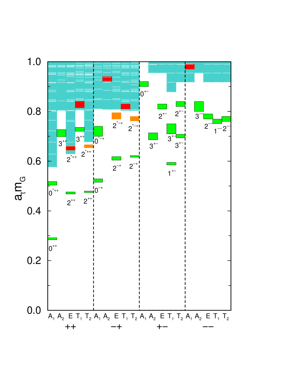
FIG. 2.: Comparison of the pure-glue spectrum obtained from the $\beta=2.5$, $\xi=5$ simulation to the approximate locations of the two glueball states. The boxes are the simulation results; the standard deviations in these mass estimates are indicated by the vertical heights of the boxes. The dotted line segments shown in the upper shaded region indicate the approximate locations of states consisting of two free glueballs having zero total momentum. All energies are in terms of $a_{t}^{-1}$. The representations of the cubic point group which label the states are indicated along the horizontal axis. The most likely $J^{PC}$ interpretations of the states are also shown.

B Torelon pairs

Torelons are gluonic excitations which wind around the periodic boundaries of the lattice. They may be classified according to their behavior under a set of discrete $Z_{3}$ symmetries of the SU(3) pure gauge theory. The gauge action is invariant under multiplication of every link in the $\mu$ direction ($\mu=0,1,2,3)$ at a given $\mu$ coordinate by the same member of $Z_{3}$, the center of SU(3). The torelon is an eigenstate of the transfer matrix which transforms nontrivially under such symmetry operations. For example, the spectrum of glue on a periodic lattice contains a torelon eigenstate which picks up a phase $\exp(2\pi i/3)$ and a state which picks up a phase $\exp(-2\pi i/3)$ under the multiplication of every link in the $x$-direction at a given $x$ coordinate by the center member $\exp(2\pi i/3)$. In fact, there are three such pairs of modes corresponding to the $x$, $y$, and $z$ directions. These torelons can also have a center-of-mass momentum in the two spatial directions transverse to their flux direction. For large $L$, a torelon at rest has an energy given approximately by $\sigma L$, where $\sigma$ is the string tension from the static-quark potential and $L$ is the spatial extent of the lattice. We have confirmed this in a simulation on an $8^{3}\times 24$ lattice at $\beta=2.4$, $\xi=3$. Hence, the torelon mass is strongly dependent on the volume of the lattice.

Our glueball operators, being closed Wilson loops which do not wrap around the lattice, are invariant under these center symmetry transformations. This means that the glueball operators cannot create a single torelon state, but the creation of torelon pairs of opposite center charge is possible. If the two torelons of opposite charge do not substantially interact, then the lowest energy of such a state is $2\sigma L$, which has the value 0.9 when placed on Fig. 2. This lies sufficiently high to discard from consideration, even for the $A_{1}^{+-}$ state since a state of two torelons of opposite center charge and total zero momentum must be symmetric under charge conjugation. Fortunately, a torelon pair can be easily detected in a finite-volume study since their energy depends strongly on $L$. An additional simulation was done to measure the changes in all energy levels as the lattice volume was reduced. The results of this simulation are presented in the next section. No energy reductions of sufficient magnitude were found to suggest that any of our states could be interpreted as a torelon pair.

IV Finite volume errors

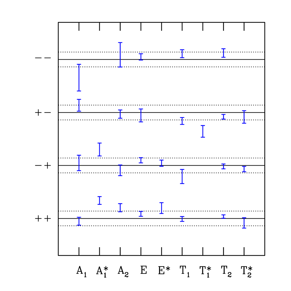
FIG. 3.: Finite-volume effects on the results of the $\beta=2.4$, $\xi=5$ simulation. Each point shows the fractional change $\delta_{G}=1-m_{G}^{S}/m_{G}$ in the energy of a stationary state $G$, where $m_{G}$ is the energy of $G$ as measured on an $8^{3}\times 40$ lattice, and $m_{G}^{S}$ is the energy of $G$ as measured on a smaller $6^{3}\times 40$ lattice. The state $G$ corresponding to a given point is specified by combining the representation label below the point along the horizontal axis with the $PC$ value shown to its left along the vertical axis. The solid lines indicate $\delta_{G}=0$, the dotted lines above the solid lines indicate $\delta_{G}=0.02$, and the dotted lines below the solid lines indicate $\delta_{G}=-0.02$.

An additional simulation was done to measure the systematic errors in our results from finite volume: a run at $\beta=2.4$, $\xi=5$ on a $6^{3}\times 40$ lattice. The original $8^{3}\times 40$ lattice has a spatial volume of (1.76 fm)³, assuming that $a_{s}\sim 0.22$ fm from $r_{0}^{-1}=410(20)$ MeV. The additional simulation measures the changes in the glueball masses as the volume is reduced from (1.76 fm)³ to (1.32 fm)³. The input parameters used in this small-volume run were the same as those used in the larger volume simulation.

Let $m_{G}$ denote the energy of a state $G$ on the original $8^{3}\times 40$ lattice, and $m_{G}^{S}$ denote the energy of $G$ as measured on the smaller $6^{3}\times 40$ lattice. The fractional change in the energy is defined by $\delta_{G}=1-m_{G}^{S}/m_{G}$. The results for these fractional changes are shown in Fig. 3. Each point shows the fractional change in the energy of a state $G$ specified by combining the representation label below the point on the horizontal axis with the $PC$ value shown to its left on the vertical axis. The solid lines indicate $\delta_{G}=0$, the dotted lines above the solid lines indicate $\delta_{G}=0.02$, and the dotted lines below the solid lines indicate $\delta_{G}=-0.02$. The largest effects from finite volume occur in the $A_{1}^{\ast++}$ and $T_{1}^{\ast+-}$ states. All other changes are statistically consistent with zero, indicating that systematic errors in these results from finite volume are negligible. These results confirm the single glueball nature of all of the states, with the exception of the $A_{1}^{\ast++}$, lying well below the two-glueball thresholds (the black-outlined green-filled boxes in Fig. 2). Although the change in the energy of the $A_{1}^{\ast++}$ is not very large, it is sufficient to warrant further study of this level. For this reason, we withhold judgment on whether or not this level is a single glueball. Note that most of the states lying near or above the two-glueball thresholds (the orange and red boxes in Fig. 2) show very little finite volume dependence, suggesting that these states might actually be long-lived glueball resonances. Further study would be required to resolve this issue.

V Lattice spacing errors

There are two aspects to the removal of systematic errors from finite lattice spacing: extrapolation of the results to the continuum limit $a_{s}\!\rightarrow\!0$, and the identification of the continuum spin quantum numbers. In this section, we first carry out the $a_{s}\!\rightarrow\!0$ extrapolations of the candidate single-glueball levels remaining after the analysis of Sec. III, then deduce their continuum spin content.

A Continuum limit extrapolations

The glueball mass estimates in terms of $a_{t}^{-1}$, listed in Table II, were combined with the determinations of the hadronic scale $r_{0}/a_{s}$ presented in Table I. The results are shown in Figs. 4-7. In these figures, the dimensionless products of $r_{0}$ and the glueball mass estimates are shown as functions of $(a_{s}/r_{0})^{2}$. The solid symbols indicate the results from the $\xi=5$ simulations. The open symbols appearing to the right of the vertical dashed lines indicate results from the $\beta=3.0$, $\xi=3$ run, as well as $\xi=3$ results for the $A_{1}^{++}$ and $A_{1}^{\ast++}$ channels previously obtained in Ref. [1]. To remove discretization errors from our glueball mass estimates, the results for each level in these figures must be extrapolated to the continuum limit $a_{s}/r_{0}\!\rightarrow\!0$. The discretization errors can then be seen as the deviations of the finite-$a_{s}$ results from these limiting values.

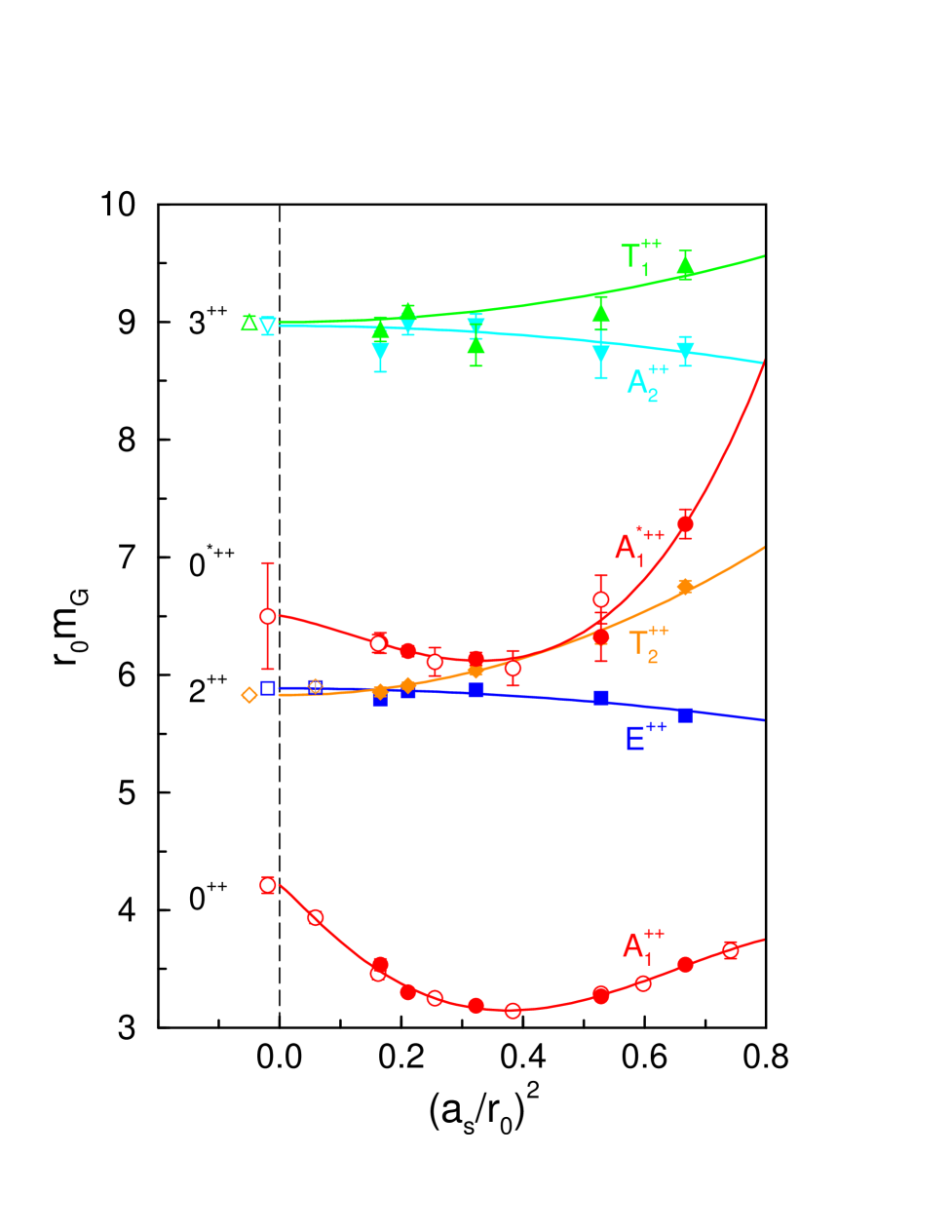
FIG. 4.: Mass estimates of the $PC=++$ glueballs in terms of $r_{0}$ against the lattice spacing $(a_{s}/r_{0})^{2}$. The solid symbols indicate results from the $\xi=5$ simulations, and the open symbols on the right-hand side of the vertical dashed line indicate results from the $\xi=3$ simulations. The solid curves are best fits to the simulation results for each state using $\varphi_{1}(a_{s})$ from Eq. (11) for the $A_{1}^{++}$ and $A_{1}^{\ast++}$ levels and $\varphi_{0}(a_{s})$ from Eq. (9) for all other levels. The open symbols on the left-hand side of the vertical dashed line show the extrapolations to the continuum limit using the best-fit forms.

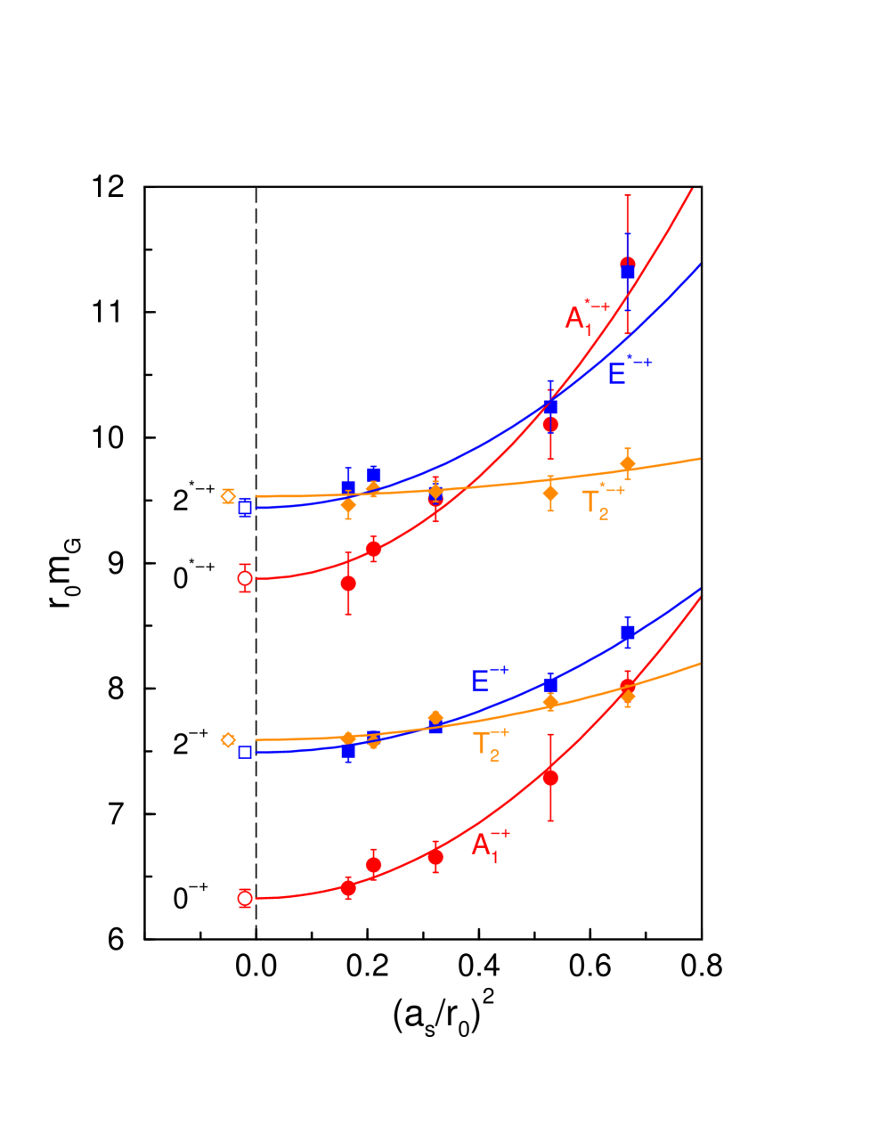
FIG. 5.: Mass estimates (solid symbols) of the $PC=-+$ glueballs in terms of $r_{0}$ against the lattice spacing $(a_{s}/r_{0})^{2}$. The solid curves are best fits of $\varphi_{0}(a_{s})$ from Eq. (9) to the results for each state; the open symbols are the continuum limit extrapolations.

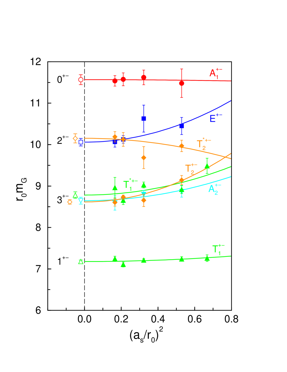
FIG. 6.: Mass estimates (solid symbols) of the $PC=+-$ glueballs in terms of $r_{0}$ against the lattice spacing $(a_{s}/r_{0})^{2}$. The solid curves are best fits of $\varphi_{0}(a_{s})$ from Eq. (9) to the results for each state; the open symbols are the continuum limit extrapolations.

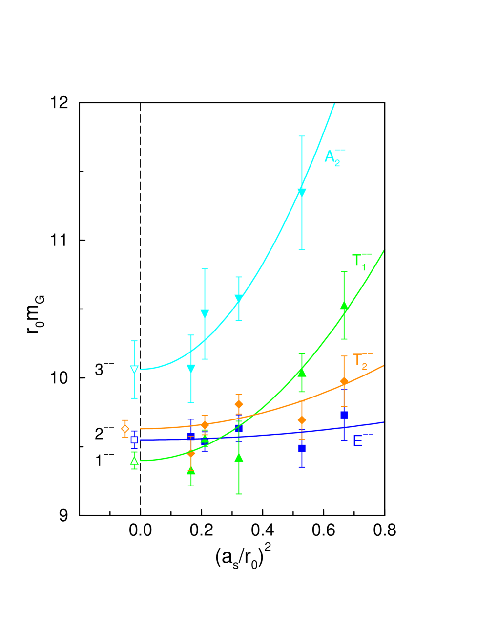
FIG. 7.: Mass estimates (solid symbols) of the $PC=--$ glueballs in terms of $r_{0}$ against the lattice spacing $(a_{s}/r_{0})^{2}$. The solid curves are best fits of $\varphi_{0}(a_{s})$ from Eq. (9) to the results for each state; the open symbols are the continuum limit extrapolations.

From perturbation theory, the leading discretization errors in our action are expected to be $O(a_{t}^{2},a_{s}^{4},\alpha_{s}a_{s}^{2})$. The agreement of the $A_{1}^{++}$, $A_{1}^{\ast++}$, $E^{++}$, $T_{2}^{++}$, and $T_{1}^{+-}$ glueball masses extracted using $\xi=3$ and $\xi=5$ (see Figs. 12 and 14 in Ref. [1]) suggests that the $O(a_{t}^{2})$ errors are negligible. Some evidence for the smallness of the $O(\alpha_{s}a_{s}^{2})$ errors comes from our earlier glueball simulations[9] which used the one-loop improved Lüscher-Weisz action[10]. After tadpole improvement, the radiative corrections to the couplings in this action were found to be very small. For these reasons, we expect that the $O(a_{t}^{2},\alpha_{s}a_{s}^{2})$ errors will be negligible compared to the $O(a_{s}^{4})$ errors.

In assuming $a_{s}/a_{t}=\xi$ (where $\xi$ is the input anisotropy parameter in the action), we introduce $O(\alpha_{s})$ errors in our estimates of the glueball masses multiplied by $r_{0}$. (Note that these errors do not enter into ratios of the glueball masses.) Such errors can be avoided by instead setting $a_{s}/a_{t}$ in a more physically motivated fashion, such as by comparing the spatial and temporal length scales extracted from appropriate correlation functions. We can also use perturbation theory to adjust the couplings in our action to remove these errors order by order in $\alpha_{s}$. However, we estimated the errors caused by imposing $a_{s}/a_{t}=\xi$ (see below) and found them to be too small to warrant the additional complexity of another $a_{s}/a_{t}$-setting scheme or the effort required to calculate the one-loop corrections to the action. A simpler approach is to incorporate the $O(\alpha_{s})$ anisotropy errors into our continuum limit extrapolations. Unfortunately, their dependence on $a_{s}$ is not well known and, as we shall see, they are generally smaller than the much more rapidly varying $O(a_{s}^{4})$ errors. Detecting their effects in a fit to about five data points for $a_{s}$ from 0.2 to 0.4 fm is not feasible. Thus, we decided to adopt the following approach: to extrapolate assuming $O(a_{s}^{4})$ errors only, then include a systematic uncertainty in our continuum-limit results from the $O(\alpha_{s})$ anisotropy errors.

One way to estimate this uncertainty is to compare measurements of the static-quark potential extracted from Wilson loops taken along the different spatial and temporal axes of the lattice[11]. The anisotropy errors can be quantified by defining $a_{s}/a_{t}$ in terms of these different potentials and comparing the result to $\xi$. If we denote the determination of the aspect ratio from the potentials by $[a_{s}/a_{t}]_{V}$ and define $Z_{\xi}$ by the relation $[a_{s}/a_{t}]_{V}=Z_{\xi}\xi$, then the deviation of $Z_{\xi}$ from unity gives us a measure of the fractional error from assuming $a_{s}/a_{t}=\xi$. The effect of these errors is to modify the multiplicative $r_{0}/a_{t}$ factors used to convert the simulation results given in terms of $a_{t}^{-1}$ into units of $r_{0}^{-1}$ suitable for extrapolation. Using the functional dependence of $r_{0}/a_{t}$ on $\xi$ from a fit to the static-quark potential, we determine that $(Z_{\xi}-1)/2$ gives us an estimate of the fractional uncertainty in our continuum limit results from the aspect ratio errors. Without mean-link improvement, $Z_{\xi}$ can deviate from unity by as much as $30\%$. When the action includes mean-link factors, the corrections are found to be small, typically a few per cent. For example, for the $\beta=2.4$, $\xi=5$ run, we obtained $Z_{\xi}=0.987(8)$; for $\beta=3.0$, $\xi=3$, an estimate of $Z_{\xi}=0.99(1)$ was found. If we assign a conservative $2\%$ error from $Z_{\xi}$, then this amounts to a $1\%$ systematic uncertainty in our continuum-limit results from the anisotropy errors.

Another way to estimate the errors due to the aspect ratio is from the perturbative calculation of $Z_{\xi}$ using the anisotropic Wilson action (the analogous calculation using $S_{I\!I}$ has not yet been done). Modifying the results from Ref. [12] to include tadpole improvement factors and writing the mean-link parameter $u_{s}=1-\alpha_{s}u_{s}^{(2)}(\xi)+O(\alpha_{s}^{2})$, one finds

$$Z_{\xi}=1+\alpha_{s}\,\left\{2\pi\left[c_{\tau}(\xi)\!-\!c_{\sigma}(\xi)\right]+u_{s}^{(2)}(\xi)\right\}+O(\alpha_{s}^{2}),$$ (8)

where the values for $c_{\tau}(\xi)$ and $c_{\sigma}(\xi)$ can be obtained from Fig. 1 in Ref. [12]. From this equation, one sees that when $\xi=3-5$ and $\alpha_{s}\sim 0.2$, the aspect ratio receives less than a $2\%$ correction; if the tadpole improvement factor $u_{s}^{(2)}(\xi)$ is omitted, a large $30\%$ correction is found. For the improved action $S_{I\!I}$, we expect that these values should be somewhat smaller. Again, we can assign a conservative $2\%$ error in $Z_{\xi}$ to obtain a $1\%$ systematic uncertainty in our continuum estimates.

To summarize, our approach is to extrapolate to the continuum limit using

$$\varphi_{0}(a_{s})=r_{0}m_{G}+c_{4}\ \frac{a_{s}^{4}}{r_{0}^{4}},$$ (9)

where $r_{0}m_{G}$ and $c_{4}$ are the best-fit parameters, then add a $1\%$ systematic uncertainty from the $O(\alpha_{s})$ anisotropy errors. Eq. (9) worked well in all cases except for the $A_{1}^{++}$ and $A_{1}^{\ast++}$ levels. The best-fit curves using Eq. (9) are shown in Figs. 4-7; the extrapolations of these curves to the continuum limit are indicated in these figures by the open symbols on the left-hand sides of the vertical dashed lines. Note that the extrapolation uncertainties shown in these plots do not yet include the systematic anisotropy error.

As discussed in Ref. [1], our results for the $A_{1}^{++}$ and $A_{1}^{\ast++}$ levels remain problematical. These levels have large finite-lattice-spacing errors which do not obey Eq. (9). There is growing evidence that these large discretization errors are due to the presence of a critical end point of a line of phase transitions (not corresponding to any physical transition found in QCD) in the fundamental-adjoint coupling plane[13, 14, 15]. It has been conjectured that this critical point defines the continuum limit of a $\phi^{4}$ scalar field theory[14]. As one nears this critical point, the coherence length in the scalar channel becomes large, which means that the mass gap in this channel becomes small; all other observables, including glueball masses, appear to be affected to a much lesser extent. The effect of this critical point on the functional form of the discretization errors in the scalar glueball mass is not well known, so we must proceed somewhat empirically. One possibility is that the critical point might enhance the perturbative $O(\alpha_{s})$ errors; another is that it may induce an $O(a_{s}^{2})$ error which would not otherwise be present. We fit several simple functions to the $A_{1}^{++}$ mass results and found that the following two functions worked very well:

$$\varphi_{1}(a_{s}) = r_{0}m_{G}+c_{4}\ \frac{a_{s}^{4}}{r_{0}^{4}}$$ (11)

$$-\left(d_{2}\ \frac{a_{s}^{2}}{r_{0}^{2}}+d_{4}\ \frac{a_{s}^{4}}{r_{0}^{4}}\right)\bigl{[}\ln(a_{s}\Lambda)\bigr{]}^{-1},$$

$$\varphi_{2}(a_{s}) = r_{0}m_{G}+c_{2}\ \frac{a_{s}^{2}}{r_{0}^{2}}+c_{4}\ \frac{a_{s}^{4}}{r_{0}^{4}}+c_{6}\ \frac{a_{s}^{6}}{r_{0}^{6}},$$ (12)

where $r_{0}m_{G}$, $c_{4}$, $c_{6}$, $d_{2}$, and $d_{4}$ are the best-fit parameters. Eq. (12) is simply a cubic polynomial in $(a_{s}/r_{0})^{2}$. Eq. (11) incorporates the expected leading dependence on the QCD coupling $\alpha_{s}(a_{s})\sim-1/\ln(a_{s}\Lambda)$ up to $O(a_{s}^{4})$. Various estimates of the QCD scale parameter $\Lambda_{\overline{\rm MS}}$ suggest that $r_{0}\Lambda_{\overline{\rm MS}}\sim 0.6$. Hence, we used $r_{0}\Lambda=0.5$ and verified that our continuum limit estimates were insensitive to the choice of $r_{0}\Lambda$ in the range from about 0.3 to 0.8. Both the $d_{2}$ and $d_{4}$ terms were needed to achieve this insensitivity.

The best-fit curves using Eq. (11) are shown in Fig. 4. The best fit to the $A_{1}^{++}$ results has $\chi^{2}/N_{\rm DF}=0.57$, and for the $A_{1}^{\ast++}$, we find $\chi^{2}/N_{\rm DF}=0.35$. The extrapolation of these curves to the continuum limit yields $r_{0}m({A_{1}^{++}})=4.21(7)$ and $r_{0}m({A_{1}^{\ast++}})=6.50(44)$. Using Eq. (12), we obtain $r_{0}m({A_{1}^{++}})=4.30(8)$ with $\chi^{2}/N_{\rm DF}=0.53$ and $r_{0}m({A_{1}^{\ast++}})=6.52(54)$ with $\chi^{2}/N_{\rm DF}=0.35$ Since $\varphi_{1}(a_{s})$ was more closely connected to a perturbative analysis, we chose the estimates obtained using Eq. (11) for our final results, but added the differences between the two extrapolations as a systematic error. After including an additional $1\%$ anisotropy error, we end up with $r_{0}m(A_{1}^{++})=4.21(12)$ and $r_{0}m(A_{1}^{\ast++})=6.50(45)$.

Note that the $A_{1}^{++}$ estimate differs slightly from our earlier estimate of $3.98(15)$ given in Ref. [1]. Our previous extrapolation suffered from the absence of a mass measurement at a lattice spacing smaller than 0.2 fm; the need for such a measurement to obtain a reliable continuum limit estimate for this level was acknowledged in Ref. [1]. The current study includes a new measurement at a lattice spacing near 0.1 fm; the inclusion of this new measurement is responsible for the slight difference in the two extrapolations. Note that our improved estimate $4.21(12)$ agrees very well with the value $4.33(5)$ obtained by extrapolating existing Wilson action data for the scalar glueball mass. Unfortunately, the mass of the $A_{1}^{\ast++}$ is very poorly determined because a measurement of the $A_{1}^{\ast++}$ mass was not obtained in the $\beta=3.0$, $\xi=3$ simulation.

Recently, we have demonstrated that the discretization errors in the scalar glueball mass can be dramatically reduced by simulating with an action which includes an additional two-plaquette interaction[15]. With such an action, we should be able to substantially improve upon our determinations of the scalar-channel glueball masses in the near future. A study in SU(2) lattice gauge theory[16] has also shown that lattice-spacing errors in the scalar glueball can be reduced by using the mean spatial and temporal links in Landau gauge for the values of the link variable renormalization parameters $u_{s}$ and $u_{t}$, respectively.

B Spin identification

The last step in our calculation of the glueball spectrum is to identify the continuum spin content of each level. This is done by matching the observed patterns of degeneracies in the levels from different $O_{h}^{C}$ representations to those expected for the various continuum $J^{PC}$ states. For example, a $J=0$ state occurs only in the $A_{1}$ representation of $O$, a $J=2$ state occurs in both the $E$ and $T_{2}$ representations, and a state of $J=3$ gets split across the $A_{2}$, $T_{1}$, and $T_{2}$ representations. The numbers of times that the irreducible representations of the octahedral group $O$ occur in the subduced representations $J\downarrow O$ of the rotation group $SO(3)$ restricted to the subgroup $O$ are listed in Table VI. Given the values in this table and either the continuum limit estimates in Figs. 4-7 or the results shown in Fig. 2, we can then deduce the continuum spin quantum numbers.

TABLE VI.: Number of times each irreducible representation of the octahedral group $O$ occurs in the subduced representations $J\downarrow O$ of the rotation group $SO(3)$ restricted to subgroup $O$.

$J$	$A_{1}$	$A_{2}$	$E$	$T_{1}$	$T_{2}$
0	1	0	0	0	0
1	0	0	0	1	0
2	0	0	1	0	1
3	0	1	0	1	1
4	1	0	1	1	1
5	0	0	1	2	1
6	1	1	1	1	2
7	0	1	1	2	2
8	1	0	2	2	2
9	1	1	1	3	2
10	1	1	2	2	3
11	0	1	2	3	3
12	2	1	2	3	3

Consider first the $PC=++$ sector. The $A_{1}^{++}$ state is not degenerate with any other level; hence, it can be identified as a $J=0$ state. The $E^{++}$ and $T_{2}^{++}$ states are degenerate, implying that they correspond to the five polarizations of a $J=2$ glueball. The $A_{1}^{\ast++}$ state is seen to have no degenerate partners, suggesting a $J=0$ excited state. The $A_{2}^{++}$ state can correspond to $J=3,6,7,9,\dots$. For all of these $J$ values, there should be an accompanying level in the $T_{1}^{++}$ channel, and such a level is observed. We conclude that the $A_{2}^{++}$ and $T_{1}^{++}$ states correspond most likely to a $J=3$ state, but less likely $J=6,7,9,\dots$ interpretations cannot be ruled out. The $J=3$ assignment is also supported by model predictions, discussed in Sec. VI.

In the $PC=-+$ sector, the $A_{1}^{-+}$ and $A_{1}^{\ast-+}$ states are easily identified with $J=0$ states, and the degenerate $E^{-+}$ and $T_{2}^{-+}$ states must correspond to a $J=2$ glueball. The degenerate $E^{\ast-+}$ and $T_{2}^{\ast-+}$ states most likely correspond to a $J=2$ state as well, although as noted in Sec. III, the proximity of these levels to the two-glueball threshold leaves their status somewhat uncertain. Also, we cannot statistically rule out the possibility that, in combination with two states in the $T_{1}^{-+}$ irreducible representation, they are associated with a $J=5$ glueball. We cannot rule out an accompanying degenerate level in the $A_{1}^{-+}$ channel. If such a state exists, then these could be the levels corresponding to a $J=4$ or a $J=8$ glueball.

The $T_{1}^{+-}$ state must correspond to a $J=1$ glueball, and the degenerate $A_{2}^{+-}$, $T_{1}^{\ast+-}$, and $T_{2}^{+-}$ levels correspond to a $J=3$ glueball. A glueball having $J=2$ is the most likely interpretation for the degenerate $E^{+-}$ and $T_{2}^{\ast+-}$ states. However, we cannot rule out the possibility of accompanying levels in the $T_{1}^{+-}$ and $A_{2}^{+-}$ channels. Taking all possibilities into account, the alternate interpretations are $J=5,7,11$. The very high lying $A_{1}^{+-}$ can be interpreted as a $J=0$ glueball, but $J=4,6,8,\dots$ cannot be excluded.

Finally, consider the $PC=--$ sector. The most probable scenario is as follows: the $T_{1}^{--}$ corresponds to a $J=1$ glueball, the degenerate $E^{--}$ and $T_{2}^{--}$ are the five polarizations of a $J=2$ glueball, and the $A_{2}^{--}$ is a $J=3$ state. Of course, we cannot rule out the presumably higher-lying $J=6,7,9,11,\dots$ interpretations for the $A_{2}^{--}$. Another possibility is that the $E^{--}$, $T_{1}^{--}$, and $T_{2}^{--}$ are degenerate, in which case they could correspond to a $J=5$ glueball. Even less likely is that all four levels are degenerate. In this case, one could interpret them as a single $J=7$ or $J=11$ state, or as accidentally degenerate $J=3$ and $J=2$ glueballs. However, all higher-spin interpretations would require a degenerate ground state in either the $T_{1}^{--}$ or $T_{2}^{--}$ channel. Our correlator fits suggest these degeneracies are missing, making $J=5,6,7\dots$ interpretations unlikely.

VI Results and discussion

TABLE VII.: Final continuum-limit glueball mass estimates $m_{G}$. When a unique $J$ interpretation for a state cannot be made, the other possibilities are indicated in the second column. States whose interpretation requires further study are indicated by a dagger. In column 3, the first error is the statistical uncertainty from the continuum-limit extrapolation and the second is the estimated uncertainty from the anisotropy. In the final column, the first error comes from the combined uncertainties in $r_{0}m_{G}$, the second from the uncertainty in $r_{0}^{-1}=410(20)$ MeV.

$J^{PC}$	Other $J$	$r_{0}m_{G}$	$m_{G}$ (MeV)
$0^{++}$		4.21 (11)(4)	1730 (50)  (80)
$2^{++}$		5.85 (2)  (6)	2400 (25)  (120)
$0^{-+}$		6.33 (7)  (6)	2590 (40)  (130)
$0^{*++}$		6.50 (44)(7)†	2670 (180)(130)
$1^{+-}$		7.18 (4)  (7)	2940 (30)  (140)
$2^{-+}$		7.55 (3)  (8)	3100 (30)  (150)
$3^{+-}$		8.66 (4)  (9)	3550 (40)  (170)
$0^{*-+}$		8.88 (11)(9)	3640 (60)  (180)
$3^{++}$	$6,7,9,\dots$	8.99 (4)  (9)	3690 (40)  (180)
$1^{--}$	$3,5,7,\dots$	9.40 (6)  (9)	3850 (50)  (190)
$2^{*-+}$	$4,5,8,\dots$	9.50 (4)  (9)†	3890 (40)  (190)
$2^{--}$	$3,5,7,\dots$	9.59 (4)  (10)	3930 (40)  (190)
$3^{--}$	$6,7,9,\dots$	10.06 (21)(10)	4130 (90)  (200)
$2^{+-}$	$5,7,11,\dots$	10.10 (7)  (10)	4140 (50)  (200)
$0^{+-}$	$4,6,8,\dots$	11.57 (12)(12)	4740 (70)  (230)

Our final results for the glueball spectrum in terms of $r_{0}$ are given in Table VII. In this table, we assumed the most likely spin interpretations as described in the previous section and accordingly combined the continuum limit extrapolations (shown as open symbols on the left-hand sides of the vertical dashed lines in Figs. 4-7), then added the $1\%$ anisotropy error, to obtain final estimates for the glueball masses in terms of $r_{0}$. The combinations used to obtain these estimates are also indicated in Figs. 4-7 by the $J^{PC}$ labels near the left vertical axes. Wherever applicable, we have also indicated in Table VII any alternative spin interpretations which cannot be ruled out. These final estimates are also shown in Fig. 8. The $0^{\ast++}$ and $2^{\ast-+}$ states are shown as dashed hollow boxes to indicate that their interpretations as glueballs are tentative. Our concern about the $0^{\ast++}$ state stems from its non-negligible finite volume effects; for the $2^{\ast-+}$ state, its nearness to the two-glueball threshold in our simulations is worrisome. Note that our estimates $r_{0}m(0^{++})=4.21(12)$ and $r_{0}m(2^{++})=5.85(6)$ agree very well with $4.33(5)$ and $6.0(1)$, respectively, obtained by extrapolating the Wilson action simulation results from Refs. [2, 3, 17, 18] to the continuum limit. Several glueball mass ratios are presented in Table VIII. We can determine these ratios very accurately since, as noted earlier, they are not contaminated by anisotropy errors. The uncertainties given in Table VIII are calculated using the empirical fact that correlations between different symmetry channels were found to be negligible. Note that the pseudoscalar glueball is clearly resolved (at the $7\sigma$ level) to be heavier than the tensor.

TABLE VIII.: Glueball mass ratios.

$m(2^{++})/m(0^{++})$	$1.39(4)$
$m(0^{-+})/m(0^{++})$	$1.50(4)$
$m(0^{\ast++})/m(0^{++})$	$1.54(11)$
$m(1^{+-})/m(0^{++})$	$1.70(5)$
$m(2^{-+})/m(0^{++})$	$1.79(5)$
$m(3^{+-})/m(0^{++})$	$2.06(6)$
$m(0^{\ast-+})$/$m(0^{++})$	$2.11(6)$
$m(0^{-+})$ /$m(2^{++})$	$1.081(12)$

All of the glueball states shown in Fig. 8 are stable against decay to lighter glueballs. In the $PC=++$ sector, the threshold for decay into two identical $0^{++}$ glueballs having zero total momentum is at twice the mass of the scalar glueball. Although this lies below the mass of the $3^{++}$ glueball, Bose symmetrization prohibits odd $L$ partial waves, where $L$ is the relative orbital angular momentum, so that the $3^{++}$ glueball cannot decay into two identical scalar glueballs. In the $PC=-+$ sector, the lowest-lying two-glueball state consists of the $0^{++}$ and $2^{++}$ glueballs in a relative $P$-wave; all of our glueballs in this sector have masses below the sum of the scalar and tensor glueball masses. States of total zero momentum and comprised of the $0^{++}$ and $1^{+-}$ glueballs with relative orbital angular momentum $L$ are the lowest-lying two-glueball states in the $PC=+-$ sector when $L$ is even and in the $PC=--$ sector when $L$ is odd. Only the $0^{+-}$ glueball has sufficient mass to decay into two such glueballs; however, this decay is forbidden because $L=1$ is required to make a state of zero total angular momentum.

To convert our glueball masses into physical units, the value of the hadronic scale $r_{0}$ must be specified. We used $r_{0}^{-1}=410(20)$ MeV from Ref. [1] to obtain the scale shown on the right-hand vertical axis of Fig. 8. This estimate was obtained by combining Wilson action calculations of $a/r_{0}$ with values of the lattice spacing $a$ determined using quenched simulation results of various physical quantities, such as the masses of the $\rho$ and $\phi$ mesons, the decay constant $f_{\pi}$, and the $1P-1S$ splittings in charmonium and bottomonium. Note that the errors shown in Fig. 8 do not include the uncertainty in $r_{0}^{-1}$. For the lowest-lying glueballs, we obtain $m(0^{++})=1730(50)(80)$ MeV and $m(2^{++})=2400(25)(120)$ MeV, where the first error comes from the uncertainty in $r_{0}m_{G}$ and the second error comes from the uncertainty in $r_{0}^{-1}$. A great deal of care should be taken in making direct comparisons with experiment since these values neglect the effects of light quarks and mixings with nearby conventional mesons. It is this mixing which has made the search for an incontrovertible experimental signal so difficult. A glueball having exotic $J^{PC}$ will not mix with conventional hadrons and would be ideal for establishing the existence of glueballs. Unfortunately, our results indicate that the lightest such state, the $2^{+-}$ glueball, has a mass greater than 4 GeV.

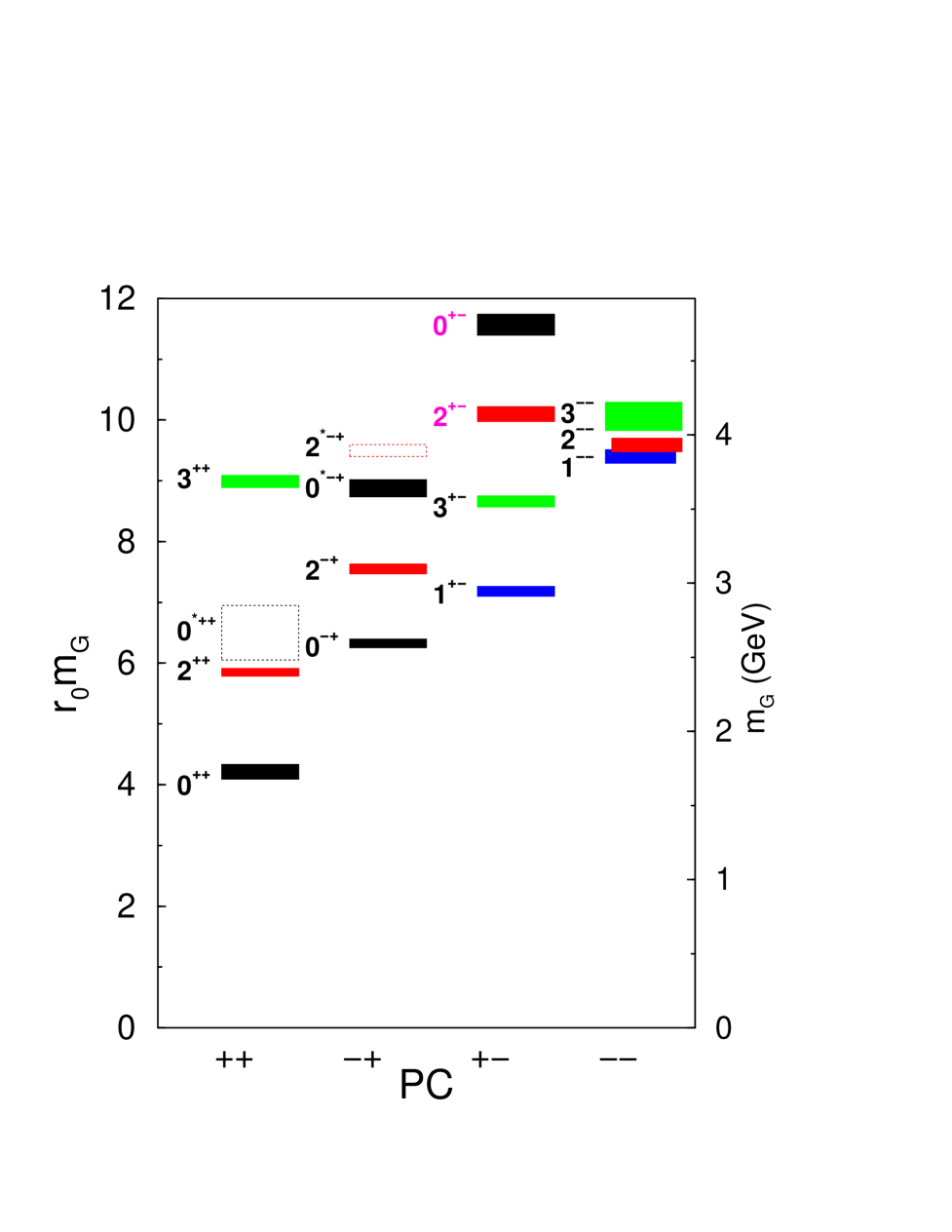
FIG. 8.: The mass spectrum of glueballs in the pure SU(3) gauge theory. The masses are given in terms of the hadronic scale $r_{0}$ along the left vertical axis and in terms of GeV along the right vertical axis (assuming $r_{0}^{-1}=410$ MeV). The mass uncertainties indicated by the vertical extents of the boxes do not include the uncertainty in setting $r_{0}$. The locations of states whose interpretation requires further study are indicated by the dashed hollow boxes.

Kuti has recently pointed out[19] that the glueball spectrum shown in Fig. 8 can be qualitatively understood in terms of the interpolating operators of minimal dimension which can create glueball states. With the expectation that higher dimensional operators create higher mass states, the authors in Ref. [20], following an approach suggested in Refs. [21, 22], constructed all operators of dimension $4$, $5$, and $6$ capable of creating glueballs from the QCD vacuum. Such operators are gauge-invariant combinations of the chromoelectric and chromomagnetic fields; operators equivalent to a total derivative or related to a conserved current are excluded. The lowest dimensional operators capable of creating glueballs are of dimension four and have the form ${\rm Tr}F_{\mu\nu}F_{\alpha\beta}$, where $F_{\mu\nu}$ is the gauge field strength tensor; these operators create glueballs with $J^{PC}=0^{++},2^{++},0^{-+}$ and $2^{-+}$. The dimension five operators of the form ${\rm Tr}F_{\mu\nu}D_{\delta}F_{\alpha\beta}$, where $D_{\mu}$ is the covariant derivative, produce only two new glueball states having $J^{PC}=1^{++}$ and $3^{++}$. At dimension six, operators of the form ${\rm Tr}F_{\mu\nu}F_{\alpha\beta}F_{\delta\sigma}$ produce $J^{PC}=0^{\pm+},1^{\pm\pm},2^{\pm\pm}$, and $3^{\pm-}$; operators of the form ${\rm Tr}F_{\mu\nu}\{D_{\alpha},D_{\beta}\}F_{\delta\sigma}$ produce $J^{PC}=1^{-+},3^{-+}$, and $4^{\pm+}$. Of course, this ordering should not be taken too quantitatively, but we find that the method provides a reasonably satisfactory explanation of the observed spectrum, especially given the simplicity of the approach. Of the lightest six states we resolve, four have the quantum numbers expected from the dimension-four interpolating operators. The method also explains the absence of any low-lying $0^{\pm-}$ and $1^{-+}$ glueballs.

The spectrum of Fig. 8 can also be reasonably well explained in terms of a simple constituent gluon model in which the fundamental gluon field is replaced by the Hartree modes of a constituent field with residual perturbative interactions; the Hartree modes are taken to be the modes of a free gluon inside a spherical cavity with confining boundary conditions. Such a (bag) model has been recently revisited in Ref. [19]. Using values for $\alpha_{s}$ and the bag pressure appropriate for heavy-quark spectroscopy and the static-quark potential, remarkable agreement with the observed levels of Fig. 8 was found.

VII Conclusion

In this paper, we used numerical simulations of gluons on spatially-coarse, temporally-fine lattices to significantly improve our knowledge of the glueball spectrum in SU(3) Yang-Mills theory. This is an important step towards understanding glueballs in the real world. Six simulations for spatial grid separations ranging from 0.1 to 0.4 fm were performed on DEC Alpha and Sun Ultrasparc workstations. Care was taken to differentiate single glueball states from unwanted two-glueball and torelon-pair states. An additional small-volume simulation assisted in the identification of the single glueball states and demonstrated the smallness of systematic errors from finite volume. The simulation results were extrapolated to the continuum limit and the continuum spin quantum numbers were identified. The end result, shown in Fig. 8, was a nearly complete survey of the glueball spectrum in the pure glue theory below 4 GeV. A total of thirteen glueballs were found, and two other tentative candidates were also located.

In the future, we plan to improve our determinations of the scalar-channel glueballs by simulating with an action that includes an additional two-plaquette interaction. We also intend to extend our anisotropic lattice technology to include quarks. With the help of femto-universe techniques, we hope ultimately to investigate the properties of glueballs in reality.

REFERENCES

- [1] C. Morningstar and M. Peardon, Phys. Rev. D56, 4043 (1997).
- [2] G. Bali et al. (UKQCD Collaboration), Phys. Lett. B 309, 378 (1993).
- [3] C. Michael and M. Teper, Nucl. Phys. B314, 347 (1989).
- [4] B. Berg and A. Billoire, Nucl. Phys. B221, 109 (1983); B226, 405 (1983).
- [5] G.P. Lepage and P.B. Mackenzie, Phys. Rev. D 48, 2250 (1993).
- [6] A.M. Schönfliess, Krystallsysteme und Krystallstructur (Druck und Verlag von B.G. Teubner, Leipzig, 1891).
- [7] See, for example, J. F. Cornwell, Group Theory in Physics (Academic Press, London, 1984), Vol. I.
- [8] R. Sommer, Nucl. Phys. B411, 839 (1994).
- [9] C. Morningstar and M. Peardon, in Lattice ’95, Proceedings of the International Symposium, Melbourne, Australia, edited by T.D. Kieu et al. [Nucl. Phys. B (Proc. Suppl.) B47, 258 (1996)].
- [10] M. Lüscher and P. Weisz, Phys. Lett. 158B, 250 (1985).
- [11] C. Morningstar, in Lattice ’96, Proceedings of the International Symposium, St. Louis, Missouri, edited by C. Bernard et al. [Nucl. Phys. B (Proc. Suppl.) B53, 914 (1997)].
- [12] F. Karsch, Nucl. Phys. B205, 285 (1982).
- [13] A. Patel et al., Phys. Rev. Lett. 57, 1288 (1986).
- [14] U. Heller, Phys. Lett. B 362, 123 (1995).
- [15] C. Morningstar and M. Peardon, in Lattice ’98, Proceedings of the International Symposium, Boulder, Colorado, edited by T. DeGrand et al., to appear (hep-lat/9808045).
- [16] N. Shakespeare and H. Trottier, Phys. Rev. D 59, 014502 (1999).
- [17] H. Chen et al., in Lattice ’93, Proceedings of the International Symposium, Dallas, Texas, edited by T. Draper et al. [Nucl. Phys. B (Proc. Suppl.) 34, 357 (1994)].
- [18] P. de Forcrand et al., Phys. Lett. 160B, 137 (1985).
- [19] J. Kuti, in Lattice ’98 [15], to appear (hep-lat/9811021).
- [20] R.L. Jaffe, K. Johnson, and Z. Ryzak, Ann. Phys. 168, 344 (1986).
- [21] H. Fritzsch and P. Minkowski, Nuovo Cim. 30A, 393 (1975).
- [22] J.D. Bjorken, in Proceedings of the 1979 SLAC Summer Institute on Particle Physics, Stanford, California, p. 219.