1 Introduction

Discretized models of $D$–dimensional Euclidean quantum gravity, known as simplicial gravity or dynamical triangulations, have been extensively studied in the past decade. The two dimensional model was proposed quite some time ago in Ref. [2], and generalized to three and four dimensions in Ref. [3, 4]. The model is defined by the grand-canonical partition function

$${\cal Z}(\mu,\kappa_{0})=\sum_{N_{D}}e^{\textstyle\;-\mu N_{D}}Z(\kappa_{0},N_{D})$$ (1)

where $\mu$ and $\kappa_{0}$ are the discrete cosmological and inverse Newton’s constants, $N_{D}$ is the number of $D$–dimensional simplices, and $Z(\kappa_{0},N_{D})$ is the canonical partition function

$$Z(\kappa_{0},N_{D})\;=\;\sum_{N_{0}}\,{\rm e}^{\textstyle\;\kappa_{0}N_{0}}\;W_{D}(N_{0},N_{D})\;.$$ (2)

The micro-canonical partition function, $W_{D}$, is defined as

$$W_{D}(N_{0},N_{D})\;=\!\!\sum_{T\in{\cal T}(N_{0},N_{D})}\;\frac{1}{C_{T}}\,\,=\,\frac{1}{N_{0}!}\,\sum_{L\in{\cal L}(N_{0},N_{D})}1\;,$$ (3)

where the sum is over an ensemble of combinatorial triangulations ${\cal T}$ with a spherical topology and with $N_{0}$ vertices and $N_{D}$ $D$–simplices. For $D>2$ these two numbers are independent. The symmetry factor $C_{T}$ of a triangulation $T$ is given by the number of equivalent labeling of the vertices. Including this factor is equivalent to summing over all labeled triangulations ${\cal L}(N_{0},N_{D})$.

As a statistical system simplicial gravity displays a wealth of intriguing features. In $D>2$ it exhibits a geometric phase transition separating a strong-coupling crumpled phase, where the internal geometry of the triangulations collapses, from a weak-coupling elongated phase characterized by triangulations consisting of “bubbles” glued together into a tree-like structure or branched polymers [5]. Both in three [4] and four dimensions [6] this transition is discontinuous.

In the absence of a continuous phase transition with a divergent correlation length any sensible continuum limit where a theory of gravity might be defined appears to be ruled out. This has led to the studies of modified models of simplicial gravity, e.g. by changing the relative weight of the triangulations with a modified measure [7], or by coupling matter fields to the theory [8]. Suitable modified the phase structure of the model changes; the polymerization of the geometry in the weak-coupling limit — the elongated phase — is suppressed and a new crinkled phase appears [9]. The crinkled phase is separated from the other two phases by lines of either a soft continuous phase transitions, or possible a cross-over (a divergent specific heat is not observed). Qualitatively the same phase structure, shown schematically in Figure 1, is observed both in three and four dimensions.

Both in the elongated and in the crinkled phase the canonical partition function is seen to have the asymptotic behavior

$$Z(\kappa_{0},N_{D})\;\sim\;{\rm e}^{\textstyle\;\mu_{c}N_{D}}\;N_{D}^{\textstyle\gamma-3}\;,$$ (4)

which defines the string susceptibility exponent $\gamma$. In the crumpled phase, on the other hand, the sub-leading behavior is exponential, corresponding to $\gamma=-\infty$.

Figure 1: A schematic phase diagram of modified simplicial quantum gravity for $D>2$. The solid line indicates discontinuous phase transitions, the dashed lines are either soft continuous transitions or a cross-over.

Many of the properties of the model Eq. (1), in the weak-coupling regime $\kappa_{0}~{}\!>~{}\!\kappa_{0}^{c}$, are reflected by triangulations close to the upper kinematic bound $N_{0}/N_{D}=n_{0}^{max}$. This is evident both from Monte Carlo (MC) simulations and from the analysis of a strong-coupling expansion (SCE) of the partition function. For combinatorial triangulations, where each simplex is uniquely defined by a set of $\bigl{(}D+1\bigr{)}$ distinct vertices, the upper kinematic bound is $n_{0}^{\it max}=1/D$. Although this bound is only saturated in the thermodynamic limit, $N_{D}\rightarrow\infty$, for each finite volume there exist triangulations with a well-defined maximal number of vertexes $N_{0}^{\it max}(N_{D})$. The ensemble of these triangulations, the maximal ensemble ${\cal T}_{\it max}$, defines the micro-canonical partition function

$$W_{max}(N_{D})\;\equiv\;W_{D}\bigl{(}N_{0}^{max}(N_{D}),N_{D}\bigr{)}\;=\;\sum_{T\in{\cal T}_{max}(N_{D})}\;\frac{1}{C_{T}}\;.$$ (5)

In this paper we investigate the properties of the maximal ensemble, mostly restricted to three dimensions, using both MC simulations and a SCE, i.e. a direct enumeration of the micro-canonical partition function Eq. (5). This investigation is separated into two parts. In the first part we study the pure (un-modified) ensemble and show that $W_{max}(N_{3})$ effectively separates into three distinct series (or two series in $4D$) as in general there are several different volumes $N_{D}$ corresponding to a given $N_{0}^{max}$. One of those series is an ensemble of stacked spheres, a particular simple class of triangulations which can be enumerated exactly. This we do in Section 3.

The other two series can be considered as “almost” stacked spheres, i.e. with one, or two, defects respectively. Heuristic arguments, supported by numerical evidence, show that although the leading asymptotic behavior of the three series is identical, the effect of inserting a defect increases the exponent $\gamma$ by $+1$ (or $+2$) compared to stacked spheres. This is discussed in Section 4.

In the second part of the paper, Section 5, we study the model Eq. (5) with a modified measure,

$$W_{max}(N_{D},\beta)\;=\;\sum_{T\in{\cal T}_{max}}\;\frac{1}{C_{T}}\;\prod_{i=1}^{N_{0}}\;q_{i}^{\;\beta}\;.$$ (6)

Here $q_{i}$ is the order of a vertex $i$, i.e. the number of simplices incident to that vertex. As the measure is modified, varying $\beta$, we observe a soft geometric phase transition from the elongated phase to a crinkled phase for $\beta\lesssim-1$, in agreement with the phase diagram Figure 1. Moreover, a scaling analysis of the transition is consistent with a third order transition ($\alpha=-1$).

In the crinkled phase the fractal structure is dominated by a gas of sub-singular vertices, i.e. vertices whose order grows sub-linearly with the volume. The intrinsic fractal structure is characterized by a set of critical exponents: (i) A negative string susceptibility exponent $\gamma$, which decreases with $\beta$. (ii) A Hausdorff dimension which is either $d_{H}=\infty$, or $d_{H}^{\prime}\approx 2$ (as $\beta\rightarrow-\infty$), depending on whether it is measured on the triangulation itself or its dual graph. (iii) A spectral dimension, measured on the dual graph, which increases smoothly from a branched polymer value $d_{s}=4/3$, at $\beta=0$, to $d_{s}\approx 3/2$ at $\beta=-4$.

We have collected some of the more technical issues in two appendixes: In Appendix A we list the SCE of the three different series, and in Appendix B we describe some complications in extracting $\gamma$ from measurements of minbu distributions on maximal triangulations.

2 Maximal triangulations

A maximal triangulation is a triangulation which for given volume $N_{D}$ has the maximal allowed number of vertices $N_{0}$. For a combinatorial triangulation this implies:

$$N_{0}^{max}\;=\;\left\{\begin{array}[]{cc}\left\lfloor\frac{\textstyle N_{3}+10}{\textstyle 3}\right\rfloor&D=3\;,\\ \\ \left\lfloor\frac{\textstyle N_{4}+18}{\textstyle 4}\right\rfloor&D=4\;.\end{array}\right.$$ (7)

Here $\lfloor x\rfloor$ denotes the floor function, i.e. the biggest integer not greater than $x$. From this definition it follows that in general more then one volume will correspond to a given maximal vertex number. In $3D$ this defines three different series, labeled by the $\bigl{(}N_{0},N_{3}\bigr{)}$–pairs:

$$S^{0}\;\bigl{(}N_{0},3N_{0}\!-\!10\bigr{)},\qquad S^{1}\;\bigl{(}N_{0},3N_{0}\!-\!9\bigr{)},\qquad{\rm and}\qquad S^{2}\;\bigl{(}N_{0},3N_{0}\!-\!8\bigr{)}.$$ (8)

The first series $S^{0}$ has the smallest volume for a given number of vertices and we will call it the minimal series.

Likewise, in $4D$ there are in principle four different series. However, as only combinatorial four-triangulations of even volume are allowed this reduces to only two:

$$S^{0}\;\bigl{(}N_{0},4N_{0}\!-\!18\bigr{)}\qquad{\rm and}\qquad S^{1}\;\bigl{(}N_{0},4N_{0}\!-\!17\bigr{)}.$$ (9)

In the space of all triangulations, the different series are related through a set of (topology preserving) geometric changes, the $\bigl{(}p,q\bigr{)}$–moves. In a $\bigl{(}p,q\bigr{)}$–move, where $p=D+1-q$, a ($q-1$)–sub-simplex is replaced by its “dual“ ($p-1$)–sub-simplex, provided no manifold constraint is violated. These moves are used in the MC simulations and are ergodic for $D\leq 4$, i.e. any two triangulations are related through a finite sequence of moves [10].

Figure 2: The ($p,q$)–moves in three dimensions: (a) Inserting a vertex and its inverse, deleting a vertex. (b) Replacing a triangle by an link and vice verse.

In three dimensions there are two sets of moves: Move $\bigl{(}1,4\bigr{)}$ inserts a vertex into a tetrahedra and its inverse, move $\bigl{(}4,1\bigr{)}$, deletes a vertex of order four. In move $\bigl{(}2,3\bigr{)}$ a triangle separating two adjacent tetrahedra is replaced by a link connecting the opposite vertices. This is shown in Figure 2. These moves change the number of different $D$–simplices in the following way:

$$\begin{pmatrix}N_{0}\\ N_{1}\\ N_{2}\\ N_{3}\end{pmatrix}\,\begin{matrix}{(1,4)}\\ \rightleftarrows\\ {(4,1)}\end{matrix}\,\begin{pmatrix}N_{0}+1\\ N_{1}+4\\ N_{2}+6\\ N_{3}+3\end{pmatrix}\qquad{\rm and}\qquad\begin{pmatrix}N_{0}\\ N_{1}\\ N_{2}\\ N_{3}\end{pmatrix}\,\begin{matrix}{(2,3)}\\ \rightleftarrows\\ {(3,2)}\end{matrix}\,\begin{pmatrix}N_{0}\\ N_{1}+1\\ N_{2}+2\\ N_{3}+1\end{pmatrix}\,.$$ (10)

Note that only the first set of moves changes both the volume and the number of vertices, and when applied to a maximal triangulation we stay within the particular series, i.e. the different series are internally connected via this move.

The different series are connected, for fixed $N_{0}$, by the $\bigl{(}2,3\bigr{)}$ and the $\bigl{(}3,2\bigr{)}$–moves. However, as it is not possible to apply move $\bigl{(}3,2\bigr{)}$ to the series $S^{0}$ (as triangulations in this series have the minimal volume for a given $N_{0}$), the only connection which the maximal ensemble has with the rest of the triangulation space is via move $\bigl{(}2,3\bigr{)}$ applied to the series $S^{2}$. The relations between the different series, via the $\bigl{(}p,q\bigr{)}$–moves, are shown in Figure 3.

\psfrag{m23}{$(2,3)$}\psfrag{m32}{$(3,2)$}\psfrag{m14}{$(1,4)+(4,1)$}\psfrag{m14r}[r][r]{$(1,4)+(4,1)$}\psfrag{m14c}[c][c]{$(1,4)+(4,1)$}\psfrag{s0}{$S^{0}$}\psfrag{s1}{$S^{1}$}\psfrag{s2}{$S^{2}$}\includegraphics[width=284.52756pt]{moves.eps}

Figure 3: The relations between the different series of the $3D$ maximal ensemble, $S^{0}$, $S^{1}$ and $S^{2}$, via the $\bigl{(}p,q\bigr{)}$–moves.

2.1 Stacked spheres

A $D$–dimensional stacked sphere is a triangulation constructed by successivelly gluing together smallest $D$–spheres made out of $D+1$, $D$–dimensional regular simplexes[11]. Gluing is defined as cutting away one $D$–simplex in each triangulation and joining the two triangulations by the resulting boundary. Gluing a $D$–sphere corresponds to applying the ($1,D\!+\!1$)–move.

From the definitions of stacked spheres and the maximal ensemble it follows that stacked spheres belong to the minimal series $S^{0}$. The inverse statement, although less trivial, is also true. This was proven, in three and four dimensions, in two theorems due to Walkup [12]:

Theorem 1

For any combinatorial triangulation of a 3–sphere the inequality

$$N_{3}\,\geq\,3N_{0}-10$$ (11)

holds with equality if and only if it is a stacked sphere.

Theorem 2

For any combinatorial triangulation of a 4–sphere the inequality

$$N_{4}\,\geq\,4N_{0}-18$$ (12)

holds with equality if and only if it is a stacked sphere.

From those theorems follows a non-trivial statement: The move $\bigl{(}1,D+1\bigr{)}$, and it inverse $\bigl{(}D+1,1\bigr{)}$, is ergodic when applied to the ensemble of stacked spheres. In contrast, for the non-minimal series this statement is not true. There exist triangulations, $T\in S^{k}$, $k>0$, that cannot be reduced to the minimal configuration of the corresponding series by a repeated application of the move $\bigl{(}D+\!1,1\bigr{)}$. This we have verified numerically.

3 Enumeration of stacked spheres

As stacked spheres have a simple tree-like structure, it is possible to calculate the partition function restricted to this ensemble explicitly. In this section we present algorithms for doing so, both for labeled triangulations (which enter the MC simulations) and for the number of distinct or unlabeled triangulations. We also show how to generalize the algorithm for counting labeled triangulations to include a modified measure Eq. (6).

All the results in this section are based on Ref. [13] which deals with the enumeration of simplicial clusters. A ($D+1$)–dimensional simplicial cluster is a simplicial complex obtained by gluing together $(D+1)$–dimensional regular simplices along their $D$–dimensional faces. Comparing this to the definition of stacked spheres one sees that a $D$–dimensional stacked sphere is the boundary of a $(D+1)$–dimensional simplicial cluster where the outer faces of the simplicial cluster correspond to the simplices of the stacked sphere. So number of $(D\!+\!1)$–dimensional clusters with $n\;$ $(D+1)$–simplices corresponds to the number of stacked spheres with $N_{0}=n+D+1$ vertices, i.e. $N_{D}=Dn+2$ simplices.

3.1 Labeled triangulations

The basic “building block” is the expression for the number of $(D+1)$–dimensional simplicial clusters build out of $n\;(D+1)$–simplices rooted at a marked outer face. Denoting this number by $e_{D+1,n}$ we have the following recursive relation [13],

$$e_{D+1,n}\;=\!\!\sum_{n_{1}+\cdots+n_{D+1}=n-1}\!\!\!e_{D+1,n_{1}}\cdots e_{D+1,n_{D+1}}\;.$$ (13)

Introducing the counting series,

$$E_{D+1}(t)\;=\;\sum_{n=0}^{\infty}\;e_{D+1,n}\;t^{n}\;=\;1+t\bigl{(}E_{D+1}(t)\bigr{)}^{D+1},$$ (14)

from Lagrange’s inversion formula (see for example [14] page 147) it follows that

$$e_{D+1,n}\;=\;\frac{1}{nD+1}\;\binom{(D\!+\!1)n}{n}\;.$$ (15)

To calculate the number of labeled simplicial clusters we note that once the outer face has been labeled, the remaining $N_{0}-D$ vertices can be labeled in $(N_{0}~{}\!-~{}\!D)!$ distinct ways. The four labels on the marked face can be chosen in one of $\binom{N_{0}}{D}$ ways. Including the $\frac{1}{N_{0}!}$ factor from Eq. (3), a normalization factor $(D~{}\!+~{}\!1)!$ (as used in Ref. [9]), and dividing by $N_{D}$ to adjust for the fact that we count rooted configurations, we arrive at the micro-canonical partition function for stacked spheres,

$$W_{S}(N_{D})\;=\;\frac{D+2}{N_{D}}\;e_{D+1,\frac{N_{D}-2}{D}}\;.$$ (16)

The first 20 terms in the above series are listed in Tables 2 and 3 in Appendix A for $D=3$ and 4. This corresponds to the enumeration of all stacked spheres of volume $N_{3}\leq 62$ and $N_{4}\leq 82$, respectively.

To investigate the leading behavior of the above series, we perform an asymptotic expansion of Eq. (16) in powers of $N_{D}^{-1}$. For $D=3$ and 4 this gives:

$$\qquad W_{S}(N_{3}) = \frac{10}{\sqrt{2\pi}\;N_{3}^{5/2}}\left(\frac{256}{27}\right)^{\frac{N_{3}-2}{3}}\left(1\;+\;{\frac{83}{48}\frac{1}{N_{3}}}\;+\;{\frac{11305}{4608}\frac{1}{N_{3}^{2}}}\right.$$

$$\;+\;{\frac{2109275}{663552}\frac{1}{N_{3}^{3}}}\;+\;{\frac{503051857}{127401984}\frac{1}{N_{3}^{4}}}\;+\;{\frac{30688689031}{6115295232}\frac{1}{N_{3}^{5}}}\;+\;\cdots$$

$$\qquad W_{S}(N_{4}) = \frac{6\sqrt{5}}{\sqrt{2\pi}\;N_{4}^{5/2}}\left(\frac{3125}{256}\right)^{\frac{N_{4}-2}{4}}\left(1\;+\;{\frac{33}{20}\frac{1}{N_{4}}}\;+\;{\frac{1729}{800}\frac{1}{N_{4}^{2}}}\right.$$

$$\;+\;{\frac{201159}{80000}\frac{1}{N_{4}^{3}}}\;+\;{\frac{19060503}{6400000}\frac{1}{N_{4}^{4}}}\;+\;{\frac{556062507}{128000000}\frac{1}{N_{4}^{5}}}\;+\;\cdots$$

In both cases, the leading asymptotic behavior is of the form Eq. (4) with $\gamma=1/2$. Moreover, for both series the corrections to the leading order are analytic in $N_{D}^{-1}$, i.e. there are no confluent singularities. This behavior is essential for applying the particular variant of the ratio method we use to analyze the series in next section.

In contrast, the enumeration of the unlabeled triangulations — the number of distinct graphs — is much harder as the symmetry factor of each triangulation has to be canceled. This is the main subject of Ref. [13] which provides an algorithm to construct the generating function

$$h_{D+1}(t)\;=\;\sum_{n=0}^{\infty}\,h_{{D+1},n}\;t^{n},$$ (19)

where $h_{D+1,n}$ is the number of distinct ($D$+1)–dimensional simplicial clusters build out of $n$ simplices. We list the functions $h_{4}(t)$ and $h_{5}(t)$ in Appendix A together with the first 20 terms (Tables 2 and 3). It is interesting to note that although the series of unlabeled triangulations has the same asymptotic behavior as the labeled one, i.e. the same $\mu_{c}$ and $\gamma$, the sub-leading corrections are not analytic in this case. This is evident from an analysis of the singularities of the functions $h_{4}(t)$ and $h_{5}(t)$. As a consequence, for unlabeled triangulations it is is impossible to extract the leading behavior using a series extrapolation method such as the ratio method (as is demonstrated in Figure 13).

3.2 A modified measure

It is possible to extend the above algorithm for enumerating labeled stacked spheres to accommodate the measure term $q^{\;\beta}$. The additional complication is to keep track of the order of each of the vertices on the marked face. Here we present a recursive algorithm to do this. However, for simplicity we consider only $3D$ stacked spheres, i.e. $4D$ simplicial clusters.

We denote by $e({\bf q};n,\beta)$ the sum over all triangulations rooted at a marked outer face, where ${\bf q}=q_{1},\ldots,q_{4}$ is the order of the vertices at the root. Each triangulation is weighted by a factor

$$\prod_{i=5}^{N_{0}}\;q_{i}^{\;\beta},$$ (20)

where the product is over all vertices not belonging to the marked face. Thus the number of rooted simplicial clusters becomes

$$\;\;\;e({\bf q};n,\beta)\;=\sum_{\stackrel{{\scriptstyle n_{1}+n_{2}+n_{3}+n_{4}}}{{=n-1}}}\;\sum_{{\bf a},{\bf b},{\bf c},{\bf d}} \;\;\;e({\bf a};n_{1},\beta)\;e({\bf b};n_{2},\beta)\;e({\bf c};n_{3},\beta)\;e({\bf d};n_{4},\beta)$$

$$\hskip 30.0pt\times\bigl{(}a_{4}+b_{4}+c_{4}+d_{4}-4\bigr{)}^{\beta}$$ (21)

$$\times\delta_{a_{1}+b_{1}+c_{1}-2,q_{1}}\;\delta_{d_{1}+a_{2}+b_{2}-2,q_{2}}\;\delta_{c_{2}+d_{2}+a_{3}-2,q_{3}}\;\delta_{b_{3}+c_{3}+d_{3}-2,q_{4}}\;,$$

with the normalization

$$e(2,2,2,2;0,\beta)\;=\;1.$$ (22)

We have to sum over all possible vertex orders of the marked face,

$$e(n,\beta) = \sum_{\bf q}\;\bigl{(}q_{1}\,q_{2}\,q_{3}\,q_{4}\bigr{)}^{\beta}\;e({\bf q};n,\beta)\;,$$ (23)

to obtain the micro-canonical partition function

$$W_{S}(N_{3},\beta)\;=\;\frac{1}{\cal N}\;\frac{5}{N_{3}}\;e\bigl{(}{\scriptstyle\frac{N_{3}-2}{3}},\beta\bigr{)},$$ (24)

where ${\cal N}=4^{5\beta}$ is the weight of the smallest triangulation.

Although a solution of Eq. (3.2) is not known in a closed form, it is possible to calculate the series $W_{S}(N_{3},\beta)$ recursively. A simple program written in Fortran 90 using quadruple precision takes about 7 hours of CPU time on a 600MHz Alpha station to compute $W_{S}(N_{3},\beta)$ for $N_{3}\leq 53$ $(n\leq 17)$. Each additional term in the series requires four times the amount of computation as the previous one.

Compared to a method of directly identifying distinct triangulations in MC simulations, discussed in next section, using the algorithm presented above it is possible to calculate more terms in the SCE. However, method presented above is limited to the enumeration of stacked spheres, i.e. to a sub-class of the maximal ensemble, and moreover the series has to be calculated separately for each value of $\beta$.

4 Pure maximal triangulations

We will start our exploration of the maximal ensemble with the pure (unmodified) case $\beta=0$. As stated, the partition function Eq. (5) effectively separates into three distinct series, $S^{0}$, $S^{1}$ and $S^{2}$, corresponding to regions of the triangulation-space only loosely connected via the ($p,q$)–moves. In this section we would like to explore in more details the difference between those series, in particular their asymptotic behavior.

The following heuristic argument gives some idea of what asymptotic behavior we can expect. The series $S^{1}$ and $S^{2}$, which are close to but do not saturate the upper bound in Walkup’s theorem Eq (11), can be considered as stacked spheres with one, or two, defects, respectively. A defect is defined as an one application of the move ($2,3$), i.e. replacing a triangle by a link. For a sufficiently large triangulation one naively expects that the number of ways such a defect can be inserted should grow linearly with the volume (inserting defects into two distinct non-symmetric stacked spheres does not lead to identical triangulations). This implies that although the leading exponential behavior of the three series might be the same, the sub-leading behavior is should be multiplied by $N_{3}$ (or $N_{3}^{2}$), hence $\gamma(S^{1})=1.5$ (or $\gamma(S^{2})=2.5$), with $\gamma$ defined in Eq. (4).

To investigate the asymptotic behavior, and to verify the statement above, we have performed several numerical experiments. In Figure 4 we show the micro-canonical partition function for the three series measured numerically for $N_{3}\leq 300$. We have divided out the leading behavior of the partition functions, i.e. we plot

$$\widetilde{S}^{k}\;=\;c_{k}\;{\rm e}^{\textstyle-\mu_{c}(k)N_{3}}\;N_{3}^{\;3-\gamma(k)}\;S^{k}\;,$$ (25)

where $c_{k}$ is some convenient normalization and we assume the exact values

$$\mu_{c}(k)\;=\;\frac{1}{3}\log\left(\frac{256}{27}\right)\qquad{\rm and}\qquad\gamma(k)\;=\;\frac{1}{2}+k\;.$$ (26)

The behavior in Figure 4 is indeed compatible with this assumption. If the series had different $\mu_{c}(k)$ the curves should approach a straight line with a non-zero slope. Likewise, a different value of $\gamma(k)$ would manifest itself in a very slow convergence. Neither behavior is observed, all three curves in Figure 4 converge rapidly on a horizontal line. It should be noted, however, that the two non-minimal series appear to have larger finite-size corrections.

Figure 4: The partition functions $\tilde{S}^{k}$ of the three distinct series of the maximal ensemble in $D=3$. The leading behavior, ${\rm e}^{\;\mu_{c}(k)N_{3}}\;N_{3}^{\gamma(k)-3}$, has been divided out and the curves are normalized with an estimate of the value at $N_{3}=\infty$. The symbols just identify the different series.

4.1 The strong-coupling expansion

A more precise determination of the critical parameters, $\mu_{c}(k)$ and $\gamma(k)$, comes from the SCE of the micro-canonical partition function Eq. (5). In Section 3 we presented a algorithm for calculating the SCE restricted to the minimal series $S^{0}$. A corresponding recursive algorithm for constructing the two non-minimal series is, however, not available. In fact, it is not clear that such algorithm exist. Unlike ${\cal S}^{0}$, the non-minimal series cannot be constructed from some (different) minimal configuration by a successive application of move ($1,4$).

We thus resort to an alternative method to enumerate the two non-minimal series. This method, based on a direct identification of all distinct triangulations in MC simulations, has previously been applied in four dimensions to identify all distinct triangulations of volume $N_{4}\leq 38$ [9]. The two main ingrediences of the method are: (i) A sufficiently complicated hash function $f(T)$ that uniquely identifies combinatorially distinct triangulations. (ii) A calculation of the corresponding symmetry factors, $C_{T}$, by an explicit permutation of the vertex labels.

The SCE’s for $S_{1}$ and $S_{2}$ are shown in Table 4 in Appendix A. As the two non-minimal series grow much faster than the minimal one, this method is limited to volume $N_{3}\leq 36$. This corresponds to 10 and 8 terms respectively. To calculate the next term would require the identification, and storing, of $\approx 3\times 10^{7}$ distinct triangulations — a formidable task with the computer resources available.

To analyze the SCE and to extract the asymptotic behavior we apply an appropriate series extrapolation method. For these particular series the most powerful method is a variant of the ratio method, a Neville-Aitken extrapolation, in which successive correction terms to the partition function are eliminated by a suitable sequence extrapolation technique [15]. For the minimal series this method yields impressively accurate estimates of the critical parameters. Applied to the first 20 terms in Table 2 we get

$$\mu_{c}(0) = 0.749780192825077800383(15)\;,$$

$$\gamma(0) = 0.500000000000000000002(34)\;,$$

compared to the exact values $\gamma=\frac{1}{2}$ and

$$\mu_{c}(0) = 0.74978019282507780038404\ldots$$

The quoted errors indicate how the estimate change as the last term in the series is excluded.

For the non-minimal series the finite-size corrections are larger and, in addition, we have less terms available. The estimates of the critical parameters are correspondingly less accurate, especially for $S^{2}$:

$$\left.\begin{array}[]{lll}\mu_{c}(1)&=&0.749765(17)\\ \gamma(1)&=&1.497(18)\end{array}\right\} S^{1}\;,$$ (29)

$$\left.\begin{array}[]{lll}\mu_{c}(2)&=&0.74940(49)\\ \gamma(2)&=&2.24(30)\end{array}\right\} S^{2}\;.$$ (32)

These values are though consistent with the conjecture that $\mu_{c}$ is the same for all the three series, but that $\gamma(k)=\frac{1}{2}+k$.

The same behavior is observed for the two series of the maximal ensemble in $4D$. The first 20 terms in Table 3 yield equally impressive agreement with the exact values: $\mu_{c}=\log\sqrt[4]{3125/256}\approx 0.625503\ldots$ and $\gamma=\frac{1}{2}$. And the first 7 terms in the non-minimal series $S^{1}$, given in Ref. [9], give $\mu_{c}(1)=0.6245(17)$ and $\gamma(1)=1.64(35)$.

Some final comments regarding the non-minimal series. Although an exact enumeration algorithm is not available it is possible to obtain a lower bound on the series $S^{1}$ and $S^{2}$ by assuming that all non-minimal triangulations can be constructed by move $\bigl{(}1,4\bigr{)}$ from the appropriate minimal configuration. The resulting SCE has, for both series, the same $\mu_{c}$ and $\gamma=\frac{3}{2}$.

4.2 Distributions of baby universes

The different asymptotic behavior for the three series is very pronounced when one considers the distribution of minimal neck baby universes (minbu’s) measured on maximal triangulations. A minbu is a part of a triangulation connected to the rest via a minimal neck — on a three dimensional combinatorial triangulation a minimal neck consists of four triangles glued along their edges to form a closed surface (a tetrahedra). By counting in how many ways a “baby” of size $b$ can be connected to a “mother” of size $N_{3}-b+2$, the distribution of minbu’s can be expressed in terms of the canonical partition functions of the corresponding volumes [16].

For a maximal triangulation the situation is more complicated as the baby, the mother, and the “universe” can belong to any one of the different series $S^{k}$. It is not even obvious that if a maximal triangulation is split along a minimal neck the two parts belong to the maximal ensemble at all. This is though easy to verify. In general the distribution of baby universes measured on maximal triangulations becomes

$${\cal B}^{k_{B},k_{M},k_{U}}(b) = {\cal C}_{N_{3}}(b)\,\frac{b\;S^{k_{B}}(b)\;(N_{3}-b+2)\;S^{k_{M}}(N_{3}-b+2)}{S^{k_{U}}(N_{3})}$$ (33)

$$\sim b^{\gamma(k_{B})-2}\;(N_{3}-b+2)^{\gamma(k_{M})-2}\;.$$

The indices $k_{B}$, $k_{M}$, and $k_{U}$ refer to the baby, the mother, and the universe, the factors $b$ and $N_{3}-b+2$ count the possible locations of the neck, and ${\cal C}_{N_{3}}(b)$ is a contact term due to interactions on the neck. The contact term is discussed further in Appendix B; for pure simplicial gravity this is just a trivial constant. In the last step we have used the expected asymptotic behavior of the series Eq. (4).

Figure 5: The minbu distributions, ${\cal B}^{0,0,0}$ and ${\cal B}^{1,1,2}$, measured on triangulations of size $N_{0}=170$ (i.e. $N_{3}=500$ or 502). In the figure we plot $y=\log{\cal B}$ vs. $x=\log\bigl{(}b\;(1-b/N_{3})\bigr{)}$, and the dashed lines are fits to Eq. (33).

In principle, Eq. (33) defines nine different distributions, however the additional restriction, $k_{B}+k_{M}\leq 2$, reduces the number of possible combinations to six. Two of those, ${\cal B}^{0,0,0}$ and ${\cal B}^{1,1,2}$, both corresponding to $k_{B}=k_{M}$, are plotted in Figure 5. Both distributions are measured on triangulations with $N_{0}=170$, but on different volumes, $N_{3}=500$, and 502. The former distribution, ${\cal B}^{0,0,0}$, which is composed solely of the minimal series, has remarkably small finite-size effects. A fit to Eq. (33), including minbu’s $b\geq 10$, gives $\gamma(0)=0.495(4)$. In contrast, for an acceptable fit to the distribution ${\cal B}^{1,1,2}$ a lower cut-off, $b>50$, had to be imposed. The result, $\gamma(1)=1.44(4)$, is consistent with our previous estimate.

The remaining four distributions in Eq. (33) correspond to a baby and a mother belonging to different series. However, the mixture of different $\gamma$’s and large finite-size effects makes a reliable estimate of $\gamma(k)$ very difficult from these distributions.

5 A modified measure

We now turn to the maximal ensemble modified by varying the measure Eq. (6) for $\;-4\leq\beta\leq 2$. For most part we restricted our investigation to the ensemble of stacked spheres where we expect less finite-size effects. This provides the additional benefit that the MC simulations are much simplified as only move $\bigl{(}1,4\bigr{)}$, and its inverse, are required for the updating process to be ergodic. However, we also did extensive simulations of the full model (including finite values of $\kappa_{0}$) to verify that this did not introduce any bias in the measurement process. Typically we collected about 10 to 50 thousand independent measurements at each value of $\beta$ and on different volumes $N_{3}=125$ to 8000.

5.1 Evidence for a phase transition

As the fluctuations in the vertex orders are enhanced by modifying the measure, i.e. by decreasing $\beta$, the internal geometry changes. The polymerization of the triangulations is suppressed and the model enters a new phase akin to the crinkled phase observed in four dimensions [9]. The nature of the internal geometry in the crinkled phase is discussed in Section 5.2, here we present what evidence we have for the existence of a continuous phase transition at a critical value $\beta_{c}$.

Figure 6: Evidence for a phase transitions as the measure is modified varying $\beta$. (Top) The fluctuations in the energy density, $C_{V}=N_{3}\bigl{(}\langle e^{2}\rangle-\langle e\rangle^{2}\bigr{)}$, where $e=N_{3}^{-1}\sum_{i}\log(q_{i})$. (Bottom) The fluctuations in the maximal vertex order, $\chi_{q_{0}}=N_{3}\bigl{(}\langle eq_{0}\rangle-\langle e\rangle\langle q_{0}\rangle\bigr{)}$.

In Figure 6a we show the fluctuations in the energy density, $C_{V}=N_{3}\bigl{(}\langle e^{2}\rangle-\langle e\rangle^{2}\bigr{)}$, as we vary $\beta$. This is for $N_{3}=125$ to 8000 and we define $e=N_{3}^{-1}\sum_{i}\log(q_{i})$. We observe on all volumes a peak in $C_{V}$ consistent with the existence of a phase transitions at $\beta\approx-1$. The peak value appears to saturate as the volume is increased; this makes it difficult to distinguish between a soft continuous phase transition and a cross-over behavior. The scaling of the peak value is, however, consistent with a third order phase transition. This is shown in Figure 7 where we fit the maximal value to the scaling behavior: $C_{V}^{max}\approx a+bN_{3}^{\alpha/\nu d_{H}}$. The fit yields $\alpha/\nu d_{H}=-0.34(4)$, with a $\chi^{2}/({\rm d.o.f.})\approx 0.8$. Assuming hyper-scaling, $\alpha=2-\nu d_{H}$, is valid this implies a specific heat exponent $\alpha=-1.03(9)$.

Figure 7: The volume scaling of the peak in the energy fluctuations, $C_{V}^{max}$. The curve is a fit to the scaling form: $a+bN_{3}^{x}$; the optimal fit yields $x=\alpha/\nu d_{H}=-0.34(4)$ with a $\chi^{2}/({\rm d.o.f.})\approx 0.8$

Additional evidence for a transition is provided by other geometric observables such as the maximal vertex order $q_{0}$ whose value jumps at the transition. As discussed in the Introduction, and is quantified in the Section 5.2, the crinkled phase is characterized by a gas of sub-singular vertices, i.e. vertices whose local volume grows like $N_{3}^{x}$, $x<1$. As a consequence both the fluctuations in the maximal vertex order, $\chi_{q_{0}}=N_{3}\bigl{(}\langle q_{0}^{2}\rangle-\langle q_{0}\rangle^{2}\bigr{)}$, and its energy derivative, ${\rm D}_{q_{0}}=N_{3}\bigl{(}\langle q_{0}e\rangle-\langle q_{0}\rangle\langle e\rangle\bigr{)}$, diverge at the transition. An example of the former is shown in Figure 6b. In fact, the susceptibility $\chi_{q_{0}}$ appears to diverge in the whole crinkled phase in contrast to its behavior in the elongated phase.

Note that some of the data in Figure 6 are measured on non-minimal triangulations (e.g. $N_{3}=1000$ and 4000). This shows that the phase transition is a generic behavior of the maximal ensemble, not just of the minimal series. The same is true for the nature of the crinkled phase explored in the next section.

5.2 The crinkled phase

To investigate the nature of the internal geometry in the crinkled phase, and to compare it to the elongated phase, we have measured several aspects of the fractal structure: the distribution of vertex orders $\pi(q)$, the string susceptibility exponent $\gamma$, and both the fractal and spectral dimensions $d_{H}$ and $d_{s}$.

5.2.1 The vertex order distribution

The shape of the vertex order distribution $\pi(q)$ is a good indicator for the nature of the internal geometry in the different phases. In the elongated phase the vertex orders are more or less equdistributed and the maximal vertex order grows logarithmically with the system size, $q_{0}\sim\log N_{3}$. In the crinkled phase, on the other hand, vertices of large order are favored and the maximal vertex order grows sub-linearly, $q_{0}\sim N_{3}^{\alpha}$. Estimates of $\alpha$, from finite-size scaling including volume $N_{3}=125$ to 8000, indicate that $\alpha\approx 0.8$ for sufficiently large negative $\beta$.

Figure 8: A log-log plot of the (normalized) vertex order distribution, $\pi(q)$, both in the elongated phase, $\beta=0$ (Top), and in the crinkled phase, $\beta=-4$ (Bottom), and measured on different volumes.

Examples of the vertex order distribution in the two phases are shown in Figure 8 for $\beta=0$ and $\beta=-4$. In the crinkled phase the distribution $\pi(q)$ developes a “bump” in the tail, corresponding to a condensation of vertices of large order. The bump persists as the volume is increased, i.e. it captures a finite fraction of the volume as $N_{3}\rightarrow\infty$. This suggests that the crinkled phase can be characterized as a gas of sub-singular vertices.

5.2.2 The string susceptibility exponent $\gamma$

To measure the string susceptibility exponent for various values of $\beta$, and restricted to the minimal series, we have used several methods:

• The pseudo-critical cosmological constant, $\mu_{c}(N_{3})$
  Assuming the asymptotic behavior Eq. (4), a saddle-point approximation of the grand-canonical partition function gives:

  $$\mu_{c}(N_{3})\;\approx\;\mu_{c}+\frac{\gamma-3}{N_{3}}\;.$$ (34)

  By measuring $\mu_{c}(N_{3})$ with high accuracy on volumes $N_{3}\approx 100$ to 2400, and for $\beta=-1$, -2, -3, and -4, we determined $\gamma$ by a fit to Eq. (34).

• The minbu distribution, ${\cal B}^{0,0,0}(b)$
  We measured the minbu distribution on volume $N_{3}=2000$ and for the same values of $\beta$. However, in contrast to the elongated phase, in the crinkled phase the contact term ${\cal C}_{N_{3}}(b)$ has a non-trivial dependence on $b$ and has to be eliminated prior to extracting $\gamma$ from the (corrected) distribution $\widetilde{\cal B}^{0,0,0}$ by a fit to Eq. (33).

• The strong-coupling expansion I
  Using the enumeration methods for a non-zero $\beta$, presented in Section 3.2, we calculated the first 17 terms of the SCE of stacked spheres for few values of $\beta$. From this SCE we extracted $\gamma$ using the ratio method.

• The strong-coupling expansion II
  By explicitly identifying all distinct triangulations of volume $N_{3}\leq 38$, and calculating the corresponding measure term, we calculate the first 12 terms in the SCE for an arbitrary value of $\beta$.

Table 1: Estimates of the exponent $\gamma$, for $\beta=-1$, $-2$, $-3$, and $-4$; (a) from a fit to $\mu_{c}(N_{3})$, Eq. (34), (with [$\chi^{2}/({\rm d.o.f.})$]); (b) from the minbu distribution, Eq. (33), both including and excluding the contact term, ${\cal B}^{0,0,0}$ and $\widetilde{\cal B}^{0,0,0}$; and (c) from the first 17 terms in the SCE.

		$\beta=-1$	$\beta=-2$	$\beta=-3$	$\beta=-4$
(a)	$\mu_{c}(N_{3})$	-0.37(4) [1.5]	-2.56(3) [0.8]	-5.25(2) [0.6]	-8.11(4) [0.7]
(b)	${\cal B}^{0,0,0}(b)$	$\;0.25(7)$	-0.20(3)	-0.37(4)	-0.52(8)
	$\widetilde{\cal B}^{0,0,0}(b)$	-0.14(5)	-2.58(7)	-6.5(2)	-10.5(8)
(c)	SCE	-0.076(23)	-2.401(17)	-5.484(42)	-8.455(23)

Figure 9: The variation in $\gamma$ with $\beta$, determined by the different methods in Table 1, This is for the minimal series and a modified measure Eq. (6). The solid line is from the ratio method applied to the first 12 terms in the SCE.

The estimates of $\gamma$ are listed in Table 1 and plotted in Figure 9. Qualitatively, the agreement between the different methods is very good. Only the estimate from the (corrected) minbu distribution $\widetilde{\cal B}^{0,0,0}$ deviates for large negative $\beta$. This is understandable as for large negative $\beta$ the tail of the minbu distribution is suppressed and is difficult to measure accurately.

Note that if we do not correct the minbu distribution for the contact term ${\cal C}_{N_{3}}(b)$, for $\beta<0$ a fit to ${\cal B}^{0,0,0}$ yields a very different, and unreliable, estimate of $\gamma$. This estimate in included in Table 1 and Figure 9. Why the contact term is so important for maximal triangulations in the crinkled phase, and how it can be eliminated, is discussed in Appendix B.

Figure 10: (Top) The exponent $\gamma$ vs. $\beta$, determined from the first $n$ terms in the SCE using the ratio method. (Bottom) The corresponding convergence of the ratio method, Eq.(35).

The agreement between the different methods strongly supports the assumption that the asymptotic behavior of the canonical partition function, Eq. (4), is as valid in the crinkled phase as in the elongated phase. There are, however, indications from the SCE that this might not be true at the phase transition. This we show in Figure 10. In the upper part of the figure we show the variation of $\gamma$ with $\beta$, estimated from the first $n$ terms in the SCE, for $n=6$, 8, 10 and 12. In the lower part we plot an estimate of the convergence of the ratio method,

$$\Delta\gamma^{n}\;=\;\frac{1}{2}\;\frac{|\gamma^{n}-\gamma^{n-1}|}{|\gamma^{n}|+|\gamma^{n-1}|}\,.$$ (35)

In the elongated phase and in the crinkled phase the estimates of $\gamma$ converge. However, both for $\beta\approx-1$, and for $\beta\gg 0$, the method fails to converge. It is possible that at the phase transition there are some different non-analytic finite-volume corrections to the asymptotic behavior Eq. (4). There are known examples of such behavior: For one scalar field ($c=1$) coupled to $2D$–gravity there are logarithmic corrections to the free energy [18].

Why the method appears to fail for $\beta\gg 0$ is less clear. As there is no phase transition in this region, we would expect Eq. (4) to be equally valid for $\beta>0$ as for $\beta=0$. We note, however, that in general the magnitude of the finite-size corrections increases drastically for large positive $\beta$.

All the above estimates of $\gamma$ are for the minimal series. We expect, however, that the arguments presented in Section 4 are also valid for non-zero values of $\beta$, and that for a given $\beta$, $\gamma$ is correspondingly larger for $S^{1}$ and $S^{2}$ than for $S^{0}$. The determination of $\gamma$ is though more difficult in this case: we have no algorithm for enumerating the non-minimal series; the minbu distributions are more complicated (as is discussed in Section 4.2); and as the MC simulations are not ergodic restricted to either of the non-minimal series, we cannot determine $\mu_{c}(N_{3})$ numerically.

We are thus left only with method (d). As for $S^{0}$, we have identified all distinct non-minimal triangulations of volume $N_{3}\leq 36$; re-weighted with the measure this yields the variations of $\gamma(k)$ with $\beta$. For example, for $\beta=-2$ we get $\gamma(S^{1})=-1.2508(36)$ and $\gamma(S^{2})=-0.15(33)$, compared to $\gamma(S^{0})=-2.401(17)$. Similar results are obtained for other values of $\beta$. In all cases the estimates of $\gamma(k)$ are consistent with our expectations of how the three series behave.

5.2.3 The Hausdorff and the spectral dimension

We have estimated both the Hausdorff and the spectral dimension of the maximal ensemble in the elongated and in the crinkled phase. On smooth regular manifolds those two definitions of dimensionality coincided, however on highly fractal random geometries, likes the ones that dominate the partition function Eq. (5), they are in general different.

The Hausdorff dimension, $d_{H}$, is defined from volume of space within a ball of geodesic radius $r$ from a marked point: $V(r)\sim r^{d_{H}}$. We have measured this both on the dual graph, from the simplex-simplex distribution $s_{N_{3}}(r)$, and on the triangulation itself, from the vertex-vertex distribution $v_{N_{0}}(r)$. These distributions count the number of simplices (vertices) within a geodesic distance $r$ from a marked simplex (vertex). Assuming that the only relevant length-scale in the model is defined by $x=N_{3}^{-1/d_{H}}$, general scaling arguments [19] imply

$$s_{N_{3}}(r)\;=\;N_{3}^{1-1/d_{H}}\;F(x)\;,$$ (36)

and likewise for $v_{N_{0}}(r)$. By comparing distributions measured on different volumes, Eq. (36) provides an estimate of $d_{H}$.

In principle, the Hausdorff dimension defined on the dual lattice, $d_{H}^{\prime}$, need not to agree with the one defined by $v_{N_{0}}(r)$, $d_{H}$. However, they do so in most models of dynamical triangulations which have a continuum interpretation as theories of extended manifolds. This is also the case in the elongated phase where we expect $d_{H}=2$, characteristic of generic branched polymers. We measured the above distributions on triangulations of volume $N_{3}=125$, 500, 2000 and 8000, and determined $d_{H}$ from the scaling Eq. (36). The estimates are plotted in Figure 11.

Figure 11: (Top) The Hausdorff dimension defined either by the (a) the simplex-simplex distribution $s(r)$, or (b) the vertex-vertex distribution $v(r)$, $d_{H}^{\prime}$ (open symbols) or $d_{H}$ (filled symbols). Note that the scale for $d_{H}$ is double compared to $d_{H}^{\prime}$. Triangulations of size $\{N_{3},4N_{3}\}$ (or $\{N_{0},4N_{0}\}$) are used in the scaling Eq. (36). (Bottom) The spectral dimension $d_{s}$ measured on the dual graph. In both plots the horizontal lines is the generic branched polymer value.

But, not unexpected, as $\beta$ is decreased and we pass through the phase transition the Hausdorff dimension changes. What is surprising though is that in the crinkled phase the estimates of $d_{H}^{\prime}$ and $d_{H}$ differ substantially. The former, measured on the dual graph, jumps to $d_{H}^{\prime}\approx 3$ at the transition, then decreases with $\beta$, possible to $d_{H}^{\prime}\approx 2$ as $\beta\rightarrow-\infty$. In contrast, the vertex-vertex distribution yields a very large estimate, $d_{H}\approx 10$ for $\beta<-2$. Such large estimates on a finite volume suggest that the actual value is infinite.

This discrepancy is much too large to be explained by an uncertainty in the determination. It is correct that in the crinkled phase the vertex-vertex distribution has an extends of only few geodesic steps (all vertexes are very “close”), even on volume 8000. This makes the determination of $d_{H}$ correspondingly difficult. However, this is just a signal of an infinite fractal dimensions.. The determination of $d_{H}^{\prime}$ from $s(r)$ is, on the other hand, very reliable and, if anything, the estimates appear to decrease with volume. We show examples of both distributions in Figure 12 for $\beta=-4$. Both distributions have been scaled according to Eq. (36) using the corresponding optimal values of $d_{H}$.

     

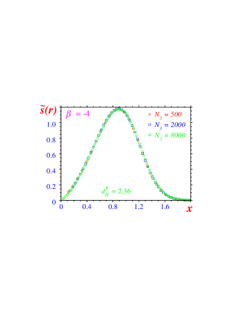
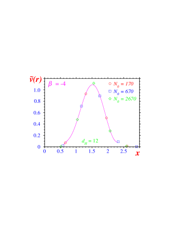
Figure 12: (Left) The simplex-simplex and (Right) the vertex-vertex distributions, $s(r)$ and $v(r)$, for $\beta=-4$ and $N_{3}=500$, 2000 and 8000. Both distributions are scaled according to Eq. (36) and are plotted vs. the scaling variable $x=r/N_{3}^{1/d_{H}}$. Notice, however, that different fractal dimensions, $d_{H}^{\prime}=2.36$ and $d_{H}=12$, are used in scaling the two distributions. The solid line is a polynomial interpolations.

Finally, we also determined the spectral dimension $d_{s}$ from the return probability of a random walker on the dual graph: $\rho(t)\sim t^{-d_{s}/2}$. The time $t$ is measured in units of jumps between neighboring simplexes, with a hopping probability $1/4$. These estimates of $d_{s}$, for volumes $N_{3}=500$, 2000, and 8000, are included in Figure 11. In the elongated phase we get $d_{s}\approx 4/3$, the value for a generic branched polymer, whereas in the crinkled phase the spectral dimension increases and reaches $d_{s}\approx 3/2$ for $\beta=-4$. Similar behavior is observed for the spectral dimension in $4D$ [9], although in that case the estimate in the crinkled phase was somewhat larger ($d_{s}\approx 1.8$ for $\beta=-3.5$). It is notable, however, that both in three and four dimensions the spectral dimension in the crinkled phase is less than two.

6 Conclusions

In this paper we have investigated an ensemble of maximal triangulations i.e. triangulations that, for a given volume are as close to the upper kinematic bound, $N_{0}/N_{D}=1/D$, as possible. This is motivated by the observation that this ensemble appears to reflect the properties of the weak-coupling limit of simplicial gravity, $\kappa_{0}\rightarrow\infty$.

In the first part of the paper, we presented an algorithm which, in the unmodified case $\beta=0$, yields an explicit enumeration of stacked spheres — a sub-class of the maximal ensemble. We also generalized this algorithm to include a modified measure, which, for $\beta\neq 0$, allows a recursive construction of a SCE of the corresponding partition function Eq. (6).

Using a combination of SCE and MC simulations, we investigated the properties of the maximal ensemble. We found that it is composed out of three distinct series, all with the same leading asymptotic behavior, but with different leading corrections $\gamma(k)$. This can be understood as the maximal ensemble includes, in addition to stacked spheres, triangulations that are “almost” stacked spheres, i.e. stacked spheres with one or two defects.

In the second part we demonstrated that with a suitable modified measure the maximal ensemble exhibits a transition to a crinkled phase, akin to what is observed in $4D$ simplicial gravity. This agrees with the phase diagram Figure 1. The scaling properties of this transition are consistent with a third order transition, i.e. with a specific heat exponent $\alpha=-1$. In the crinkled phase the intrinsic fractal structure is charcterized by a string susceptibility exponent $\gamma<0$, and Hausdorff dimension $d_{H}=\infty$ or $d_{H}^{\prime}\approx 2$, depending on whether it is measured on the triangulations, or its dual. This difference in the direct vs. dual fractal structure makes it unlikely that a thermodynamic limit exist in the crinkled phase, where a theory of extended manifolds emerges. The value of te spectral dimension measured on the dual graph agrees with the spectral dimension observed for the non–generic branched polymers. In the later case however exponent $\gamma$ is positive. In case of $\gamma<0$ BP model predicts $d_{s}=2$ [12]

We note the similarity between the above phase structure and what is observed in two dimensions if one varies the measure. There too is a soft continuous transition to a crumpled phase, for sufficiently negative $\beta$, where the string susceptibility exponent is negative [20] and the internal geometry collapses. Indeed, the similarity between $D=2$ and $D>2$ extends further. In both cases, the same phase strucuture is observed when sufficent amount of matter is coupled to the model. This can be understood, qualitativly, as the discretized form of the matter fields includes to a leading order the measure Eq. (6).

The phase diagram Figure 1 can also be partially understood from an analysis of a mean-field model which is related to branched polymers [21]. Restricted to the maximal ensemble this model predicts a soft (third order or greater) phase transition between an elongated and a crinkled phase. In a language of branched polymers this corresponds to a transition from an elongated (or a generic) phase with $\gamma=1/2$ and $d_{H}=2$, to a bush phase (non-generic) with $\gamma=1-\beta$ and $d_{H}=\infty$. The intrinsic crumpling in the bush phase is though much more pronounced than is observed in the crinkled phase of the maximal ensemble.

To which extend do we expect the maximal ensemble to correctly reflect the properties of the whole weak-coupling phase, $\kappa_{0}>\kappa_{0}^{c}$, of the model Eq. (2). In principle, this may depend on how one takes the two limits: the thermodynamic limit $N_{3}\rightarrow\infty$, and the weak-coupling limit $\kappa_{0}\rightarrow\infty$. A priori, these two limits need not commute. However, in Ref. [11] it is claimed that already for a finite $\kappa_{0}>\kappa_{0}^{c}$, the partition function Eq. (2) is dominated by triangulations which are close to stacked spheres.

Acknowledgments: G.T.  and P.B.  were supported by the Alexander von Humboldt Foundation.

Appendix A Enumerations of the maximal ensemble

In Tables 2 and 3 we list the first 20 terms in the SCE of both labeled and unlabeled staked spheres in three and four dimensions. The enumeration of unlabeled stacked spheres is given by the generating function Eq. (19), where:

$$h_{4}(t) = -\;{5\over 16}+\;{1\over 3}E_{1}\!\left(t\,E_{4}(t^{3})\right)-\;{1\over 6}E_{1}\!\left(t\,E_{4}(t^{3})\right)^{2}+\;{1\over 4}E_{2}\!\left(t\,E_{4}(t^{2})\right)$$

$$-\;{1\over 8}E_{2}\!\left(t\,E_{4}(t^{2})\right)^{2}+\;{1\over 6}E_{1}\!\left(t^{2}\,E_{4}(t^{6})\right)E_{2}\!\left(t^{3}\,E_{4}(t^{6})\right)+\;{1\over 24}E_{4}(t)$$

$$-\;{1\over 48}E_{4}(t)^{2}+\;{1\over 120}t\,E_{4}(t)^{5}+\;{1\over 12}t\,E_{2}\!\left(t\,E_{4}(t^{2})\right)^{3}E_{4}\!\left(t^{2}\right)+\;{1\over 8}t\,E_{4}\!\left(t^{2}\right)^{2}$$

$$+\;{13\over 48}t^{2}\,E_{4}\!\left(t^{2}\right)^{4}+\;{1\over 6}t\,E_{1}\!\left(t\,E_{4}(t^{3})\right)^{2}E_{4}\!\left(t^{3}\right)+\;{1\over 4}t\,E_{4}\!\left(t^{4}\right)$$

$$+\;{1\over 4}t^{2}\,E_{4}\!\left(t^{4}\right)^{2}+\;{1\over 5}t\,E_{4}\!\left(t^{5}\right)+\;{1\over 6}t^{2}\,E_{1}\!\left(t^{2}\,E_{4}(t^{6})\right)\,E_{4}\!\left(t^{6}\right)\,,$$

$$h_{5}(t) = -\;{19\over 60}+\;{1\over 8}E_{1}\!\bigl{(}t\,E_{5}(t^{2})^{2}\bigr{)}-\;{1\over 16}E_{1}\!\left(t\,E_{5}(t^{2})^{2}\right)^{2}+\;{1\over 4}E_{1}\!\left(t\,E_{5}(t^{4})\right)$$

$$-\;{1\over 8}E_{1}\!\left(t\,E_{5}(t^{4})\right)^{2}+\;{1\over 6}E_{2}\!\left(t\,E_{5}(t^{3})\right)-\;{1\over 12}E_{2}\!\left(t\,E_{5}(t^{3})\right)^{2}+\;{1\over 12}E_{3}\!\left(t\,E_{5}(t^{2})\right)$$

$$-\;{1\over 24}E_{3}\!\left(t\,E_{5}(t^{2})\right)^{2}+\;{1\over 6}\;t\,E_{2}\left(t^{2}\,E_{5}(t^{6})\right)\,E_{3}\left(t^{3}\,E_{5}(t^{6})\right)+\;{1\over 120}E_{5}(t)$$

$$+\;{1\over 12}\;t^{2}\,E_{2}\left(t^{2}\,E_{5}(t^{6})\right)^{2}\,E_{3}\left(t^{3}\,E_{5}(t^{6})\right)^{2}-\;{1\over 240}E_{5}(t)^{2}+\;{1\over 720}\;t\,E_{5}(t)^{6}$$

$$+\;{1\over 48}\;t\,E_{3}\left(t\,E_{5}(t^{2})\right)^{4}\,E_{5}\bigl{(}t^{2}\bigr{)}+\;{1\over 16}\;t\,E_{1}\left(t\,E_{5}(t^{2})^{2}\right)^{2}\;E_{5}\bigl{(}t^{2})^{2}$$

$$+\;{13\over 120}\,t^{2}\,E_{5}\bigl{(}t^{2}\bigr{)}^{5}+\;{1\over 18}\,t\,E_{2}\bigl{(}t\,E_{5}(t^{3})\bigr{)}^{3}\,E_{5}\bigl{(}t^{3}\bigr{)}+\;{1\over 18}\,t\,E_{5}\bigl{(}t^{3}\bigr{)}^{2}$$

$$+\;{1\over 8}\;t\,E_{1}\bigl{(}t\,E_{5}(t^{4})\bigr{)}^{2}\,E_{5}\bigl{(}t^{4}\bigr{)}+\;{1\over 8}\;t\,E_{1}\bigl{(}t^{2}\,E_{5}(t^{4})^{2}\bigr{)}\,E_{5}\bigl{(}t^{4}\bigr{)}+\;{1\over 48}\;t\,E_{5}\bigl{(}t^{2}\bigr{)}^{3}$$

$$+\;{1\over 8}\;t^{2}\,E_{1}\bigl{(}t^{2}\,E_{5}(t^{4})^{2}\bigr{)}\,E_{5}\bigl{(}t^{4}\bigr{)}+\;{1\over 5}\;t\,E_{5}\bigl{(}t^{5}\bigr{)}+\;{1\over 10}\;t^{2}\,E_{5}\bigl{(}t^{5}\bigr{)}^{2}$$

$$+\;{1\over 6}\;t\,E_{5}\bigl{(}t^{6}\bigr{)}+\;{1\over 6}\;t^{2}\,E_{2}\bigl{(}t^{2}\,E_{5}(t^{6})\bigr{)}^{2}\,E_{5}\bigl{(}t^{6}\bigr{)}+\;{1\over 10}\;t^{2}\,E_{5}\bigl{(}t^{10}\bigr{)}\,.$$

Table 2: The first 20 terms in the SCE of the both labeled and unlabeled three dimensional stacked spheres, $S^{0}(N_{3})$ and $h_{4,n}$, respectively. This is for $\beta=0$.

$n$	$\bigl{(}N_{0},N_{3}\bigr{)}$	$h_{4,n}$	$S^{0}(N_{3})$
1	(5,5)	1	1
2	(6,8)	1	5/2
3	(7,11)	1	10
4	(8,14)	3	50
5	(9,17)	7	285
6	(10,20)	30	1771
7	(11,23)	131	11700
8	(12,26)	795	80910
9	(13,29)	5152	579700
10	(14,32)	36800	8544965/2
11	(15,35)	272093	32224114
12	(16,38)	2077909	247754390
13	(17,41)	16176607	1936016950
14	(18,44)	127996683	15340200750
15	(19,47)	1025727646	123020557800
16	(20,50)	8310377720	996993749142
17	(21,53)	67967600763	8155209690540
18	(22,56)	560527576100	67259885983090
19	(23,59)	4656993996246	558826638901000
20	(24,62)	38949328897318	4673871155753800

Table 3: Same as Table 2, except for four dimensional stacked spheres.

$n$	$\bigl{(}N_{0},N_{4}\bigr{)}$	$h_{5,n}$	$S^{0}(N_{4})$
1	(6,6)	1	1
2	(7,10)	1	3
3	(8,14)	1	15
4	(9,18)	3	95
5	(10,22)	7	690
6	(11,26)	30	5481
7	(12,30)	142	46376
8	(13,34)	922	411255
9	(14,38)	6848	3781635
10	(15,42)	57994	35791910
11	(16,46)	525048	346821930
12	(17,50)	4999697	3427001253
13	(18,54)	49159506	34425730640
14	(19,58)	494873071	350732771160
15	(20,62)	5068890252	3617153918640
16	(21,66)	52632367550	37703805776935
17	(22,70)	552579655767	396716804816265
18	(23,74)	5855580019967	4209161209968825
19	(24,78)	62548009026369	44993046668984145
20	(25,82)	672818970206219	484176486362971710

The values in Tables 2 and 3 can be compared to Table 8 of Ref. [13]. Although for most volumes they agree there are few discrepancies. We have, however, an independent confirmation on our calculations; for $N_{D}\leq 38$ we have explicitly identified all distinct triangulations.

Figure 13: The successibe ratios, $s_{n}^{-1}=S_{n}/S_{n-1}$, for the sequence of labeled vs. unlabeled stacked spheres. The arrow indicates the correct asymptotic value $z^{-1}=256/27$. For unlabeled triangulations the irregular behavior is due to non-analytic corrections.

As discussed in Section 4.1, although the leading asymptotic behavior is identical for the ensemble of labeled vs. unlabeled stacked spheres, for the latter the sub-leading corrections are non-analytic. This effect, which is demonstrated in Figure (13), makes it virtually impossible to extract the asymptotic behavior of unlabeled triangulations using series extrapolation methods.

In Table 4 we list the first 10 and 8 terms of two non-minimal series, $S^{1}$ and $S^{2}$, calculated by directly identifying all distinct triangulations in MC simulations.

Table 4: The first few terms in the SCE of the $3D$ maximal ensemble for the two non-minimal series $S^{1}$ and $S^{2}$. $n_{k}$ is the number of distinct (unlabeled) triangulations.

$N_{0}$	$N_{3}$	$n_{1}$	$S^{1}(N_{3})$	$N_{3}$	$n_{2}$	$S^{2}(N_{3})$
6	9	1	5/3
7	12	2	35/2	13	1	15
8	15	5	152	16	8	4205/16
9	18	23	3800/3	19	45	3290
10	21	124	73370/7	22	385	72535/2
11	24	859	348075/4	25	3435	375750
12	27	6518	6544720/9	28	32710	15043835/4
13	30	52761	6121632	31	312601	36867985
14	33	438954	570959025/11	34	2995589	713253255/2
15	36	3717370	886163135/2

Appendix B The contact term

As discussed in Section 5.2, for minbu’s on maximal triangulations, the interactions at neck — the contact term — play a (unusually) big and non-trivial role in the crinkled phase. It is essential to take these interactions into account when estimating $\gamma$ from a fit to the measured minbu distributions. In this appendix we analyze the behavior of the contact term and explain why it plays such an important role for this particular ensemble.

In the nomenclature of Section 3 we can write the minbu distribution, Eq. (33), for $\beta=0$ and measured on a stacked sphere of size $n$, as

$${\cal B}_{n}(b)\;\propto\;\frac{e_{4,b}\,e_{4,n-b}}{e_{4,n}}\;\propto\;\bigl{(}3(n\!-\!b)+2\bigr{)}\bigl{(}3b+2\bigr{)}\;\frac{W_{3}(b)W_{3}(n-b)}{W_{3}(n)}$$

However, for $\beta\neq 0$ the situation is different. We must take into account the different possible distributions of vertex orders, ${\bf p}$ and ${\bf q}$, on the marked simplex (the neck), both on the baby and on the mother. The distribution is then

$$\widetilde{\cal B}_{n}(b;\beta)\;\propto\;\frac{1}{W_{3}(n)}\;\sum_{{\bf p},{\bf q}}\;\;\prod_{i=1}^{4}\;(p_{i}+q_{i}-2)^{\beta}\;e({\bf p};n\!-\!b,\beta)\;e({\bf q};b,\beta)\;.$$ (39)

Defining

$$w(\mathbf{q};n,\beta)\;=\;\frac{e(\mathbf{q};n,\beta)}{e(n,\beta)}\,\prod_{i=1}^{4}q_{i}^{\beta}\;,$$ (40)

we can rewrite Eq. (39) as

$$\widetilde{\cal B}_{n}(b;\beta) \propto \bigl{(}3(n-b)+2\bigr{)}\bigl{(}3b+2\bigr{)}\,\frac{W_{3}(b)\;W_{3}(n\!-\!b)}{W_{3}(n)}$$ (41)

$$\;\;\;\;\times\sum_{{\bf q},{\bf p}}\;w({\bf q};n\!-\!b,\beta)\,w({\bf p};b,\beta)\,\prod_{i=1}^{4}\frac{(q_{i}+p_{i}-2)^{\beta}}{q_{i}^{\beta}p_{i}^{\beta}}$$

$$\equiv {\cal B}_{n}(b;\beta)\cdot{\cal C}_{n}(b;\beta)\;,$$

where we define ${\cal C}_{n}(b;\beta)$ as the contact term..

The following argument gives some idea of the relevance of the contact term in the different phases. If we assume that the distribution $w({\bf q})$ factorizes,

$$w({\bf q};n,\beta)\;=\;\prod_{i=1}^{4}\,w(q_{i};n,\beta)\;,$$ (42)

then the distribution $w(q;n)$ is related to the vertex order distribution $\pi(q)$, i.e. the probability of finding a vertex with given order $q$, through

$$w(q;n,\beta)\;=\;\frac{q\,\pi(q;n,\beta)}{\langle q\rangle}.$$ (43)

In the elongated phase the distribution $w(q;n)$ decays exponentially, whereas in the crinkled phase vertices of large order are favored and the distribution has a power-law decay (Figure 8).

An exponential decay of $w(q;n)$ effectively introduces a cut-off in the sum over vertex orders in Eq. (41). Hence, for sufficiently large triangulations the contact term becomes independent of the volume. In contrast, in the crinkled phase there is no such cut-off and we can expect a strong volume dependence. This is demonstrated by numerical measurements of the contact term, shown in Figure 14. In the elongated phase, $\beta=2$, the contact term ${\cal C}_{n}(2)$ is more or less constant for $\beta\gtrsim 50$, whereas for $\beta=-4$ the contact term $C_{n}(-4)$ depends strongly on $b$.

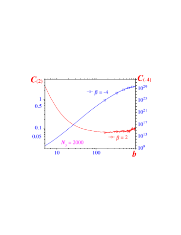
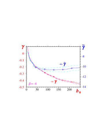
Figure 14: (Left) The dependence of the contact term, ${\cal C}_{n}(b;\beta)$, on the minbu size $b$. This is for $N_{3}=2000$ and both in the elongated phase, $\beta=2$, and in the crinkled phase, $\beta=-4$: $C(2)$ and $C(-4)$. (Right) The exponent $\gamma$, determined by a fit to the minbu distribution Eq. (33) for $N_{3}=2000$ and $\beta=-4$. Results are shown varying a lower cut-off $b_{0}$ in the fit, and both with and without the contact term divided out, $\widetilde{\gamma}$ and $\gamma$ respectively. Note that in both plots the compared curves are plotted on very different scales.

Although this effect can be expected for any ensemble modified by the measure Eq. (6), the particular construction of maximal triangulations, by a repeated application of move $\left(1,4\right)$, enhances the role of the contact term. For every time move $\left(1,4\right)$ is applied one minimal neck is generated, hence for a maximal triangulation the number of minbu’s is fixed. Thus the minbu distributions, measured on $S^{0}$, is more constrained than measured on a general ensemble where triangulations with fewer minbu’s are favored as $\beta\rightarrow\infty$.

How does all this affect the measurements of $\gamma\;$? The standard method for extracting $\gamma$ from a minbu distribution is to impose a lower cut-off $b_{0}$ on the minbu size included in the fit to Eq. (33). The cut-off is then increased until a stable estimate of $\gamma(b_{0})$ is obtained [22]. In the elongated phase, and in general for most models of simplicial gravity, this methods works fine. However, for stacked spheres this method fails in the crinkled phase. Unless the contact term is eliminated, i.e. divided out of the minbu distribution in the measurement process, a stable plateau in $\gamma(b_{0})$ is not observed. An example of this is shown in Figure 14 for $\beta=-4$.

References

- [1]
-
[2]
J. Ambjørn, B. Durhuus, J. Fröhlich, P. Orland,
Nucl. Phys. B 257 (1985) 433; B 270 (1986) 457; B 275 (1986) 161;
F. David, Nucl. Phys B 257 (1985) 543.
V.A Kazakov, I. Kostov, A.A Migdal, Phys. Lett. B157 (1985) 295; Nucl. Phys. B 275 (1986) 641. -
[3]
J. Ambjørn, B. Durhuus, T. Jonsson, Mod. Phys. Lett. A 6 (1991) 1133.
M.E. Agishtein, A.A Migdal, Mod. Phys. Lett. A 6 (1991) 1863. -
[4]
B. Boulatov, A. Krzywicki, Mod. Phys. Lett. A 6 (1991) 3005.
J. Ambjørn, S. Varsted, Nucl. Phys. B 373 (1992) 557. -
[5]
F. David, Simplicial Quantum Gravity and Random
Lattices, (hep-th/9303127), Lectures given at Les
Houches Summer School on Gravitation and Quantizations,
Session LVII, Les Houches, France, 1992;
J. Ambjørn, B. Durhuus and T. Jonsson,
Quantum Geometry: A statistical field theory approach,
Cambridge University Press, 1997;
G. Thorleifsson, Lattice Gravity and Random Surfaces, review talk at LATTICE 98, (hep-th/9809131. - [6] P. Pialas, Z. Burda, A. Krzywicki and B. Petersson, Nucl. Phys. B 472 (1996) 293.
-
[7]
B. Brugmann and E. Marinari,
Phys. Rev. Lett. 70 (1993) 1908;
S. Catterall, J. Kogut and R. Renken, Phys. Lett. B 342 (1995) 53; Nucl. Phys. B 523 (1998) 553;
T. Hotta, T. Izubuchi and J. Nishimura, Nucl. Phys. B 531 (1998) 446. -
[8]
R.L. Renken, S.M. Catterall and J. Kogut,
Nucl. Phys. B 422 (1994) 677;
J. Ambjørn, J. Jurkiewicz, S. Bilke, Z. Burda and B. Petersson, Mod. Phys. Lett. A 9 (1994) 2527;
J. Ambjorn, Z. Burda, J. Jurkiewicz and C.F. Kristjansen, Phys. Lett. B 297 (1992) 253. - [9] S. Bilke, Z. Burda, A. Krzywicki, B. Petersson, J. Tabaczek and G. Thorleifsson, Phys. Lett. B 418 (1998) 266; Phys. Lett. B 432 (1998) 279.
- [10] M. Gross and S. Varsted, Nucl. Phys. B 378 (1992) 367.
-
[11]
J. Ambjørn, M. Carfora and A. Marzuoli,
The Geometry of Dynamical Triangulations,
Lectures Notes in Phys. 50, Springer-Verlag, 1997;
D. Gabrielli, Phys. Lett. B 421 (1998) 79. - [12] D. Walkup, Acta Math. 125 75.
- [13] F. Hering, R.C. Read and G.C. Shephard, Discrete Math4̇0 (1982) 203.
- [14] J. Riordan, Combinatorial identities (Wiley, New York, 1968).
- [15] A.J. Guttmann, Asymprotica Analysis of Power Seris Expansions, in: C. Domb and J. Lebowitz (eds) Phase Transitions and Critical Phenomena, Vol. 13, (Academic, New York, 1989).
- [16] S. Jain and S.D. Mathur, Phys. Lett. B 286 (1992) 239.
- [17] S. Bilke and G. Thorleifsson, Simulating Four-Dimensional Simplicial Gravity using Degenerate Triangulations, (hep-lat/9810049).
- [18] D.J. Gross, I.Klebanov, Nucl. Phys. B 344 (1990) 475.
-
[19]
S. Catterall, G. Thorleifsson, M. Bowick and V. John,
Phys. Lett. B 354 (1995) 56;
J. Ambjørn, J. Jurkiewicz and Y. Watabiki, Nucl. Phys. B 454 (1995) 313. - [20] J. Ambjørn, B. Durhuus and J. Frolich, Nucl. Phys. B 275 (1986) 161.
-
[21]
P. Bialas, Z. Burda, Phys. Lett. B 384 (1996) 75.
P. Bialas, Z. Burda, D. Johnston, Nucl. Phys. B 493 (1997) 505
P. Bialas, Z. Burda, D. Johnston, “Phase diagram of the mean field model of simplicial gravity” gr-qc/9808011 to be published in Nucl. Phys. B -
[22]
J. Ambjørn, S. Jain and G. Thorleifsson,
Phys. Lett. B 307 (1993) 34;
J. Ambjørn and G. Thorleifsson, Phys. Lett. B 323 (1994) 7. - [23]