Matrix elements relevant for $\Delta I=1/2$ rule and $\varepsilon^{\prime}/\varepsilon$ from Lattice QCD with staggered fermions

We perform a study of matrix elements relevant for the $\Delta I=1/2$ rule and the direct CP-violation parameter $\varepsilon^{\prime}/\varepsilon$ from first principles by computer simulation in Lattice QCD. We use staggered (Kogut-Susskind) fermions, and employ the chiral perturbation theory method for studying $K^{0}\to\pi\pi$ decays. Having obtained a reasonable statistical accuracy, we observe an enhancement of the $\Delta I=1/2$ amplitude, consistent with experiment within our large systematic errors. Finite volume and quenching effects have been studied and were found small compared to noise. The estimates of $\varepsilon^{\prime}/\varepsilon$ are hindered by large uncertainties associated with operator matching. In this paper we explain the simulation method, present the results and address the systematic uncertainties.

1 Introduction

In those areas of particle phenomenology which require addressing non-perturbative effects, Lattice QCD plays an increasingly significant role, being a first-principles method. The rapid advances in computational performance as well as algorithmic techniques are allowing for better control of various errors associated with lattice calculations.

In this paper we address the phenomenology of $K^{0}\to\pi\pi$ decays. One of the long-standing puzzles is the “$\Delta I=1/2$ rule”, which is the observation that the transition channel with isospin changing by 1/2 is enhanced 22 times with respect to transitions with isospin changing by 3/2. The strong interactions are essential for explaining this effect within the Standard Model. Since the energy scales involved in these decays are rather small, computations in quantum chromodynamics (QCD) have to be done using a non-perturbative method such as Lattice QCD. Namely, Lattice QCD is used to calculate hadronic matrix elements of the operators appearing in the effective weak Hamiltonian.

There have been so far several other attempts to study matrix elements of the operators relevant for $\Delta I=1/2$ rule on the lattice [3, 4, 6], but they fell short of desired accuracy. In addition, several groups [7, 5] have studied matrix elements $\langle\pi^{+}\pi^{0}|O_{i}|K^{+}\rangle$, which describe only $\Delta I=3/2$, not $\Delta I=1/2$ transition. In the present simulation, the statistics is finally under control for $\Delta I=1/2$ amplitude.

Our main work is in calculating matrix elements $\langle\pi^{+}|O_{i}|K^{+}\rangle$ and $\langle 0|O_{i}|K^{0}\rangle$ for all basis operators (introduced in Sec. 2.1). This is enough to recover matrix elements $\langle\pi\pi|O_{i}|K^{0}\rangle$ using chiral perturbation theory in the lowest order, although this procedure suffers from uncertainties arising from ignoring higher orders (in particular, final state interactions). The latter matrix elements are an essential part of the phenomenological expressions for $\Delta I=1/2$ and $\Delta I=3/2$ amplitudes, as well as $\varepsilon^{\prime}/\varepsilon$. The ratio of the amplitudes computed in this way confirms significant enhancement of $\Delta I=1/2$ channel, although systematic uncertainties preclude a definite answer.

In addition, we address a related issue of $\varepsilon^{\prime}/\varepsilon$ – the direct CP-violation parameter in the neutral kaon system. As of the day of writing, the experimental data are somewhat ambiguous about this parameter: the group at CERN (NA48) [1] reports $\mbox{Re}(\varepsilon^{\prime}/\varepsilon)=\mbox{ $(23\pm 7)\times 10^{-4},$}$ while the Fermilab group (E731) [2] has found $\mbox{Re}(\varepsilon^{\prime}/\varepsilon)=\mbox{$(7.4\pm 6.0)\times 10^{-4}$.}$ There is a hope that the discrepancy between the two reports will soon be removed in a new generation of experiments.

On the theoretical side, the progress in estimating $\varepsilon^{\prime}/\varepsilon$ in the Standard Model is largely slowed down by the unknown matrix elements [12] of the appropriate operators. The previous attempts [3, 4, 6] to compute them on the lattice did not take into account operator matching. In this work we repeat this calculation with better statistics and better investigation of systematic uncertainties. We are using perturbative operator matching. In some cases it does not work, so we explore alternatives and come up with a partially non-perturbative renormalization procedure. The associated errors are estimated to be large. This is currently the biggest stumbling block in computing $\varepsilon^{\prime}/\varepsilon$.

The paper is structured as follows. In the Section 2 we show the context of our calculations, define the quantities we are looking after and discuss a number of theoretical points relevant for the calculation. Section 3 discusses issues pertaining to the lattice simulation. In Section 4 we present the results and discuss systematic errors for $\Delta I=1/2$ rule amplitudes. In Section 5 we explain how the operator matching problem together with other systematic errors preclude a reliable calculation of $\varepsilon^{\prime}/\varepsilon$, and give our best estimates for this quantity in Section 6. Section 7 contains the conclusion. In the Appendix we give details about the quark operators and sources, and provide explicit expressions for all contractions and matrix elements for reference purposes.

2 Theoretical framework

2.1 Framework and definitions

The standard approach to describe the problems in question is to use the Operator Product Expansion at the $M_{W}$ scale and use the Renormalization Group equations to translate the effective weak theory to more convenient scales ($\mu\sim$ 2–4 GeV). At these scales the effective Hamiltonian for $K\to\pi\pi$ decays is the following linear superposition [12]:

$$H_{\mathrm{W}}^{\mathrm{e}ff}=\frac{G_{F}}{\sqrt{2}}V_{ud}\,V^{*}_{us}\sum_{i=1}^{10}\Bigl{[}z_{i}(\mu)+\tau y_{i}(\mu)\Bigr{]}O_{i}(\mu)\,,$$ (1)

where $z_{i}$ and $y_{i}$ are Wilson coefficients (currently known at two-loop order), $\tau\equiv-V_{td}V_{ts}^{*}/V_{ud}V_{us}^{*}$, and $O_{i}$ are basis of four-fermions operators defined as follows:

$$O_{1} = (\bar{s}_{\alpha}\gamma_{\mu}(1-\gamma_{5})u_{\beta})(\bar{u}_{\beta}\gamma^{\mu}(1-\gamma_{5})d_{\alpha})$$ (2)

$$O_{2} = (\bar{s}_{\alpha}\gamma_{\mu}(1-\gamma_{5})u_{\alpha})(\bar{u}_{\beta}\gamma^{\mu}(1-\gamma_{5})d_{\beta})$$ (3)

$$O_{3} = (\bar{s}_{\alpha}\gamma_{\mu}(1-\gamma_{5})d_{\alpha})\sum_{q}(\bar{q}_{\beta}\gamma^{\mu}(1-\gamma_{5})q_{\beta})$$ (4)

$$O_{4} = (\bar{s}_{\alpha}\gamma_{\mu}(1-\gamma_{5})d_{\beta})\sum_{q}(\bar{q}_{\beta}\gamma^{\mu}(1-\gamma_{5})q_{\alpha})$$ (5)

$$O_{5} = (\bar{s}_{\alpha}\gamma_{\mu}(1-\gamma_{5})d_{\alpha})\sum_{q}(\bar{q}_{\beta}\gamma^{\mu}(1+\gamma_{5})q_{\beta})$$ (6)

$$O_{6} = (\bar{s}_{\alpha}\gamma_{\mu}(1-\gamma_{5})d_{\beta})\sum_{q}(\bar{q}_{\beta}\gamma^{\mu}(1+\gamma_{5})q_{\alpha})$$ (7)

$$O_{7} = \frac{3}{2}(\bar{s}_{\alpha}\gamma_{\mu}(1-\gamma_{5})d_{\alpha})\sum_{q}e_{q}(\bar{q}_{\beta}\gamma^{\mu}(1+\gamma_{5})q_{\beta})$$ (8)

$$O_{8} = \frac{3}{2}(\bar{s}_{\alpha}\gamma_{\mu}(1-\gamma_{5})d_{\beta})\sum_{q}e_{q}(\bar{q}_{\beta}\gamma^{\mu}(1+\gamma_{5})q_{\alpha})$$ (9)

$$O_{9} = \frac{3}{2}(\bar{s}_{\alpha}\gamma_{\mu}(1-\gamma_{5})d_{\alpha})\sum_{q}e_{q}(\bar{q}_{\beta}\gamma^{\mu}(1-\gamma_{5})q_{\beta})$$ (10)

$$O_{10} = \frac{3}{2}(\bar{s}_{\alpha}\gamma_{\mu}(1-\gamma_{5})d_{\beta})\sum_{q}e_{q}(\bar{q}_{\beta}\gamma^{\mu}(1-\gamma_{5})q_{\alpha})$$ (11)

Here $\alpha$ and $\beta$ are color indices, $e_{q}$ is quark electric charge, and summation is done over all light quarks.

Isospin amplitudes are defined as

$$A_{0,2}e^{i\delta_{0,2}}\equiv\langle(\pi\pi)_{I=0,2}|H_{W}|K^{0}\rangle,$$ (12)

where $\delta_{0,2}$ are the final state interaction phases of the two channels. Experimentally

$$\omega=\mbox{Re}A_{0}/\mbox{Re}A_{2}\simeq 22\,.$$ (13)

Direct CP violation parameter $\varepsilon^{\prime}$ is defined in terms of imaginary parts of these amplitudes:

$$\varepsilon^{\prime}=-\frac{\mbox{Im}A_{0}-\omega\mbox{Im}A_{2}}{\sqrt{2}\omega\mbox{Re}A_{0}}e^{i(\pi/2+\delta_{2}-\delta_{0})}.$$ (14)

Experiments are measuring the quantity $\mbox{Re}\varepsilon^{\prime}/\varepsilon$, which is given by

$$\mbox{Re}\,\frac{\varepsilon^{\prime}}{\varepsilon}\simeq\frac{G_{F}}{2\omega|\varepsilon|\mbox{Re}{A_{0}}}\,\mbox{Im}\,\lambda_{t}\,\,\left[\Pi_{0}-\omega\>\Pi_{2}\right],$$ (15)

where

$$\Pi_{0} = \sum_{i}y_{i}\,\langle(\pi\pi)_{I=0}|O_{i}^{(0)}|K^{0}\rangle(1-\Omega_{\eta+\eta^{\prime}})$$ (16)

$$\Pi_{2} = \sum_{i}y_{i}\,\langle(\pi\pi)_{I=2}|O_{i}^{(2)}|K^{0}\rangle$$ (17)

with $\mbox{Im}\,\lambda_{t}\equiv\mbox{Im}V_{td}V^{*}_{ts}$, and where $\Omega_{\eta+\eta^{\prime}}\sim 0.25\pm 0.05$ takes into account the effect of isospin breaking in quark masses ($m_{u}\neq m_{d}$). $O_{i}^{(0)}$ and $O_{i}^{(2)}$ are isospin 0 and 2 parts of the basis operators. Their expressions are given in the Appendix for completeness.

2.2 Treatment of charm quark

The effective Hamiltonian given above is obtained in the continuum theory in which the top, bottom and charm quarks are integrated out. (In particular, the summation in Eqs. (4–11) is done over $u$, $d$ and $s$ quarks.) This makes sense only when the scale $\mu$ is sufficiently low compared to the charm quark mass. As mentioned in Ref. [8], at scales comparable to $m_{c}$ higher-dimensional operators can contribute considerably. Then one should consider an expanded set of operators including those containing the charm quark. Lattice treatment of the charm quark is possible but in practice quite limited, for example by having to work at much smaller lattice spacings and having a more complicated set of operators and contractions. Therefore we have opted to work in the effective theory in which the charm quark is integrated out. Since we typically use $\mu\sim 2$ GeV in our simulations, this falls into a dangerous region. We hope that the effects of higher-dimensional operators can still be neglected, but strictly speaking this issue should be separately investigated.

2.3 Calculating $\langle\pi\pi|O_{i}|K^{0}\rangle$.

As was shown by Martinelli and Testa [14], two-particle hadronic states are very difficult to construct on the lattice (and in general, in any Euclidean description). We have to use an alternative procedure to calculate the matrix elements appearing in Eqs. (12,16,17). We choose the method  [11] in which the lowest-order chiral perturbation theory is used to relate $\langle\pi\pi|O_{i}|K^{0}\rangle$ to matrix elements involving one-particle states:

$$\langle\pi^{+}\pi^{-}|O_{i}|K^{0}\rangle = \frac{m_{K}^{2}-m_{\pi}^{2}}{f}\gamma$$ (18)

$$\langle\pi^{+}|O_{i}|K^{+}\rangle = (p_{\pi}\cdot p_{K})\gamma-\frac{m_{s}+m_{d}}{f}\delta$$ (19)

$$\langle 0|O_{i}|K^{0}\rangle = (m_{s}-m_{d})\delta,$$ (20)

where $f$ is the lowest-order pseudoscalar decay constant. The masses in the first of these formulae are the physical meson masses, while the quark masses and the momenta in the second and third formulae are meant to be from actual simulations on the lattice (done with unphysical masses). These relationships ignore higher order terms in the chiral expansion, most importantly the final state interactions. Therefore this method suffers from a significant uncertainty. Golterman and Leung [18] have computed one-loop correction for $\Delta I=3/2$ amplitude in chiral perturbation theory. They find this correction can be large, up to 30% or 60%, depending on the values of unknown contact terms and the cut-off.

3 Lattice techniques

3.1 Mixing with lower-dimensional operators.

Eqs. (18–20) handle unphysical $s\leftrightarrow d$ mixing in $\langle\pi^{+}|O_{i}|K^{+}\rangle$ by subtracting the unphysical part proportional to $\langle 0|O_{i}|K^{0}\rangle$. This is equivalent to subtracting the operator

$$O_{sub}\equiv(m_{d}+m_{s})\bar{s}d+(m_{d}-m_{s})\bar{s}\gamma_{5}d\,.$$ (21)

As shown by Kilcup, Sharpe et al. in Refs. [9, 10], these statements are also true on the lattice if one uses staggered fermions. A number of Ward identities discussed in these references show that lattice formulation with staggered fermions retains the essential chiral properties of the continuum theory. In particular, $O_{sub}$ defined in Eq. 21 is the only lower-dimensional operator appears in mixing with the basis operators. (Lower-dimensional operators have to be subtracted non-perturbatively since they are multiplied by powers of $a^{-1}$.) We employ the non-perturbative procedure suggested in Ref. [10]:

$$\langle\pi^{+}\pi^{-}|O_{i}|K^{0}\rangle=\langle\pi^{+}|O_{i}-\alpha_{i}O_{sub}|K^{+}\rangle\cdot\frac{m_{K}^{2}-m_{\pi}^{2}}{(p_{\pi}\cdot p_{K})f}\,,$$ (22)

where $\alpha_{i}$ are found from

$$0=\langle 0|O_{i}-\alpha_{i}O_{sub}|K^{0}\rangle\,.$$ (23)

This procedure is equivalent to the lattice version of Eqs. (18–20) and allows subtraction timeslice by timeslice.

Throughout our simulation we use only degenerate mesons, i.e. $m_{s}=m_{d}=m_{u}$. Since only negative parity part of $O_{sub}$ contributes in Eq. (23), one naively expects infinity when calculating $\alpha_{i}$. However, matrix elements $\langle 0|O_{i}|K^{0}\rangle$ of all basis operators vanish when $m_{s}=m_{d}$ due to invariance of both the Lagrangian and all the operators in question under the CPS symmetry, which is defined as the CP symmetry combined with interchange of $s$ and $d$ quarks. Thus calculation of $\alpha_{i}$ requires taking the first derivative of $\langle 0|O_{i}|K^{0}\rangle$ with respect to $(m_{d}-m_{s})$. In order to evaluate the first derivative numerically, we insert another fermion matrix inversion in turn into all propagators involving the strange quark. Detailed expressions for all contractions are given in the Appendix.

Figure 1: Five diagrams types needed to be computed: (a) “Eight”; (b) “Eye”; (c) “Annihilation”; (d) “Subtraction”; (e) two-point function.

3.2 Diagrams to be computed

According to Eqs. (22,23), we need to compute three diagrams involving four-fermion operators (shown in Fig. 1) and a couple of bilinear contractions. The “eight” contraction type (Fig. 1a) is relatively cheap to compute. It is the only contraction needed for the $\Delta I=3/2$ amplitude. The “eye” and “annihilation” diagrams (Fig. 1b and 1c) are much more expensive since they involve calculation of propagators from every point in space-time.

3.3 Lattice parameters and other details

The parameters of simulation are listed in the Table 1. We use periodic boundary conditions in both space and time. Our main “reference” ensemble is a set of quenched configurations at $\beta\equiv 6/g^{2}=6.0$ ($Q_{1}$). In addition, we use an ensemble with a larger lattice volume ($Q_{2}$), an ensemble with $\beta=6.2$ ($Q_{3}$) for checking the lattice spacing dependence, and an ensemble with 2 dynamical flavors ($m=0.01$) generated by the Columbia group, used for checking the impact of quenching. The ensembles were obtained using 4 sweeps of $SU(2)$ overrelaxed and 1 sweep of $SU(2)$ heatbath algorithm. The configurations were separated by 1000 sweeps, where one sweep includes three $SU(2)$ subgroups updates.

Table 1: Simulation parameters

Ensemble	$N_{f}$	$\beta$	Size	L, fm	Number of	Quark masses
name					configurations	used
$Q_{1}$	0	6.0	$16^{3}\times(32\times 4)$	1.6	216	0.01 — 0.05
$Q_{2}$	0	6.0	$32^{3}\times(64\times 2)$	3.2	26	0.01 — 0.05
$Q_{3}$	0	6.2	$24^{3}\times(48\times 4)$	1.7	26	0.005 — 0.03
$D$	2	5.7	$16^{3}\times(32\times 4)$	1.6	83	0.01 — 0.05

We use the standard staggered fermion action. Fermion matrices are inverted by conjugate gradient. Jackknife is used for statistical analysis.

As explained below, we have extended the lattice 4 times in time dimension by copying gauge links. This is done in order to get rid of excited states contamination and wrap-around effects.

The lattice spacing values for quenched ensembles were obtained by performing a fit in the form of the asymptotic scaling to the quenched data of $\rho$ meson mass given elsewhere [17]. Lattice spacing for the dynamical ensemble is also set by the $\rho$ mass [16].

Some other technicalities are as follows. We work in the two flavor formalism. We use local wall sources that create pseudoscalar mesons at rest. (Smearing did not have a substantial effect.) The mesons are degenerate ($m_{s}=m_{d}=m_{u}$, $m_{\pi}=m_{K}$). We use staggered fermions and work with gauge-invariant operators, since the gauge symmetry enables significant reduction of the list of possible mixing operators. The staggered flavour structure is assigned depending on the contraction type. Our operators are tadpole-improved. This serves to ‘improve” the perturbative expansion at a later stage when we match the lattice and continuum operators. For calculating fermion loops we employ the $U(1)$ pseudofermion stochastic estimator. More details and explanation of some of these terms can be found in the Appendix.

Figure 2: The general setup of calculation of $\langle\pi^{+}|O_{i}|K^{+}\rangle$ (without loss of generality, an “eight” contraction is shown). The kaon source is at the timeslice 0, while the pion sink is at the timeslice $T$. The operator is inserted at a variable time $t$. The result of this contraction is proportional to the product of two exponentials shown in the figure.

3.4 Setup for calculating matrix elements of four-fermion
operators

Consider the setup for calculation of $\langle\pi^{+}|O_{i}|K^{+}\rangle$. Kaons are created at $t_{0}=0$, the operators are inserted at a variable time $t$, and the pion sink is located at the time $T$ (see Fig. 2), where $T$ is sufficiently large. In principle, a number of states with pseudoscalar quantum numbers can be created by the kaon source. Each state’s contribution is proportional to $\sqrt{Z}e^{-m|t|}$, so the lightest state (kaon) dominates at large enough $t$. Analogously, states annihilated by the sink contribute proportionally to $\sqrt{Z}e^{-m|T-t|}$, which is dominated by the pion.

In this work kaon and pion have equal mass. In the middle of the lattice, where $t$ is far enough from both 0 and $T$, we expect to see a plateau, corresponding to $Ze^{-m_{\pi}T}\langle\pi|O|K\rangle$. This plateau is our working region (see Fig. 4).

As concerns the kaon annihilation matrix elements $\langle 0|O_{i}|K^{0}\rangle$, we only need their ratio to $\langle 0|\overline{s}\gamma_{5}d|K^{0}\rangle$, in which the factors $\sqrt{Z}e^{-mt}$ cancel. Indeed, we observe a rather steady plateau (Fig. 5).

Figure 3: $B$ ratio is formed by dividing the four-fermion matrix element by the product of two-point functions, typically involving $A_{\mu}$ or $P$ bilinears. All the operators involved are inserted at the same timeslice $t$, and summation is done over spatial volume. The external meson sources are located at timeslices 0 and $T$, both in the numerator and the denominator. This enables cancellation of some common factors.

3.5 $B$ ratios

It has become conventional to express the results for matrix elements in terms of so-called $B$ ratios, which are the ratios of desired four-fermion matrix elements to their values obtained by vacuum saturation approximation (VSA). For example, the $B$ ratios of operators $O_{2}$ and $O_{4}$ are formed by dividing the full matrix element by the product of axial-current two-point functions (Fig. 3). We expect the denominator to form a plateau in the middle of the lattice, equal to $Ze^{-m_{\pi}T}\,\langle\pi|A_{\mu}|0\rangle\,\cdot\,\langle 0|A^{\mu}|K\rangle$, where $A^{\mu}$ are the axial vector currents with appropriate flavor quantum numbers for kaon and pion. The factor $Ze^{-m_{\pi}T}$ cancels, leaving the desirable ratio $\langle\pi|O|K\rangle\,/\,(\langle\pi|A_{\mu}|0\rangle\,\cdot\,\langle 0|A^{\mu}|K\rangle)$. Apart from common normalization factors, a number of systematic uncertainties also tend to cancel in this ratio, including the uncertainty in the lattice spacing, quenching and in some cases perturbative correction uncertainty. Therefore, it is sometimes reasonable to give lattice answers in terms of the $B$ ratios.

However, eventually the physical matrix element needs to be reconstructed by using the known experimental parameters (namely $f_{K}$) to compute VSA. In some cases, such as for operators $O_{5}$—$O_{8}$, the VSA itself is known very imprecisely due to the failure of perturbative matching (see Sec. 5). Then it is more reasonable to give answers in terms of matrix elements in physical units. We have adopted the strategy of expressing all matrix elements in units of $\langle\pi|A_{\mu}|0\rangle\,\langle 0|A^{\mu}|K\rangle=(f_{K}^{latt})^{2}m_{M}^{2}$ at an intermediate stage, and using pre-computed $f_{K}^{latt}$ at the given meson mass to convert to physical units. This method is sensitive to the choice of the lattice spacing.

Figure 4: An example of the signal we get for one of the $B$ ratios (in this case, for the “eye” part of the $O_{2}$ operator on $Q_{1}$ ensemble). The wall sources are at $t=1$ and $t=49$. We see that the excited states quickly disappear and a stable, well-distinguished plateau is observed. We perform jackknife averaging in the range of $t$ from 12 to 37 (shown with the horizontal lines). It is important to confirm the existence of the plateau for reliability of the results.

Figure 5: An example of the signal for $\langle 0|O_{2}|K^{0}\rangle\,/\,[(m_{d}-m_{s})\,\langle 0|\overline{s}\gamma_{5}d|K^{0}\rangle]$ on $Q_{1}$ ensemble. The kaon source is at $t=1$. We average over the range of $t$ from 5 to 12 (shown with horizontal lines).

It is very important to check that the time distance between the kaon and pion sources $T$ is large enough so that the excited states do not contribute. That is, the plateau in the middle of the lattice should be sufficiently flat, and the $B$ ratios should not depend on $T$. We have found that in order to satisfy this requirement the lattice has to be artificially extended in time direction by using a number of copies of the gauge links (4 in the case of the small volume lattices, 2 otherwise). We are using $T=72$ for $Q_{3}$ ($\beta=6.2$) ensemble, and $T=48$ for the rest. An example of a plateau that we obtain with this choice of $T$ is shown in Fig. 4. To read off the result, we average over the whole extension of the plateau, and use jackknife to estimate the statistical error in this average.

4 $\Delta I=1/2$ rule results

Using the data obtained for matrix elements of basis operators, in this section we report numerical results for $\mbox{Re}A_{0}$ and $\mbox{Re}A_{2}$ amplitudes as well as their ratio. We discuss these amplitudes separately since the statistics for $\mbox{Re}A_{2}$ is much better and the continuum limit extrapolation is possible.

4.1 $\mbox{Re}A_{2}$ results

The expression for $\mbox{Re}A_{2}$ can be written as

$$\mbox{Re}A_{2}=\frac{G_{F}}{\sqrt{2}}\,V_{ud}V_{us}^{*}\,z_{+}(\mu)\langle O_{2}\rangle_{2},$$ (24)

where $z_{+}(\mu)$ is a Wilson coefficient and

$$\langle O_{2}\rangle_{2}\equiv\langle(\pi\pi)_{I=2}|O_{2}^{(2)}|K\rangle.$$ (25)

Here

$$O_{2}^{(2)}=O_{1}^{(2)} = \frac{1}{3}[(\overline{s}\gamma_{\mu}(1-\gamma_{5})u)(\overline{u}\gamma^{\mu}(1-\gamma_{5})d)$$ (26)

$$+(\overline{s}\gamma_{\mu}(1-\gamma_{5})d)(\overline{u}\gamma^{\mu}(1-\gamma_{5})u)-(\overline{s}\gamma_{\mu}(1-\gamma_{5})d)(\overline{d}\gamma^{\mu}(1-\gamma_{5})d).$$

In the lowest order chiral perturbation theory the matrix element $\langle O_{2}\rangle_{2}$ can be expressed as

$$\langle O_{2}\rangle_{2}=\sqrt{2}\,\frac{m_{K}^{2}-m_{\pi}^{2}}{f}\,\frac{\langle\pi^{+}|O_{2}^{(2)}|K^{+}\rangle}{m^{2}}.$$ (27)

The latter matrix element involves only “eight” diagrams. Moreover, in the limit of preserved $SU(3)_{\mathrm{f}lavor}$ symmetry it is directly related [20] to parameter $B_{K}$ (which is the $B$ ratio of the neutral kaon mixing operator $O_{K}=(\overline{s}\gamma_{L}d)\;(\overline{s}\gamma_{L}d)$), so that

$$\langle O_{2}\rangle_{2}=\frac{4\sqrt{2}}{9}\,\frac{m_{K}^{2}-m_{\pi}^{2}}{f_{\mbox{exp}}}\,f_{\mbox{latt}}^{2}\,B_{K}\,,$$ (28)

Parameter $B_{K}$ is rather well studied (for example, by Kilcup, Pekurovsky [21] and JLQCD collaboration [22]). Quenched chiral perturbation theory [26] predicts the chiral behaviour of the form $B_{K}=a+bm_{K}^{2}+c\;m_{K}^{2}\log{m_{K}^{2}}$, which fits the data well (see Fig. 6) and yields a finite non-zero value in the chiral limit. Note that $\mbox{Re}A_{2}$ is proportional to the combination $B_{K}f_{\mbox{latt}}^{2}$, and since both multipliers have a significant dependence on the meson mass (Figs. 6 and 7), $\mbox{Re}A_{2}$ is very sensitive to that mass. Fig. 8 shows $\mbox{Re}A_{2}$ data for the dynamical ensemble, based on $B_{K}$ values we have reported elsewhere [21]. Which meson mass should be used to read off the result becomes an open question. If known, the higher order chiral terms would remove this ambiguity. Forced to make a choice, we extrapolate to $M^{2}=(m_{K}^{2}+m_{\pi}^{2})/2$. Using our data for $B_{K}$ in quenched QCD and taking the continuum limit we obtain: $\mbox{Re}A_{2}=(1.7\pm 0.1)\cdot 10^{-8}\;\mbox{GeV}$, where the error is only statistical, to be compared with the experimental result $\;\mbox{Re}A_{2}=1.23\cdot 10^{-8}\;\mbox{GeV}$.

Figure 6: Parameter $B_{K}$ in NDR $\overline{\mathrm{M}S}$ scheme at 2 GeV on the dynamical ensemble vs. the meson mass squared. The fit is of the form $B_{K}=a+bm_{K}^{2}+c\;m_{K}^{2}\log{m_{K}^{2}}$. The vertical line here and in the other plots below marks the physical kaon mass.

Figure 7: Pseudoscalar decay constant ($F_{\pi}=93$ MeV experimentally) on the dynamical ensemble vs. meson mass squared. The fit is of the same form as $B_{K}$.

Figure 8: $\mbox{Re}A_{2}$ for the dynamical ensemble. The fit is of the same form as $B_{K}$. The horizontal line is the experimental value of 1.23 GeV.

Higher order chiral terms (including the meson mass dependence) are the largest systematic error in this determination. According to Golterman and Leung [18], one-loop corrections in (quenched) chiral perturbation theory are expected to be as large as $30\%$ or $60\%$. Other uncertainties (from lattice spacing determination, from perturbative operator matching and from using finite lattice volume) are much smaller.

4.2 $\mbox{Re}A_{0}$ results

Using Eqs. (22,23), $\mbox{Re}A_{0}$ can be expressed as

$$\mbox{Re}A_{0}=\frac{G_{F}}{\sqrt{2}}V_{ud}V_{us}^{*}\frac{m_{K}^{2}-m_{\pi}^{2}}{f}\sum_{i}z_{i}R_{i},$$ (29)

where $z_{i}$ are Wilson coefficients and

$$R_{i}\equiv\frac{\langle\pi^{+}|O_{i}^{(0)}|K^{+}\rangle_{s}}{m^{2}}.$$

The subscript ’$s$’ indicates that these matrix elements already include subtraction of $\langle\pi^{+}|O_{sub}|K^{+}\rangle$. All contraction types are needed, including the expensive “eyes” and “annihilations”. $O_{i}^{(0)}$ are isospin 0 parts of operators $O_{i}$ (given in the Appendix for completeness). For example,

$$O_{1}^{(0)} = \frac{2}{3}(\overline{s}\gamma_{\mu}(1-\gamma_{5})d)(\overline{u}\gamma^{\mu}(1-\gamma_{5})u)-\frac{1}{3}(\overline{s}\gamma_{\mu}(1-\gamma_{5})u)(\overline{u}\gamma^{\mu}(1-\gamma_{5})d)$$ (30)

$$+ \frac{1}{3}(\overline{s}\gamma_{\mu}(1-\gamma_{5})d)(\overline{d}\gamma^{\mu}(1-\gamma_{5})d)$$

$$O_{2}^{(0)} = \frac{2}{3}(\overline{s}\gamma_{\mu}(1-\gamma_{5})u)(\overline{u}\gamma^{\mu}(1-\gamma_{5})d)-\frac{1}{3}(\overline{s}\gamma_{\mu}(1-\gamma_{5})d)(\overline{u}\gamma^{\mu}(1-\gamma_{5})u)$$ (31)

$$+ \frac{1}{3}(\overline{s}\gamma_{\mu}(1-\gamma_{5})d)(\overline{d}\gamma^{\mu}(1-\gamma_{5})d)$$

The results for quenched $\beta=6.0$ and $\beta=6.2$ ensembles are shown in Fig. 9. Dependence on the meson mass is small, so there is no big ambiguity about the mass prescription as in the $\mbox{Re}A_{2}$ case. Some lattice spacing dependence may be present (Fig. 10), although the statistics for $\beta=6.2$ ensemble is too low at this moment.

The effect of the final state interactions (contained in the higher order terms of the chiral perturbation theory) is likely to be large. This is the biggest and most poorly estimated uncertainty.

An operator matching uncertainty arises due to mixing of $O_{2}$ with $O_{6}$ operator through penguin diagrams in lattice perturbation theory. This is explained in the Section 5.1. We estimate this uncertainty at 20% for all ensembles.

As for other uncertainties, we have checked the lattice volume dependence by comparing ensembles $Q_{1}$ and $Q_{2}$ (1.6 and 3.2 fm at $\beta=6.0$). The dependence was found to be small, so we consider $(1.6\;{\mathrm{f}m})^{3}$ as a volume large enough to hold the system. We have also checked the effect of quenching and found it to be small compared to noise (see Fig. 11).

The breakdown of contributions of various basis operators to $\mbox{Re}A_{0}$ is shown in Fig. 12. By far, $O_{2}$ plays the most important role, whereas penguins have only a small influence.

Figure 9: $\mbox{Re}A_{0}$ for quenched ensembles plotted against the meson mass squared. The upper group of points is for ensembles $Q_{1}$ and $Q_{2}$, while the lower group is for $Q_{3}$. Only statistical errors are shown.

Figure 10: $\mbox{Re}A_{0}$ for quenched ensembles plotted against lattice spacing squared. The horizontal line shows the experimental result of $27.2\cdot 10^{-8}$ GeV. Only statistical errors are shown.

Figure 11: Comparison of quenched ($Q_{1}$) and dynamical results for $\mbox{Re}A_{0}$ at comparable lattice spacings.

Figure 12: Contribution of various operators to $\mbox{Re}A_{0}$.

Figure 13: The ratio $\mbox{Re}A_{2}/\mbox{Re}A_{0}$ versus the meson mass squared for quenched and dynamical ensembles. Ensembles $Q_{1}$ and $D$ have comparable lattice spacings. The dynamical ensemble data were used for the fit. The big slope of the fit line is accounted for by the mass dependence of $\mbox{Re}A_{2}$. The horizontal line shows the experimental value of $1/22$. The error bars show only the statistical errors obtained by jackknife.

4.3 Amplitude ratio

Shown in Fig. 13 is the ratio $\mbox{Re}A_{2}/\mbox{Re}A_{0}$ as directly computed on the lattice for quenched and dynamical data sets. The data exhibit strong dependence on the meson mass, due to $\mbox{Re}A_{2}$ chiral behaviour (compare with Fig. 8).

Within our errors the results seem to confirm, indeed, the common belief that most of the $\Delta I=1/2$ enhancement comes from the “eye” and “annihilation” diagrams. The exact amount of enhancement is broadly consistent with experiment while being subject to considerable uncertainty due to higher-order chiral terms. Other systematic errors are the same as those described in the previous Subsection.

5 Operator matching

As mentioned before, we have computed the matrix elements of all relevant operators with an acceptable statistical accuracy. These are regulated in the lattice renormalization scheme. To get physical results, operators need to be matched to the same scheme in which the Wilson coefficients were computed in the continuum, namely $\overline{\mathrm{M}S}$ NDR. While perturbative matching works quite well for $\mbox{Re}A_{0}$ and $\mbox{Re}A_{2}$, it seems to break down severely for matching operators relevant for $\varepsilon^{\prime}/\varepsilon$.

5.1 Perturbative matching and $\mbox{Re}A_{0}$

Conventionally, lattice and continuum operators are matched using lattice perturbation theory:

$$O_{i}^{\it cont}(q^{*})=O_{i}^{\it lat}+\displaystyle\frac{g^{2}(q^{*}a)}{16\pi^{2}}\displaystyle\sum_{j}(\gamma_{ij}\ln(q^{*}a)+C_{ij})O_{j}^{\it lat}+O(g^{4})+O(a^{n}),$$ (32)

where $\gamma_{ij}$ is the one-loop anomalous dimension matrix (the same in the continuum and on the lattice), and $C_{ij}$ are finite coefficients calculated in one-loop lattice perturbation theory [25, 24]. We use the “horizontal matching” procedure [19], whereby the same coupling constant as in the continuum ($g_{\overline{MS}}$) is used. The operators are matched at an intermediate scale $q^{*}$ and evolved using the continuum renormalization group equations to the reference scale $\mu$, which we take to be 2 GeV.

In calculation of $\mbox{Re}A_{0}$ and $\mbox{Re}A_{2}$, the main contributions come from left-left operators. One-loop renormalization factors for such (gauge-invariant) operators were computed by Ishizuka and Shizawa [25] (for current-current diagrams) and by Patel and Sharpe [24] (for penguins). These factors are fairly small, so at the first glance the perturbation theory seems to work well, in contrast to the case of left-right operators essential for estimating $\varepsilon^{\prime}/\varepsilon$, as described below. However, even in the case of $\mbox{Re}A_{0}$ there is a certain ambiguity due to mixing of $O_{2}$ operator with $O_{6}$ through penguin diagrams. The matrix element of $O_{6}$ is rather large, so it heavily influences $\langle O_{2}\rangle$ in spite of the small mixing coefficient. Operator $O_{6}$ receives enormous renormalization corrections in the first order, as discussed below. Therefore, there is an ambiguity as to whether the mixing should be evaluated with renormalized or bare $O_{6}$. Equivalently, the higher-order diagrams (such as Fig. 16b and 16d) may be quite important.

In order to estimate the uncertainty of neglecting higher-order diagrams, we evaluate the mixing with $O_{6}$ renormalized by the partially non-perturbative procedure described below, and compare with results obtained by evaluating mixing with bare $O_{6}$. The first method amounts to resummation of those higher-order diagrams belonging to type (b) in Fig. 16, while the second method ignores all higher-than-one-order corrections. Results quoted in the previous Section were obtained by the first method, which is also close to using tree-level matching. The second method would produce values of $\mbox{Re}A_{0}$ lower by about 20%. Thus we consider 20% a conservative estimate of the matching uncertainty.

In calculating $\varepsilon^{\prime}/\varepsilon$ the operator matching issue becomes a much more serious obstacle as explained below.

Figure 14: Three contributions to $\langle O_{6}\rangle$ matrix element: “eight” (boxes), “eye” (diamonds) and “subtraction” (crosses). These data represent bare operators for the dynamical ensemble. The fit is done for the sum total of all contributions. All errors were combined by jackknife.

5.2 Problems with perturbative matching

The value of $\varepsilon^{\prime}/\varepsilon$ depends on a number of subtle cancellations between matrix elements. In particular, $O_{6}$ and $O_{8}$ have been so far considered the most important operators whose contributions have opposite signs and almost cancel. Furthermore, matrix element of individual operators contain three main components (“eights”, “eyes”, and “subtractions”), which again conspire to almost cancel each other (see Fig. 14). Thus $\varepsilon^{\prime}/\varepsilon$ is extremely sensitive to each of these components, and in particular to their matching.

Table 2: $\langle O_{6}\rangle$ in arbitrary units with one-loop perturbative matching using two values of $q^{*}$ for $Q_{1}$ ensemble. For comparison, the results with no matching (“bare”) are given.

Quark mass	0.01	0.02	0.03	0.04	0.05
$q^{*}=1/a$	$0.1\pm 1.2$	$-0.9\pm 0.4$	$-1.2\pm 0.2$	$-1.6\pm 0.3$	$-1.1\pm 0.2$
$q^{*}=\pi/a$	$-13.1\pm 1.8$	$-9.0\pm 0.5$	$-7.1\pm 0.3$	$-6.3\pm 0.5$	$-4.6\pm 0.5$
Bare	$-55.6\pm 5.0$	$-35.4\pm 1.5$	$-27.0\pm 0.9$	$-22.3\pm 1.4$	$-16.4\pm 1.5$

Consider fermion contractions with operators such as

$$(PP)_{EU} = (\overline{s}\gamma_{5}\otimes\xi_{5}u)(\overline{u}\gamma_{5}\otimes\xi_{5}d)$$ (33)

$$(SS)_{IU} = (\overline{s}{\displaystyle\mathbf{1}}\otimes{\displaystyle\mathbf{1}}d)(\overline{d}{\displaystyle\mathbf{1}}\otimes{\displaystyle\mathbf{1}}d)$$ (34)

$$(PS)_{A2U} = (\overline{s}\gamma_{5}\otimes\xi_{5}d)(\overline{d}{\displaystyle\mathbf{1}}\otimes{\displaystyle\mathbf{1}}d),$$ (35)

which are main parts of, correspondingly, “eight”, “eye” and “subtraction” components of $O_{6}$ and $O_{8}$ (see the Appendix). The finite renormalization coefficients for these operators have been computed in Ref. [24]. The diagonal coefficients are very large, so the corresponding one-loop corrections are in the neighborhood of $-100\%$. In addition, they strongly depend on which $q^{*}$ is used (refer to Table 2). Thus perturbation theory fails in reliably matching the operators in Eqs. (33–35).

The finite coefficients for other (subdominant) operators, for example $(PP)_{EF}$, $(SS)_{EU}$ and $(SS)_{EF}$, are not known for formulation with gauge-invariant operators. For illustration purposes, in Table 2 we have used coefficients for gauge non-invariant operators computed in Ref. [24], but strictly speaking this is not justified.

To summarize, perturbative matching does not work and some of the coefficients are even poorly known. A solution would be to use a non-perturbative matching procedure, such as described by Donini et al. [27]. We have not completed this procedure. Nevertheless, can we say anything about $\varepsilon^{\prime}/\varepsilon$ at this moment?

5.3 Partially nonperturbative matching

As a temporary solution, we have adopted a partially nonperturbative operator matching procedure, which makes use of bilinear renormalization coefficients $Z_{P}$ and $Z_{S}$. We compute the latter [23] following the non-perturbative method suggested by Martinelli et al. [28]. Namely we study the inverse of the ensemble-averaged quark propagator at large off-shell momenta in a fixed (Landau) gauge. An estimate of the renormalization of four-fermion operators can be obtained as follows.

Figure 15: Example of one loop diagrams arising in renormalization of four-fermion operators: in type (a) no propagator crosses the axis, and type (b) includes the rest of the diagrams.

Consider renormalization of the pseudoscalar–pseudoscalar operator in Eq. (33). At one-loop level, the diagonal renormalization coefficient $C_{PP}$ (involving diagrams shown in Fig. 15) is almost equal to twice the pseudoscalar bilinear correction $C_{P}$. This suggests that, at least at one-loop level, the renormalization of $(PP)_{EU}$ comes mostly from diagrams in which no gluon propagator crosses the vertical axis of the diagram (for example, diagram $(a)$ in Fig. 15), and very little from the rest of the diagrams (such as diagram $(b)$ in Fig. 15). In other words, the renormalization of $(PP)_{EU}$ would be identical to the renormalization of product of two pseudoscalar bilinears, were it not for the diagrams of type $(b)$, which give a subdominant contribution. Mathematically,

$$(PP)_{EU}^{\mathrm{cont}}=(PP)_{EU}^{\mathrm{latt}}\;Z_{PP}+...\,,$$

with

$$Z_{PP}=Z_{P}^{2}(1+\frac{g^{2}}{16\pi^{2}}\widetilde{C_{PP}}+O(g^{4}))\,,$$ (36)

$$Z_{P}=1+\frac{g^{2}}{16\pi^{2}}C_{P}+O(g^{4})\,,$$ (37)

and dots indicate mixing with other operators (non-diagonal part). The factor $\widetilde{C_{PP}}\equiv C_{PP}-2C_{P}$ contains diagrams of type $(b)$ in Fig. 15 and is quite small.

In order to proceed, it may be reasonable to assume that the same holds at all orders in perturbation theory, namely the diagrams of type $(c)$ in Fig. 16 give subdominant contribution compared to type $(a)$ of the same Figure. This assumption should be verified separately by performing non-perturbative renormalization procedure for four-fermion operators. If this ansatz is true, we can substitute the non-perturbative value of $Z_{P}$ into Eq. (36) instead of using the perturbative expression from Eq. (37). Thus a partially nonperturbative estimate of $(PP)_{U}^{\mathrm{c}ont}$ is obtained. This procedure is quite similar to the tadpole improvement idea: the bulk of diagonal renormalization is calculated non-perturbatively, while the rest is reliably computed in perturbation theory. Analogously we obtain diagonal renormalization of operators $(SS)_{IU}$ and $(PS)_{A2U}$ by using $Z_{SS}=Z_{S}^{2}(1+\frac{g^{2}}{16\pi^{2}}\widetilde{C_{SS}}+O(g^{4}))$ and $Z_{PS}=Z_{S}Z_{P}(1+\frac{g^{2}}{16\pi^{2}}\widetilde{C_{PS}}+O(g^{4}))$. We note that $Z_{P}\neq Z_{S}$, even though they are equal in perturbation theory. We match operators at the scale $q^{*}=1/a$ and use the continuum two-loop anomalous dimension to evolve to $\mu=2$ GeV.

Unfortunately, the above procedure does not solve completely the problem of operator renormalization, since it deals only with diagonal renormalization of the zero-distance operators in Eqs. (33—35). Even though these operators are dominant in contributing to $\varepsilon^{\prime}/\varepsilon$, other operators (such as $(SS)_{EU}$ and $(PP)_{EF}$) can be important due to mixing with the dominant ones. The mixing coefficients for these operators are not known even in perturbation theory. For a reasonable estimate we use the coefficients obtained for gauge non-invariant operator mixing [24].

Secondly, since renormalization of operators $(PP)_{EU}$, $(SS)_{IU}$ and $(PS)_{A2U}$ is dramatic, their influence on other operators through non-diagonal mixing is ambiguous at one-loop order, even if the mixing coefficients are known. The ambiguity is due to higher order diagrams (for example, those shown in Fig. 16). In order to partially resum them we use operators $(PP)_{EU}$, $(SS)_{IU}$ and $(PS)_{A2U}$ multiplied by factors $Z_{P}^{2}$, $Z_{S}^{2}$ and $Z_{P}Z_{S}$, correspondingly, whenever they appear in non-diagonal mixing with other operators . This is equivalent to evaluating the diagrams of type ($a$) and ($b$) in Fig. 16 at all orders, but ignoring the rest of the diagrams (such as diagrams ($c$) and ($d$) in Fig 16) at all orders higher than first. To estimate a possible error in this procedure we compare with a simpler one, whereby bare operators are used in non-diagonal corrections (i.e. we apply strictly one-loop renormalization). The difference in $\varepsilon^{\prime}/\varepsilon$ between these two approaches is of the same order or even less than the error due to uncertainties in determination of $Z_{P}$ and $Z_{S}$ (see Tables 3 and 4).

Figure 16: Example of four kinds of diagrams with arbitrary number of loops arising in renormalization of four-fermion operators: in (a) and (b) no propagator crosses the box or the axis; (c) and (d) exemplify the rest of the diagrams. The rectangular drawn in dotted line in (b) corresponds to operator structure $PP_{EU}$.

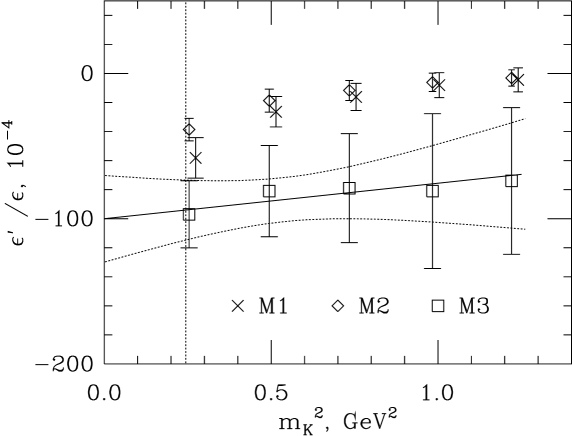
Figure 17: A rough estimate of $\varepsilon^{\prime}/\varepsilon$ for $Q_{1}$ ensemble using the partially-nonperturbative procedure described in text. Three sets of points correspond to using experimental $\mbox{Re}A_{0}$ and $\mbox{Re}A_{2}$ in Eq. (15) (crosses), using our $\mbox{Re}A_{0}$ but experimental $\omega$ (diamonds), or using $\mbox{Re}A_{0}$ and $\mbox{Re}A_{2}$ obtained from our calculations (squares). All other details are the same as in Table 3. The shown error is a combination of the statistical error, a matching error coming from uncertainties in the determination of $Z_{P}$ and $Z_{S}$, and an uncertainty in non-diagonal mixing of subdominant operators.

6 Estimates of $\varepsilon^{\prime}/\varepsilon$

Within the procedure outlined in the previous section we have found that $\langle O_{6}\rangle$ has a different sign from the expected one. This translates into a negative or very slightly positive value of $\varepsilon^{\prime}/\varepsilon$ (Tables 3 and 4 and Fig. 17).

If the assumptions about the subdominant diagrams made in the previous section are valid, our results would contradict the present experimental results, which favor a positive value of $\varepsilon^{\prime}/\varepsilon$. They would also change the existing theoretical picture [12] due to the change of sign of $\langle O_{6}\rangle$.

Finite volume and quenching effects were found small compared to noise. The main uncertainty in $\varepsilon^{\prime}/\varepsilon$ comes from operator matching, diagonal and non-diagonal. For diagonal matching the uncertainty comes from (1) errors in the determination of $Z_{P}$ and $Z_{S}$ non-perturbatively and from (2) unknown degree of validity of our ansatz in Sec. 5.3. For non-diagonal matching, the error is due to (3) unknown non-diagonal coefficients in mixing matrix and (4) ambiguity of accounting higher-order corrections. The error (1), as well as the statistical error, is quoted in Tables 3 and 4. The size of the error (4) can be judged by the spread in $\varepsilon^{\prime}/\varepsilon$ between two different approaches to higher-order corrections (strictly one-loop and partial resummation), also presented in Tables 3 and 4. The error (3) is likely to be of the same order as the error (4). The error (2) is uncontrolled at this point, since it is difficult to rigorously check our assumption made in Sec. 5.3. In Fig. 17 we combine the statistical error with errors (1) and (4) in quadrature.

The uncertainty due to operator matching is common to any method to compute the relevant matrix elements on the lattice (at least, with staggered fermions). In addition, our method has an inherent uncertainty due to dropping the higher order chiral terms. Lattice spacing dependence of $\varepsilon^{\prime}/\varepsilon$ is unclear at this point, but it may be significant.

We note that there are several ways to compute $\varepsilon^{\prime}/\varepsilon$. One can use the experimental values of $\mbox{Re}A_{0}$ and $\mbox{Re}A_{2}$ in Eq. (15), or one can use the values obtained on the lattice. One can also adopt an intermediate strategy of using the experimental amplitude ratio $\omega$ and computed $\mbox{Re}A_{0}$. When the higher-order chiral corrections are taken into account and the continuum limit is taken (so that $\omega=22$), these three methods should converge. At this point any of them can be used, and we compare them in Tables 3 and 4.

In view of the issues raised above, $\varepsilon^{\prime}/\varepsilon$ is an extremely fragile quantity. The rough estimates in Tables 3 and 4 and Fig. 17 should be used with extreme caution.

7 Conclusion

We have presented in detail the setup of our calculation of hadronic matrix elements of all operator in the basis defined in Eqs. (2—11). We have obtained statistically significant data for all operators. Based on these data we make theoretical estimates of $\mbox{Re}A_{0}$ and $\mbox{Re}A_{2}$ amplitudes as well as $\varepsilon^{\prime}/\varepsilon$.

Simulation results show that the enhancement of the $\Delta I=1/2$ transition is roughly consistent with the experimental findings. However, the uncertainty due to higher order chiral terms is very large. If these terms are calculated in the future, a more definite prediction for physical amplitudes can be obtained using our present data for matrix elements. Simulations should be repeated at a few more values of $\beta$ in the future in order to take the continuum limit.

Calculation of $\varepsilon^{\prime}/\varepsilon$ is further complicated by the failure of perturbation theory in operator matching. We give our crude estimates, but in order to achieve real progress the full nonperturbative matching procedure should be performed.

We appreciate L. Venkataraman’s help in developing CRAY-T3E software. We thank the Ohio Supercomputing Center and National Energy Research Scientific Computing Center (NERSC) for the CRAY-T3E time. We thank Columbia University group for access to their dynamical configurations.

Explicit expressions for fermion contractions

.1 Quark operators

We work in the two flavor traces formalism when calculating contractions with four-fermion operators: for each contraction separately the operators are rendered in the form (if necessary, by Fierz transformation) of two bilinears with the flavor flow in the form of a product of two flavor traces. To be more precise, for “eight” contractions the operators are rendered in the form $(\overline{s}\Gamma u)(\overline{u}\Gamma d)$, while for the “eye” and “annihilation” contractions the appropriate form is $(\overline{s}\Gamma d)(\overline{q}\Gamma q)$. This is done in the continuum, before assigning the staggered fermion flavour.

The operator transcription in flavor space for staggered fermions is now standard [10], and we give it here for completeness. The Goldstone bosons have spin-flavor structure $\gamma_{5}\otimes\xi_{5}$. The flavor structure of the operators is defined by requiring non-vanishing of the flavor traces, and so it depends on the contraction type: the flavor structure is $\xi_{5}$ in “eights” and two-point functions, ${\displaystyle\mathbf{1}}$ in “eyes” and “subtractions”. In “annihilation” contractions the flavour structure is ${\displaystyle\mathbf{1}}$ for the bilinear in the quark loop trace and $\xi_{5}$ for the one involved in the external trace.

Either one or two color traces may be appropriate for a particular contraction with a given operator (see the next Appendix section for details). In one trace contractions (type “F” for “fierzed”) the color flow is exchanged between the bilinears, while in two trace contractions (type “U” for “unfierzed”) the color flow is contained within each bilinear so that the contraction is the product of two color traces. In either contraction type, when the distance between staggered fermion fields being color-connected is non-zero, a gauge connector is inserted in the gauge-invariant fashion. The connector is computed as the average of products of gauge links along all shortest paths connecting the two sites. We also implement tadpole improvement by dividing each link in every gauge connector by $u_{0}=(1/3\mathrm{Tr}(U_{P}))^{1/4}$, where $U_{P}$ is the average plaquette value.

.2 Sources and contractions

We use local $U(1)$ pseudofermion wall sources. Explicitly, we set up a field of $U(1)$ phases $\xi_{\alpha}({\mathbf{x}};t_{0})$ ($|\xi_{\alpha}|=1$) for each color and each site at a given timeslice $t_{0}$, which are chosen at random and satisfy

$$\langle\xi_{\alpha}^{*}({\mathbf{x}};t_{0})\;\xi_{\beta}({\mathbf{y}};t_{0})\rangle=\delta_{\alpha,\beta}\;\delta_{{\mathbf{x}},{\mathbf{y}}}.$$ (38)

(Boldface characters designate spatial parts of the 4-vector with the same name.) We proceed to explain how this setup works in the case of the two-point function calculation, with trivial generalization to “eight” and “annihilation” contractions.

Consider the propagator from a wall at $t_{0}=0$ in a given background gauge configuration, computed by inverting the equation

$$(\hbox to0.0pt{\,/\hss}D+m)^{\alpha\beta}_{x\;y}\;\chi_{\beta}(y)=\xi_{\alpha}({\mathbf{x}};0)\delta_{x_{4},0}.$$ (39)

This is equivalent to computing

$$\chi_{\beta}(y)=\sum_{\mathbf{x}}\,\xi_{\alpha}({\mathbf{x}};0)G_{\beta\alpha}(y;{\mathbf{x}},0)\,,$$ (40)

where $G(y;x)$ is the propagator from 4-point x to 4-point y. For staggered fermions description we label the fields by hypercube index $h$ and the hypercube corner indices $A_{\mu}\in\{0,1\}^{4}$ instead of $y$. The two-point function is constructed as follows:

$${\mathrm{T}P}\propto\sum_{h,A}\chi^{*}_{\alpha}(h,A)U_{\alpha\beta}(h,A,A+\Delta)\chi_{\beta}(h,A+\Delta)\;\phi(A)\;(-1)^{A},$$ (41)

where $\phi(A)$ and $\Delta_{\mu}$ are phases and distances appropriate for a given staggered fermion operator , $U(h,A,A+\Delta)$ is the appropriate gauge connector (see below), modulo 2 summation is implied for hypercube indices $A$, and $h$ runs over all hypercubes in a given timeslice $t$ where the operator is inserted. The factor $(-1)^{A}$ takes into account that for staggered fermions $G(x;y)=G^{\dagger}(y;x)(-1)^{x}(-1)^{y}$. Equation (41) corresponds to

$${\mathrm{T}P}\propto\sum_{\mathbf{x},y,z}G_{\alpha\beta}(z,y)\;\Gamma\;G_{\beta\gamma}(y,x)\;(-1)^{z}\;\xi^{*}_{\alpha}(z)\xi_{\gamma}(x)\,,$$ (42)

where $\Gamma$ is used for simplicity to show the appropriate operator structure. The summation over ${\mathbf{x}}$ and ${\mathbf{z}}$ over the entire spatial volume averages over the noise, so the last equation is equivalent to

$${\mathrm{T}P}\propto\sum_{\mathbf{x},y}{\mathrm{t}r}\;G(x,y)\,\Gamma\,G(y,x)\;(-1)^{x}.$$ (43)

Therefore, using the pseudofermion wall source is equivalent to summation of contractions obtained with independent local delta-function sources. Note that the factor $(-1)^{x}$ and zero distance in the staggered fermions language are equivalent to spin-flavor structure $\gamma_{5}\otimes\xi_{5}$. This means the source creates pseudoscalar mesons at rest, which includes Goldstone bosons. Strictly speaking, this source also creates mesons with spin-flavor structure $\gamma_{5}\gamma_{4}\otimes\xi_{5}\xi_{4}$, since it is defined only on one timeslice. However, as explained in the first footnote in Section 2.3 of Ref. [10], these states do not contribute.

We have used one copy of pseudofermion sources per configuration.

Analogously, we construct the pion sink at time $T$ by using another set of $U(1)$ random noise ($\langle\xi_{\alpha}^{*}({\mathbf{x}};T)\;\xi_{\beta}({\mathbf{y}};T)\rangle=\delta_{\alpha,\beta}\;\delta_{{\mathbf{x}},{\mathbf{y}}}$, $|\xi|=1$). The propagator $\Phi$ is computed as follows:

$$(\hbox to0.0pt{\,/\hss}D+m)^{\alpha\beta}_{x\;y}\;\Phi_{\beta}(y)=\xi_{\alpha}({\mathbf{x}};T)\delta_{x_{4},T}.$$ (44)

Suppose $\Delta_{1}$, $\Delta_{2}\in\{0,1\}^{4}$ and $\phi_{1}(A)$, $\phi_{2}(A)$ are distances and phases of the two staggered fermion bilinears making up a given four-fermion operator. The expression for the “eight” contraction (Fig. 1a) with two color traces (“U” type) is given by

$${\mathrm{E}_{U}}\propto\sum_{h,A,B} \chi^{*}_{\alpha}(h,A)U_{\alpha\beta}(h,A,A+\Delta_{1})\chi_{\beta}(h,A+\Delta_{1})\;\phi_{1}(A)\;(-1)^{A}$$ (45)

$$\times\Phi^{*}_{\rho}(h,B)U_{\rho\sigma}(h,B,B+\Delta_{2})\Phi_{\sigma}(h,B+\Delta_{2})\;\phi_{2}(B)\;(-1)^{B},$$

up to various normalization factors which cancel in the $B$ ratio. In this expression $A$, $B\in\{0,1\}^{4}$ run over 16 hypercube corners (modulo 2 summation is implied for these indices). The hypercube index $h$, as before, runs over the entire spatial volume of the timeslice $t$ of the operator insertion. The gauge connector $U(h,A,B)$ is the identity matrix when $A=B$, otherwise it is the average of products of gauge links in the given configuration along all shortest paths from $A$ to $B$ in a given hypercube $h$. The expression (45), as well as all other contractions, is computed for each background gauge configuration and is subject to averaging over the configurations. (Whenever several contractions are combined in a single quantity, such as a $B$ ratio, we use jackknife to estimate the statistical error).

The expression for one color trace (“F” type) contraction is similar:

$${\mathrm{E}_{F}}\propto\sum_{h,A,B} \chi^{*}_{\alpha}(h,A)U_{\alpha\beta}(h,A,B+\Delta_{2})\chi_{\sigma}(h,A+\Delta_{1})\;\phi_{1}(A)\;(-1)^{A}$$ (46)

$$\times\Phi^{*}_{\rho}(h,B)U_{\rho\sigma}(h,B,A+\Delta_{1})\Phi_{\beta}(h,B+\Delta_{2})\;\phi_{2}(B)\;(-1)^{B},$$

For “eye” and “subtraction” diagrams (Fig. 1b and 1d) the source setup is a little more involved, since the kaon and pion are directly connected by a propagator. In order to construct a wall source we need to compute the product

$$\psi(y)=\sum_{\mathbf{x}}G({\mathbf{y}},t;{\mathbf{x}},T)\cdot G({\mathbf{x}},T;{\mathbf{0}},0)(-1)^{x}.$$

In order to avoid computing propagators from every point $\mathbf{x}$ at the timeslice $T$, we first compute propagator $G({\mathbf{x}},T;{\mathbf{0}},0)$, cut out the timeslice $T$ and use it as the source for calculating the propagator to $({\mathbf{y}},t)$. This amounts to inverting equation

$$(\hbox to0.0pt{\,/\hss}D+m)_{x\;y}^{\alpha\beta}\;\psi_{\beta}(y)=\chi_{\alpha}(x)\;\delta_{(x_{4},T)}(-1)^{x}\,,$$ (47)

where $\chi_{\alpha}(x)$ is the propagator from the wall source at $t_{0}=0$ defined in Eq. (39). We use the following expression for evaluating the “subtraction” diagram:

$${\mathrm{S}}\propto\sum_{h,A}\chi^{*}_{\alpha}(h,A)U_{\alpha\beta}(h,A,A+\Delta)\psi_{\beta}(h,A+\Delta)\;\phi(A)\;(-1)^{A},$$ (48)

Again, averaging over the noise leaves only local connections in both sources, so in the continuum language we get:

$${\mathrm{S}}\propto\sum_{\mathbf{x},y,z}{\mathrm{t}r}\;G({\mathbf{x}},0;{\mathbf{z}},t)\;\Gamma\;G({\mathbf{z}},t;{\mathbf{y}},T)\;G({\mathbf{y}},T;{\mathbf{x}},0)\;(-1)^{x}(-1)^{y}\,.$$ (49)

(In fact, we are mostly interested in subtracting the operator $\overline{s}{\displaystyle\mathbf{1}}\otimes{\displaystyle\mathbf{1}}d$, so in Eq. (48) $\Delta=\{0,0,0,0\}$ and $\phi(A)=1$.)

In order to efficiently compute fermion loops for “eye” and “annihilation” diagrams (Fig. 1b and 1c), we use $U(1)$ noise copies $\zeta^{(i)}$, $i=1,\dots,N$, at every point in space-time. We compute $\eta^{(i)}$ by inverting $(\hbox to0.0pt{\,/\hss}D+m)\eta^{(i)}=\zeta^{(i)}$. It is easy to convince oneself that the propagator from $y$ to $x$ equals

$$G(x;y)=\langle\eta_{x}\zeta_{y}^{*}\rangle.$$ (50)

In practice we average over $N=10$ noise copies. This includes 2 or 4 copies of the lattice in time extension, so the real number of noise copies is 20 or 40, with another factor of 3 for color. The efficiency of this method is crucial for obtaining good statistical precision.

The expression for “U” and “F” type “eye” diagrams are as follows:

$${\mathrm{I}_{U}} \propto\displaystyle\sum_{h,A,B} \chi^{*}_{\alpha}(h,A)U_{\alpha\beta}(h,A,A+\Delta_{1})\psi_{\beta}(h,A+\Delta_{1})\;\phi_{1}(A)\;(-1)^{A}$$

$$\times \displaystyle\frac{1}{N}\sum_{i=1}^{N} \zeta^{(i)*}_{\rho}(h,B)U_{\rho\sigma}(h,B,B+\Delta_{2})\eta^{(i)}_{\sigma}(h,B+\Delta_{2})\;\phi_{2}(B)\;(-1)^{B},$$ (51)

$${\mathrm{I}_{F}} \propto\displaystyle\sum_{h,A,B} \chi^{*}_{\alpha}(h,A)U_{\alpha\sigma}(h,A,B+\Delta_{2})\psi_{\beta}(h,A+\Delta_{1})\;\phi_{1}(A)\;(-1)^{A}$$

$$\times \displaystyle\frac{1}{N}\sum_{i=1}^{N} \zeta^{(i)*}_{\rho}(h,B)U_{\rho\beta}(h,B,A+\Delta_{1})\eta^{(i)}_{\sigma}(h,B+\Delta_{2})\;\phi_{2}(B)\;(-1)^{B}.$$ (52)

The computation of “annihilation” diagrams (Fig. 1c) is similar to the two-point function, except the fermion loop is added and the derivative with respect to the quark mass difference $m_{d}-m_{s}$ is inserted in turn in every strange quark propagator. Derivatives of the propagators are given by inverting equations

$$(\hbox to0.0pt{\,/\hss}D+m)\chi^{\prime} = \chi,$$ (53)

$$(\hbox to0.0pt{\,/\hss}D+m)\eta^{{}^{\prime}(i)} = \eta^{(i)}.$$ (54)

We have, therefore, four kinds of “annihilation” contractions, which should be combined in an appropriate way for each operator depending on the quark flavor structure (this is spelled out in the next Appendix section):

$${\mathrm{A}_{1U}} \propto\displaystyle\sum_{h,A,B} \chi^{{}^{\prime}*}_{\alpha}(h,A)U_{\alpha\beta}(h,A,A+\Delta_{1})\chi_{\beta}(h,A+\Delta_{1})\;\phi_{1}(A)\;(-1)^{A}$$

$$\times \displaystyle\frac{1}{N}\sum_{i=1}^{N} \zeta^{(i)*}_{\rho}(h,B)U_{\rho\sigma}(h,B,B+\Delta_{2})\eta^{(i)}_{\sigma}(h,B+\Delta_{2})\;\phi_{2}(B)\;(-1)^{B},$$ (55)

$${\mathrm{A}_{1F}} \propto\displaystyle\sum_{h,A,B} \chi^{{}^{\prime}*}_{\alpha}(h,A)U_{\alpha\sigma}(h,A,B+\Delta_{2})\chi_{\beta}(h,A+\Delta_{1})\;\phi_{1}(A)\;(-1)^{A}\nolinebreak$$

$$\times \displaystyle\frac{1}{N}\sum_{i=1}^{N} \zeta^{(i)*}_{\rho}(h,B)U_{\rho\beta}(h,B,A+\Delta_{1})\eta^{(i)}_{\sigma}(h,B+\Delta_{2})\;\phi_{2}(B)\;(-1)^{B},$$ (56)

$${\mathrm{A}_{2U}} \propto\displaystyle\sum_{h,A,B} \chi^{*}_{\alpha}(h,A)U_{\alpha\beta}(h,A,A+\Delta_{1})\chi_{\beta}(h,A+\Delta_{1})\;\phi_{1}(A)\;(-1)^{A}$$

$$\times \displaystyle\frac{1}{N}\sum_{i=1}^{N} \zeta^{(i)*}_{\rho}(h,B)U_{\rho\sigma}(h,B,B+\Delta_{2})\eta^{{}^{\prime}(i)}_{\sigma}(h,B+\Delta_{2})\;\phi_{2}(B)\;(-1)^{B},$$ (57)

$${\mathrm{A}_{2F}} \propto\displaystyle\sum_{h,A,B} \chi^{*}_{\alpha}(h,A)U_{\alpha\sigma}(h,A,B+\Delta_{2})\chi_{\beta}(h,A+\Delta_{1})\;\phi_{1}(A)\;(-1)^{A}\nolinebreak$$

$$\times \displaystyle\frac{1}{N}\sum_{i=1}^{N} \zeta^{(i)*}_{\rho}(h,B)U_{\rho\beta}(h,B,A+\Delta_{1})\eta^{{}^{\prime}(i)}_{\sigma}(h,B+\Delta_{2})\;\phi_{2}(B)\;(-1)^{B}.$$ (58)

Explicit expressions for matrix elements in terms of fermion contractions.

Operators in Eqs. (2—11) can be decomposed into $I=0$ and $I=2$ parts, which contribute, correspondingly, to $\Delta I=1/2$ and $\Delta I=3/2$ transitions. Here we give the expressions for these parts for completeness, since $\mbox{Re}A_{0}$, $\mbox{Re}A_{2}$ and $\varepsilon^{\prime}/\varepsilon$ are directly expressible in terms of their matrix elements. The $I=0$ parts are given as follows:

$$O_{1}^{(0)} = \frac{2}{3}(\overline{s}\gamma_{\mu}(1-\gamma_{5})d)(\overline{u}\gamma^{\mu}(1-\gamma_{5})u)-\frac{1}{3}(\overline{s}\gamma_{\mu}(1-\gamma_{5})u)(\overline{u}\gamma^{\mu}(1-\gamma_{5})d)$$ (59)

$$+ \frac{1}{3}(\overline{s}\gamma_{\mu}(1-\gamma_{5})d)(\overline{d}\gamma^{\mu}(1-\gamma_{5})d)$$

$$O_{2}^{(0)} = \frac{2}{3}(\overline{s}\gamma_{\mu}(1-\gamma_{5})u)(\overline{u}\gamma^{\mu}(1-\gamma_{5})d)-\frac{1}{3}(\overline{s}\gamma_{\mu}(1-\gamma_{5})d)(\overline{u}\gamma^{\mu}(1-\gamma_{5})u)$$ (60)

$$+ \frac{1}{3}(\overline{s}\gamma_{\mu}(1-\gamma_{5})d)(\overline{d}\gamma^{\mu}(1-\gamma_{5})d)$$

$$O_{3}^{(0)} = (\overline{s}\gamma_{\mu}(1-\gamma_{5})d)\sum_{q=u,d,s}(\overline{q}\gamma^{\mu}(1-\gamma_{5})q)$$ (61)

$$O_{4}^{(0)} = (\overline{s}_{\alpha}\gamma_{\mu}(1-\gamma_{5})d_{\beta})\sum_{q=u,d,s}(\overline{q}_{\beta}\gamma^{\mu}(1-\gamma_{5})q_{\alpha})$$ (62)

$$O_{5}^{(0)} = (\overline{s}\gamma_{\mu}(1-\gamma_{5})d)\sum_{q=u,d,s}(\overline{q}\gamma^{\mu}(1+\gamma_{5})q)$$ (63)

$$O_{6}^{(0)} = (\overline{s}_{\alpha}\gamma_{\mu}(1-\gamma_{5})d_{\beta})\sum_{q=u,d,s}(\overline{q}_{\beta}\gamma^{\mu}(1+\gamma_{5})q_{\alpha})$$ (64)

$$O_{7}^{(0)} = \frac{1}{2}[(\overline{s}\gamma_{\mu}(1-\gamma_{5})d)(\overline{u}\gamma^{\mu}(1+\gamma_{5})u)-(\overline{s}\gamma_{\mu}(1-\gamma_{5})u)(\overline{u}\gamma^{\mu}(1+\gamma_{5})d)$$ (65)

$$- (\overline{s}\gamma_{\mu}(1-\gamma_{5})d)(\overline{s}\gamma^{\mu}(1+\gamma_{5})s)]$$

$$O_{8}^{(0)} = \frac{1}{2}[(\overline{s}_{\alpha}\gamma_{\mu}(1-\gamma_{5})d_{\beta})(\overline{u}_{\beta}\gamma^{\mu}(1+\gamma_{5})u_{\alpha})-(\overline{s}_{\alpha}\gamma_{\mu}(1-\gamma_{5})u_{\beta})(\overline{u}_{\beta}\gamma^{\mu}(1+\gamma_{5})d_{\alpha})$$ (66)

$$- (\overline{s}_{\alpha}\gamma_{\mu}(1-\gamma_{5})d_{\beta})(\overline{s}_{\beta}\gamma^{\mu}(1+\gamma_{5})s_{\alpha})]$$

$$O_{9}^{(0)} = \frac{1}{2}[(\overline{s}\gamma_{\mu}(1-\gamma_{5})d)(\overline{u}\gamma^{\mu}(1-\gamma_{5})u)-(\overline{s}\gamma_{\mu}(1-\gamma_{5})u)(\overline{u}\gamma^{\mu}(1-\gamma_{5})d)$$ (67)

$$- (\overline{s}\gamma_{\mu}(1-\gamma_{5})d)(\overline{s}\gamma^{\mu}(1-\gamma_{5})s)]$$

$$O_{10}^{(0)} = \frac{1}{2}[(\overline{s}\gamma_{\mu}(1-\gamma_{5})u)(\overline{u}\gamma^{\mu}(1-\gamma_{5})d)-(\overline{s}\gamma_{\mu}(1-\gamma_{5})d)(\overline{u}\gamma^{\mu}(1-\gamma_{5})u)$$ (68)

$$- (\overline{s}\gamma_{\mu}(1-\gamma_{5})d)(\overline{s}\gamma^{\mu}(1-\gamma_{5})s)]$$

Expressions for $I=2$ parts are as follows:

$$O_{1}^{(2)} = O_{2}^{(2)}=\frac{2}{3}O_{9}^{(2)}=\frac{2}{3}O_{10}^{(2)}=\frac{1}{3}[(\overline{s}\gamma_{\mu}(1-\gamma_{5})u)(\overline{u}\gamma^{\mu}(1-\gamma_{5})d)$$ (69)

$$+(\overline{s}\gamma_{\mu}(1-\gamma_{5})d)(\overline{u}\gamma^{\mu}(1-\gamma_{5})u)-(\overline{s}\gamma_{\mu}(1-\gamma_{5})d)(\overline{d}\gamma^{\mu}(1-\gamma_{5})d)]$$

$$O_{7}^{(2)} = \frac{1}{2}[(\overline{s}\gamma_{\mu}(1-\gamma_{5})u)(\overline{u}\gamma^{\mu}(1+\gamma_{5})d)$$ (70)

$$+(\overline{s}\gamma_{\mu}(1-\gamma_{5})d)(\overline{u}\gamma^{\mu}(1+\gamma_{5})u)-(\overline{s}\gamma_{\mu}(1-\gamma_{5})d)(\overline{d}\gamma^{\mu}(1+\gamma_{5})d)]$$

$$O_{8}^{(2)} = \frac{1}{2}[(\overline{s}_{\alpha}\gamma_{\mu}(1-\gamma_{5})u_{\beta})(\overline{u}_{\beta}\gamma^{\mu}(1+\gamma_{5})d_{\alpha})$$ (71)

$$+(\overline{s}_{\alpha}\gamma_{\mu}(1-\gamma_{5})d_{\beta})(\overline{u}_{\beta}\gamma^{\mu}(1+\gamma_{5})u_{\alpha})-(\overline{s}_{\alpha}\gamma_{\mu}(1-\gamma_{5})d_{\beta})(\overline{d}_{\beta}\gamma^{\mu}(1+\gamma_{5})d_{\alpha})]$$

$$O_{3}^{(2)} = O_{4}^{(2)}=O_{5}^{(2)}=O_{6}^{(2)}=0$$ (72)

(Whenever the color indices are not shown, they are contracted within each bilinear, i.e. there are two color traces.)

As mentioned in Sec. 3.2, in order to compute matrix elements of $I=0$ operators one needs to evaluate three types of diagrams: “eight” (Fig. 1a), “eye” (Fig. 1b) and “annihilation” (Fig. 1c). In the previous Appendix section we have given detailed expressions for computation of these contractions, given the spin-flavor structure. Here we assign this structure to all contractions required for each operator, i.e. we express each matrix element in terms of contractions which were “built” in the previous section.

Let us introduce some notation. Matrix element of the above operators have three components:

$$\langle\pi^{+}\pi^{-}|O_{i}|K^{0}\rangle=(E_{i}+I_{i}-S\,(\,2\,m\alpha_{i})\,)\,\frac{m_{K}^{2}-m_{\pi}^{2}}{(p_{\pi}\cdot p_{K})f},$$ (73)

where $m$ is the common quark mass for $s$, $d$ and $u$, and

$$\alpha_{i}=\frac{A_{i}}{P}.$$ (74)

Here $E_{i}$ and $I_{i}$ stand for “eight and “eye” contractions of the $\langle\pi^{+}|O_{i}|K^{+}\rangle$ matrix element, $A_{i}\sim\langle 0|O_{i}|K^{0}\rangle\,/\,(m_{d}-m_{s})$ is the “annihilation” diagram, $S=\langle\pi^{+}|\overline{s}d|K^{+}\rangle$ is the “subtraction” diagram, and $P=\langle 0|\overline{s}\gamma_{5}d|K^{0}\rangle$ is the two-point function. We compute $\alpha_{i}$ by averaging the ratio in the right-hand side of Eq. (74) over a suitable time range.

Detailed expressions for $E_{i}$, $I_{i}$ and $A_{i}$ are given below in terms of the basic contractions on the lattice. We label basic contractions by two letters, each representing a bilinear. For example, $PP$ stands for contraction of the operator with spin structure $(\gamma_{5})(\gamma_{5})$, $SS$ is for $({\displaystyle\mathbf{1}})({\displaystyle\mathbf{1}})$, $VV$ stands for $(\gamma_{\mu})(\gamma^{\mu})$, and $AA$ is for $(\gamma_{\mu}\gamma_{5})(\gamma^{\mu}\gamma_{5})$. The staggered flavor is determined by the type of contraction, as explained in the previous Appendix section. Basic contractions are also labeled by their subscript. The first letter indicates whether it is an “eight”, “eye” or “annihilation” contraction, and the second is “U” for two, or “F” for one color trace. For example: $PP_{EU}$ stands for the “eight” contraction of the operator with spin-flavor structure $(\gamma_{5}\otimes\xi_{5})(\gamma_{5}\otimes\xi_{5})$ with two color traces; $VA_{A1F}$ stands for the “annihilation” contraction of the first type, in which the derivative is taken with respect to quark mass on the external leg (see the previous Appendix section), the spin-flavor structure is $(\gamma_{\mu}\otimes\xi_{5})(\gamma^{\mu}\gamma_{5}\otimes{\displaystyle\mathbf{1}})$, and one color trace is taken. What follows are the full expressions.

“Eight” parts:

$$E_{1}^{(0)} = \frac{2}{3}(VV_{EF}+AA_{EF})-\frac{1}{3}(VV_{EU}+AA_{EU})$$ (75)

$$E_{2}^{(0)} = \frac{2}{3}(VV_{EU}+AA_{EU})-\frac{1}{3}(VV_{EF}+AA_{EF})$$ (76)

$$E_{3}^{(0)} = VV_{EF}+AA_{EF}$$ (77)

$$E_{4}^{(0)} = VV_{EU}+AA_{EU}$$ (78)

$$E_{5}^{(0)} = 2(PP_{EF}-SS_{EF})$$ (79)

$$E_{6}^{(0)} = 2(PP_{EU}-SS_{EU})$$ (80)

$$E_{7}^{(0)} = SS_{EF}-PP_{EF}+\frac{1}{2}(VV_{EU}-AA_{EU})$$ (81)

$$E_{8}^{(0)} = SS_{EU}-PP_{EU}+\frac{1}{2}(VV_{EF}-AA_{EF})$$ (82)

$$E_{9}^{(0)} = -E_{10}^{(0)}=\frac{1}{2}(VV_{EF}+AA_{EF}-VV_{EU}-AA_{EU})$$ (83)

$$E_{1}^{(2)} = E_{2}^{(2)}=\frac{2}{3}E_{9}^{(2)}=\frac{2}{3}E_{10}^{(2)}=\frac{1}{3}(VV_{EU}+AA_{EU}+VV_{EF}+AA_{EF})$$ (84)

$$E_{3}^{(2)} = E_{4}^{(2)}=E_{5}^{(2)}=E_{6}^{(2)}=0$$ (85)

$$E_{7}^{(2)} = \frac{1}{2}(AA_{EU}-VV_{EU})+SS_{EF}-PP_{EF}$$ (86)

$$E_{8}^{(2)} = \frac{1}{2}(AA_{EF}-VV_{EF})+SS_{EU}-PP_{EU}$$ (87)

“Eye” parts:

$$I_{1}^{(0)} = VV_{IU}+AA_{IU}$$ (88)

$$I_{2}^{(0)} = VV_{IF}+AA_{IF}$$ (89)

$$I_{3}^{(0)} = 3(VV_{IU}+AA_{IU})+2(VV_{IF}+AA_{IF})$$ (90)

$$I_{4}^{(0)} = 3(VV_{IF}+AA_{IF})+2(VV_{IU}+AA_{IU})$$ (91)

$$I_{5}^{(0)} = 3(VV_{IU}-AA_{IU})+4(PP_{IF}-SS_{IF})$$ (92)

$$I_{6}^{(0)} = 3(VV_{IF}-AA_{IF})+4(PP_{IU}-SS_{IU})$$ (93)

$$I_{7}^{(0)} = 2(PP_{IF}-SS_{IF})$$ (94)

$$I_{8}^{(0)} = 2(PP_{IU}-SS_{IU})$$ (95)

$$I_{9}^{(0)} = VV_{IF}+AA_{IF}$$ (96)

$$I_{10}^{(0)} = VV_{IU}+AA_{IU}$$ (97)

“Annihilation” parts are obtained by inserting the derivative with respect to $(m_{d}-m_{s})$ into every propagator involving the strange quark:

$$A_{1}^{(0)} = -(VA_{A1U}+AV_{A1U})$$ (98)

$$A_{2}^{(0)} = -(VA_{A1F}+AV_{A1F})$$ (99)

$$A_{3}^{(0)} = -3(VA_{A1U}+AV_{A1U})-(VA_{A2U}+AV_{A2U})$$ (100)

$$-2(VA_{A1F}+AV_{A1F})-(VA_{A2F}+AV_{A2F})$$

$$A_{4}^{(0)} = -3(VA_{A1F}+AV_{A1F})-(VA_{A2F}+AV_{A2F})$$ (101)

$$-2(VA_{A1U}+AV_{A1U})-(VA_{A2U}+AV_{A2U})$$

$$A_{5}^{(0)} = 3(VA_{A1U}-AV_{A1U})+(VA_{A2U}-AV_{A2U})+2(PS_{A2F}-SP_{A2F})$$ (102)

$$A_{6}^{(0)} = 3(VA_{A1F}-AV_{A1F})+(VA_{A2F}-AV_{A2F})+2(PS_{A2U}-SP_{A2U})$$ (103)

$$A_{7}^{(0)} = \frac{1}{2}(VA_{A2U}-AV_{A2U})+(PS_{A2F}-SP_{A2F})$$ (104)

$$A_{8}^{(0)} = \frac{1}{2}(VA_{A2F}-AV_{A2F})+(PS_{A2U}-SP_{A2U})$$ (105)

$$A_{9}^{(0)} = VA_{A1F}+AV_{A1F}+\frac{1}{2}(VA_{A2U}+AV_{A2U}+VA_{A2F}+AV_{A2F})$$ (106)

$$A_{10}^{(0)} = VA_{A1U}+AV_{A1U}+\frac{1}{2}(VA_{A2F}+AV_{A2F}+VA_{A2U}+AV_{A2U})$$ (107)

Of course, “eye” and “annihilation” contractions are not present in $I=2$ operators.

TABLES

Table 3: $\varepsilon^{\prime}/\varepsilon$ in units of $10^{-4}$ for $Q_{1}$ ensemble, computed in three ways: (M1) $\mbox{Re}A_{0}$ and $\mbox{Re}A_{2}$ values entering the expression for $\varepsilon^{\prime}/\varepsilon$ are taken from experiment; (M2) $\omega$ amplitude ratio is taken from experiment, while $\mbox{Re}A_{0}$ amplitude is from our simulation; (M3) both $\mbox{Re}A_{0}$ and $\mbox{Re}A_{2}$ are from our simulation. Partially-nonperturbative matching have been used to obtain the results. In all perturbative corrections we have used one-loop coefficients computed for gauge-noninvariant operators. The first error is statistical (obtained by combining the individual errors in matrix elements by jackknife). The second error is the diagonal operator matching error due to uncertainty in the determination of $Z_{P}$ and $Z_{S}$. In order to estimate the non-diagonal matching error we compare two renormalization procedures: using strictly one-loop non-diagonal corrections (denoted “(1l.)”), and resumming part of higher-order corrections in non-diagonal mixing by using non-perturbative renormalization factors $Z_{P}$ and $Z_{S}$ (as explained in Section 5.3). The latter method is denoted “(p.r.)”. Some other parameters used in obtaining these results are: $\mbox{Im}\lambda_{t}=1.5\cdot 10^{-4}$, $m_{t}=170$ GeV, $m_{b}=4.5$ GeV, $m_{c}=1.3$ GeV, $\Omega_{\eta+\eta^{\prime}}=0.25$, $\alpha^{(n_{f}=0)}_{\overline{\mathrm{M}S}}(2\quad{\mathrm{G}eV})=0.195$ (the latter is based on setting the lattice scale by $\rho$ meson mass). Short distance coefficients were obtained by two-loop running using the anomalous dimension and threshold matrices computed by Buras et al. [12].

Quark mass	0.01	0.02	0.03
M1 (p.r.)	$-58.1\pm 2.1\pm 10.6$	$-26.3\pm 0.8\pm 8.9$	$-16.1\pm 0.4\pm 8.0$
M1 (1l.)	$-52.3\pm 2.2\pm 10$	$-22.0\pm 0.8\pm 8.3$	$-12.2\pm 0.5\pm 6.9$
M2 (p.r.)	$-38.6\pm 2.1\pm 6.0$	$-18.7\pm 0.3\pm 7.0$	$-11.7\pm 0.2\pm 6.0$
M2 (1l.)	$-45.4\pm 3.5\pm 8.6$	$-18.8\pm 0.4\pm 7.0$	$-10.3\pm 0.3\pm 6.0$
M3 (p.r.)	$-97\pm 14\pm 13$	$-81\pm 4\pm 23$	$-79\pm 2\pm 27$
M3 (1l.)	$-142\pm 28\pm 29$	$-88\pm 5\pm 35$	$-75\pm 2\pm 39$
Quark mass	0.04	0.05
M1 (p.r.)	$-8.0\pm 0.9\pm 7.2$	$-4.4\pm 0.9\pm 7.2$
M1 (1l.)	$-4.2\pm 1.1\pm 6.5$	$-1.2\pm 1.0\pm 6.6$
M2 (p.r.)	$-6.1\pm 0.5\pm 5.3$	$-3.1\pm 0.5\pm 4.9$
M2 (1l.)	$-3.7\pm 0.8\pm 5.8$	$-0.9\pm 0.8\pm 5.2$
M3 (p.r.)	$-81\pm 5\pm 38$	$-74\pm 4\pm 38$
M3 (1l.)	$-64\pm 4\pm 52$	$-55\pm 5\pm 51$

Table 4: $\varepsilon^{\prime}/\varepsilon$ results for $Q_{3}$ ensemble ($\beta=6.2$). Everything else is the same as in Table 3.

Quark mass	0.010	0.015
M1 (p.r.)	$-109\pm 15\pm 84$	$-64\pm 7\pm 63$
M1 (1l.)	$-95\pm 16\pm 74$	$-52\pm 8\pm 56$
M2 (p.r.)	$-39\pm 9\pm 22$	$-22\pm 2\pm 18$
M2 (1l.)	$-48\pm 18\pm 33$	$-23\pm 3\pm 23$
M3 (p.r.)	$-30.0\pm 17\pm 23.2$	$-21.1\pm 2.3\pm 20.7$
M3 (1l.)	$-48\pm 42\pm 39$	$-24\pm 7\pm 28$
Quark mass	0.020	0.030
M1 (p.r.)	$-36\pm 4\pm 60$	$-19\pm 2\pm 38$
M1 (1l.)	$-27\pm 5\pm 54$	$-14\pm 2\pm 34$
M2 (p.r.)	$-13.7\pm 0.6\pm 20$	$-9.5\pm 0.6\pm 17$
M2 (1l.)	$-12.4\pm 1.1\pm 23.3$	$-8.1\pm 0.9\pm 18.5$
M3 (p.r.)	$-15.9\pm 1.8\pm 26.5$	$-10.8\pm 1.1\pm 21.6$
M3 (1l.)	$-14.7\pm 1.4\pm 31.1$	$-9.6\pm 0.8\pm 18.4$

References

- [1] G. D. Barr et al. (NA31 CERN), Phys. Lett. B 317 (1993) 233.
- [2] Gibbons et al. (E731 Fermilab), Phys. Rev. Lett 70 1203-1206, 1993.
- [3] G. Kilcup, Nucl. Phys. B (Proc. Suppl.) 20 (1991) 417 (LATTICE ’90); S. Sharpe, R. Gupta, G. Guralnik, G. Kilcup, A. Patel, Phys. Lett. 192B (1987) 149.
- [4] C. Bernard, T. Draper, G. Hockney, A. Soni, Nucl. Phys. B (Proc. Suppl.) 4 (1988) 483 (LATTICE ’87); C. Bernard, A. El-Khadra, A. Soni, Nucl. Phys. Proc. Suppl. 7A (1989) 277;
- [5] C. Bernard, A. Soni, Fermilab LATTICE (1988) 0155; Nucl. Phys. B (Proc. Suppl.) 17 (1990) 495 (LATTICE ’89).
- [6] M.B. Gavela, L. Maiani, S. Petrarca, G. Martinelli, O. Pene, C.T. Sachrajda, Nucl. Phys. (Proc. Suppl. 7A) (1989) 228; E. Franco, L. Maiani, G .Martinelli, A. Morelli, Nucl. Phys. B 317 (1989) 63; M.B. Gavela, L. Maiani, S. Petrarca, G. Martinelli, O. Pene, Phys. Lett. 211 B (1988) 139; Nucl. Phys. B (Proc. Suppl.) 4 (1988) 466.
- [7] S. Aoki et al. (JLQCD collaboration), Phys. Rev. D 58 (1998) 054503, hep-lat/9711046.
- [8] M. Ciuchini et al., Z. Phys. C 68 (1995) 239, hep-ph/9501265.
- [9] G. Kilcup, S. Sharpe, Nucl. Phys. B 283 (1987) 493.
- [10] S. Sharpe, A. Patel, R Gupta, G. Guralnik and G. Kilcup, Nucl. Phys. B 286 (1987) 253-292.
- [11] C. Bernard, T. Draper, A. Soni, H.D. Politzer and M. B. Wise, Phys. Rev. D 32 (1985) 2343.
- [12] A. Buras et al., Nucl. Phys. B 408 (1993) 209-285, hep-ph/9303284; A. Buras, hep-ph/9806471, to appear in “Probing the Standard Model of Particle Interactions”, F.David and R. Gupta, eds., 1998, Elsevier Science B.V.
- [13] A.Buras et al., Nucl. Phys. B 400 (1993) 37 (hep-ph/9211304); Buras et al., Nucl. Phys. B 400 (1993) 75 (hep-ph/9211321).
- [14] L. Maiani, M. Testa, Phys. Lett. B 245 (1990) 585.
- [15] F. R. Brown et al., Phys. Res. D 67 (1991) 1062.
- [16] D. Chen, R Mawhinney, Nucl. Phys. B (Proc. Suppl.) 53 (1997) 216 (Lattice ’96).
- [17] S. Gottlieb, Nucl. Phys. B (Proc Suppl.) 53 (1997) 155 ( LATTICE ’96).
- [18] M. Golterman, K.C. Leung, Phys. Rev. D 56 (1997) 2950, hep-lat/9702015.
- [19] R. Gupta, T. Bhattacharya, S. Sharpe, Phys. Rev. D 55 (1997) 4036.
- [20] J.F.Donoghue, E. Golowich, B.R.Holstein, Phys. Lett. B 119 (1982) 412.
- [21] G. Kilcup, D. Pekurovsky, Nucl. Phys. B (Proc. Suppl.) 53 (1997) 345 (LATTICE ’96), hep-lat/9609006.
- [22] JLQCD, Phys. Rev. Lett. 80 (1998) 5271.
- [23] D.Pekurovsky, G. Kilcup, in preparation.
- [24] S. Sharpe, A. Patel, hep-lat/9310004.
- [25] N. Ishizuka, Y. Shizawa, Phys. Rev. D 49 (1994) 3519, hep-lat/9308008.
- [26] S. Sharpe, Phys. Rev. D 46 (1992) 3146.
- [27] A. Donini, V. Gimenez, G. Martinelli, G.C. Rossi, M. Talevi, M. Testa, A. Vladikas, Nucl. Phys. B (Proc. Suppl.) 53 (1997) 883 (LATTICE ’96), hep-lat/9608108; A. Donini, G. Martinelli, C.T. Sachrajda, M. Talevi, A. Vladikas, Phys. Lett. B 360 (1995) 83, hep-lat/9508020.
- [28] G. Martinelli, C. Pittori, C.T. Sachrajda, M. Testa, A. Vladikas, Nucl. Phys. B 445 (1995) 81, hep-lat/9411010.