Coupling Constant and Quark Loop Expansion for Corrections to the Valence Approximation

Abstract

For full QCD vacuum expectation values we construct an expansion in quark loop count and in powers of a coupling constant. The leading term in this expansion is the valence (quenched) approximation vacuum expectation value. Higher terms give corrections to the valence approximation. A test of the expansion is presented for moderately heavy quarks on a small lattice. We consider briefly an application of the expansion to quarkonium-glueball mixing.

I INTRODUCTION

The infinite volume, continuum limit of lattice QCD hadron masses [2, 3, 4] and meson decay constants [5, 4] calculated in the valence (quenched) approximation lie not far from experiment. Calculations using the valence approximation, however, require significantly less computer time than those using full QCD. Thus, in at least some cases, the valence approximation can serve as a cheap, approximate substitute for full QCD. For this purpose it would be useful to have some way to determine quantitatively an estimate of the error arising from the valence approximation short of a direct comparison of the valence approximation with full QCD.

A possible method for finding the valence approximation’s error is given in Ref. [6]. In the present article, we describe an alternative form of the proposal in Ref. [6] which we believe will generally require less computer time. The expansion we describe can be applied to any choice of quark action but is given here only for Wilson quarks.

In full QCD, virtual quark-antiquark pairs produced by a chromoelectric field reduce the field’s intensity by a factor which depends both on the field’s momentum and on its intensity. In the valence approximation this factor, analogous to a dielectric constant, is approximated by its zero-field-momentum zero-field-intensity limit [7]. Our expression for the error in valence approximation vacuum expectation values consists of an expansion in quark-loop count and in powers of a coupling constant. The coupling constant expansion relies on ideas drawn from mean-field-improved perturbation theory [8]. Each term in the expansion requires as input the quantity $\Delta\beta$ given by $(6\eta^{2}/g^{2})-(6/g^{2})$, where $g$ is the gauge coupling constant of full QCD and $\eta$ is the dielectric constant entering the valence approximation. We determine $\Delta\beta$ analytically from mean-field-improved perturbation theory to second order in the coupling constant. A related calculation of $\Delta\beta$ without mean-field improvement is described in Ref. [9]. The remaining work of evaluating each term in the error expansion is done by a Monte Carlo algorithm.

The sum of all terms in the error expansion, in principle, gives the exact value of the valence approximation error for any choice of the $\Delta\beta$. In particular, the expansion remains correct independent of the accuracy of the second order perturbative expression for $\Delta\beta$. For a bad choice of $\Delta\beta$, however, valence approximation vacuum expectations will be far from their full QCD values and the error expansion will predict an error correspondly large.

We have tested our method so far only for vacuum polarization arising from quarks with about 1.8 times the strange quark mass and only for a collection of Wilson loop expectation values. For these cases, our method of estimating the valence approximation error is significantly faster than direct comparison between the valence approximation and full QCD. A test of the efficiency of our method for lighter quark masses and other vacuum expectation values we hope to return to elsewhere.

In addition to its use as an algorithm for finding valence approximation errors, the expansion we describe provides a systematic way to keep track of the quantities which need to be evaluated, by any method, to determine quark loop corrections to valence approximation vacuum expectation values. Toward the end of the present article, we present a brief, qualitative discussion of the valence approximation and corrections to the valence approximation for mixing between the lightest scalar glueball and scalar quarkonium states. We will show that a recent attempt [10] to determine glueball-quarkonium mixing misses two of the terms required for this calculation. As a consequence, we believe the calculation of Ref. [10] is not correct.

In Section II we introduce definitions. In Section III, we construct an expansion for the valence approximation error. In Section IV we discuss the weak coupling calculation of the shift between the coupling constant in full QCD and in the valence approximation. In Section V we describe a trial calculations using our expansion and error estimates. In Section VI we consider the valence approximation and its corrections for glueball-quarkonium mixing.

II DEFINITIONS

For euclidean QCD on some finite lattice, let $u(x,y)$ be a guage link with periodic boundary conditions, and let $M$ be the coupling matrix for a single quark flavor, with antiperiodic boundary conditions, defined by

$$M(x,y) = \delta_{xy}-\kappa\sum_{\mu}\delta_{xy-\hat{\mu}}(1-\gamma_{\mu})u(x,y)-\kappa\sum_{\mu}\delta_{xy+\hat{\mu}}(1+\gamma_{\mu})u(x,y).$$ (1)

The vector $\hat{\mu}$ is a unit lattice vector in the $+\mu$ direction and the $\gamma_{\mu}$ are $4\times 4$ hermitian euclidean gamma-matrices.

For $n_{f}$ degenerate flavors of quarks and any integrable function of the gauge fields $G$, the vacuum expectation value found after integrating out quark fields becomes

$$<G> = Z^{-1}\int d\nu\,G\,det(M)^{n_{f}}\,exp(\frac{\beta}{6}P),$$ (2)

$$Z = \int d\nu\,det(M)^{n_{f}}\,exp(\frac{\beta}{6}P),$$ (3)

$$P = \sum_{(x_{1},\ldots x_{4})}Tr[u(x_{1},x_{2})u(x_{2},x_{3})u(x_{3},x_{4})u(x_{4},x_{1})].$$ (4)

Here $\beta$ is $6/g^{2}$ for bare gauge coupling constant $g$, $\nu$ is the product of one copy of $SU(3)$ Haar measure for each link variable on the lattice, and the sum in the definition of $P$ is over all nearest neighbor squares $(x_{1},\ldots x_{4})$ with squares differing by a cyclic permutation identified. The extension of Eq. (2) to vacuum expectations of products of quark and antiquark fields and to QCD with quarks having several different masses is not needed for the present discussion and will be omitted for simplicity. In the present discussion, $n_{f}$ can be either even or odd.

The valence approximation for $<G>$ is

$$<G>_{v} = Z_{v}^{-1}\int d\nu\,G\,exp(\frac{{\beta}_{v}}{6}P),$$ (5)

$$Z_{v} = \int d\nu\,exp(\frac{{\beta}_{v}}{6}P).$$ (6)

Here $\beta_{v}$ is $6/{g_{v}}^{2}$ with valence approximation bare gauge coupling $g_{v}$. It is convenient to name the shift between ${\beta}_{v}$ and $\beta$

$$\Delta\beta = {\beta}_{v}-\beta.$$ (7)

The determination of $\Delta\beta$ will be discussed in Section IV. As mentioned in Section I, $g_{v}$ and $g$ may also be viewed as related by a dielectric constant $\eta$

$$g_{v} = \frac{g}{\eta}.$$ (8)

The calculation of $\Delta\beta$ in Section IV is, in effect, also a calculation of $\eta$. Although $\eta$ is useful in describing the intuitive content of the valence approximation, it will not appear directly in the remainder of this paper.

III ERROR EXPANSION

A coupling constant and quark loop expansion can now be constructed for the difference between the full QCD vacuum expectation $<G>$ and its valence approximation $<G>_{v}$.

It is convenient [6] to express $<G>$ of Eq. (2) as

$$<G> = Z^{-1}\int d\nu\,G\,exp(\frac{{\beta}_{v}}{6}P+Q)$$ (9)

$$Z = \int d\nu\,exp(\frac{{\beta}_{v}}{6}P+Q),$$ (10)

$$Q = n_{f}tr{\log}(M)-\frac{\Delta\beta}{6}P.$$ (11)

Introducing a parameter $\lambda$ multiplying $Q$, we expand $<G>$ in powers of $\lambda$, replace $\lambda$ by 1, and get

$$<G> = <G>_{v}+\sum_{n}\delta_{n}(G),$$ (12)

$$\delta_{1}(G) = <(G-<G>_{v})(Q-<Q>_{v})>_{v},$$ (13)

$$\delta_{2}(G) = <(G-<G>_{v})(Q-<Q>_{v})^{2}>_{v},$$ (14)

$$\delta_{3}(G) = <(G-<G>_{v})(Q-<Q>_{v})^{3}>_{v}-$$ (16)

$$3<(G-<G>_{v})(Q-<Q>_{v})>_{v}<(Q-<Q>_{v})^{2}>_{v},$$

$$\vdots$$ (17)

In a coupling constant perturbation expansion of Eq. 12 for the difference between $<G>$ and $<G>_{v}$, the quantity $Q$ carries a single quark loop. As a consequence $\delta_{n}(G)$ can be associated with diagrams containing $n$ internal quark loops. None of the $\delta_{n}(G)$, however, are simply sums of $n$-quark-loop diagrams . Each includes also, through $Q$, counterterms arising from the shift between $\beta$ of full QCD and the screened $\beta_{v}$ of the valence approximation. We will return to this observation in Section VI.

The quantity $tr{\log}(M)$ in $Q$ of Eq. 9 we now express as a coupling constant power series. This series is also, formally, an expansion in powers of a gauge potential. Thus, as usual in gauge field theories, we use the theory’s gauge invariance to transform to a gauge which will tend to make the gauge potential small. For this purpose, we transform the gauge field $u(x,y)$ to a euclidean lattice version of Landau gauge. The field $u(x,y)$ has been transformed to lattice Landau gauge if for every lattice site $x$ the target function $\sum_{y}tr[u(x,y)]$ is a local maximum with respect to further gauge transformations. Generally there are many Gribov copies of transformations taking a particular gauge field to euclidean lattice Landua gauge. The vacuum expectation value of any integrable function of the gauge field transformed to Landau gauge is then an weighted average over the Gribov copies of each field. The weights depend on the particular choice of algorithm for obtaining Landau gauge. The gauge fixing algorithm used in our trial calculation in Section III is discussed in Ref. [6]. Our expansion does not depend explicitly on the choice of gauge fixing algorithm and, therefore, on the choice of Gribov copy weighting. We have not examined to what degree this choice might be optimized to further minimize the gauge potential and therefore speed the convergence of the coupling constant expansion.

For each fixed gauge configuration, we construct a free quark coupling matrix $M_{0}$ which approximates the interacting coupling matrix $M$ of Eq. 1. For each configuration, let $z$ be the average over all lattice links of $tr[u(x,y)]/3$. Let $M_{0}$ be a free coupling matrix with hopping constant $\kappa_{0}$ chosen to give a quark mass with agrees with the mean-field-improved [8] estimate

$$\frac{1}{2\kappa_{0}}-4 = \frac{1}{2z\kappa}-\frac{1}{2z\kappa_{c}},$$ (18)

where $\kappa$ and $\kappa_{c}$ are, respectively, the hopping constant of $M$ and the valence approximation to the critical value of this hopping constant. The critical hopping constant is the smallest value for which the pion mass becomes zero. On the right side of Eq. 18, the parameter $z$ varies with gauge configuration but $\kappa$ and $\kappa_{c}$ do not.

Mean-field improved perturbation theory suggests $zM_{0}$ as an approximation to $M$. We therefore express $tr{\log}(M)$ in the form

$$tr{\log}(M)=tr{\log}\{zM_{0}[1-M_{0}^{-1}(M_{0}-z^{-1}M)]\},$$ (19)

and expand to obtain the

$$tr{\log}(M)=tr{\log}(zM_{0})-\sum_{n}\frac{1}{n}tr\{[M_{0}^{-1}(M_{0}-z^{-1}M)]^{n}\}.$$ (20)

For small values of the chromoelectric potential, $M_{0}^{-1}(M_{0}-z^{-1}M)$ is linear in the potential. Thus Eq. (20) is approximately an expansion in power of the chromoelectric potential or, equivalently, in powers of a coupling constant.

To evaluate the trace in the second term of Eq. (20) we use an ensemble of complex-valued quark fields $\phi$. For each site $x$ and each of the 12 combinations of spin index $s$ and color index $c$, the corresponding $\phi_{sc}(x)$ we take to be an independent complex random variable with absolute value 1 and probability distribution uniform on the unit circle. For an $R$ element ensemble of such fields $\phi^{r}$, $1\leq r\leq R$, we then have

$$tr{\log}(M)=tr{\log}(zM_{0})-R^{-1}\sum_{nr}\frac{1}{n}<\phi^{r},[M_{0}^{-1}(M_{0}-z^{-1}M)]^{n}\phi^{r}>.$$ (21)

Here $<\ldots,\ldots>$ is the inner product

$$<\phi,\phi^{\prime}> = \sum_{xsc}\phi^{*}_{sc}(x)\phi^{\prime}_{sc}(x)$$ (22)

on the space of complex-valued quark fields. In Eq. (21) the quantity $tr{\log}(zM_{0})$ and the inverse $M_{0}^{-1}$ can be both be found easily in momentum space since $M_{0}$, in momentum space, is block-diagonal. To multiply vectors specified in position space by $M_{0}^{-1}$, we transform in and out of momentum space by fast Fourier transforms.

If the right side of Eq. (21) is substituted for $tr{\log}(M)$ in the expression for $Q$ in Eq. 9, Eq. 12 becomes a coupling constant and quark-loop expansion for corrections to valence approximation vacuum expectation values. The only quantity in this expansion not yet specified is the shift $\Delta\beta$. Eqs. (12) and (21) are formally correct for any choice of $\Delta\beta$. The rate at which these series converge, however, will be affected by this choice.

IV $\Delta\beta$

For valence approximation calculations of the light hadron spectrum, the up and down quark masses are usually taken to be equal and the corresponding $\kappa$ is chosen by requiring the pion mass to have its physical value. The valence approximation $\beta_{v}$ is then determined by setting the rho mass to its physical value. Thus, in effect, $\Delta\beta$ is found by requiring the valence approximation error in the rho mass to vanish. Since the rho mass is expected to be determined mainly by the low-momentum behavior of the chromoelectric field, this choice may be viewed as a quantitative implementation of the qualitative picture of the valence approximation mentioned briefly in Sect. I. A class of possible alternatives consists of choices of $\Delta\beta$ which make the error, or some approximation to the error, equal to zero for other quantities beside the rho mass which are determined mainly by the low-momentum behavior of the chromoelectric field. A convenient version of this idea for the present discussion is to fix $\Delta\beta$ by requiring zero valence approximation error for the Landau gauge gluon propagator at minimal nonzero momentum to first order in quark loops and to second order in the coupling constant expansion. As an additional simplification, the expectation values needed to determine $\Delta\beta$ we find using (analytic) mean-field-improved perturbation theory rather than by Monte Carlo. For the test case considered in Section III, we obtain the same value of $\Delta\beta$ by this method as produced by the non-perturbative method of Ref. [6].

The requirement for $\Delta\beta$ becomes that $\delta_{1}(G)$ of Eq. 13 vanishes

$$<(G-<G>_{v})(Q-<Q>_{v})>_{v} = 0,$$ (23)

where

$$G = \sum_{c\mu}\tilde{A}_{c\mu}(p)\tilde{A}_{c\mu}(-p),$$ (24)

$$Q = -tr(V)-\frac{1}{2}tr(V^{2})-\frac{\Delta\beta}{6}P,$$ (25)

$$V = M_{0}^{-1}(M_{0}-z^{-1}M).$$ (26)

The quantity $\tilde{A}_{c\mu}(p)$ is the Fourier transformed gauge potential

$$\tilde{A}_{c\mu}(p) = \sum_{x}exp(-ip\cdot x)A_{c\mu}(x).$$ (27)

for momentum vector $p$ with a single nonzero component $p_{1}$ of $2\pi/L$, where $L$ is the lattice period, To second order in mean-field-improved perturbation theory, the link field $u(x,y)$, in $M$, and the plaquette action $P$ can be approximated by

$$u(x,x+\hat{\mu}) = z\{1-iA_{c\mu}(x+\frac{1}{2}\hat{\mu})T_{c}-\frac{1}{2}[A_{c\mu}(x+\frac{1}{2}\hat{\mu})T_{c}]^{2}\}$$ (28)

$$P = \frac{<trU>_{v}}{3}\sum_{xc\mu\nu}[1-\frac{1}{2}(F_{c\mu\nu}(x+\frac{1}{2}\hat{\mu}+\frac{1}{2}\hat{\nu})^{2}]$$ (29)

$$F_{c\mu\nu}(x) = A_{c\mu}(x+\frac{1}{2}\hat{\nu})-A_{c\mu}(x-\frac{1}{2}\hat{\nu})+A_{c\nu}(x-\frac{1}{2}\hat{\mu})-A_{c\nu}(x+\frac{1}{2}\hat{\mu}).$$ (30)

where the $T_{c}$ are an orthnormal basis for the Lie algebra of $SU(3)$

$$tr(T_{c}T_{d}) = \frac{1}{2}\delta_{cd},$$ (31)

and $<trU>_{v}$ is the valence approximation plaquette expectation value.

The vacuum expectation values in Eqs.32 we evaluate by lattice weak coupling perturbation theory to second order in the valence approximation coupling constant. This calculation reduces to finding the two vacuum polarization Feynman diagrams in Fig. 1. These diagrams for QCD are proportional to the corresponding diagrams for a $U(1)$ lattice gauge theory and thus fulfill the $U(1)$ theory’s Ward identities. The calculation of the tadpole diagram, Figure 1 (b) can thus be eliminated. We obtain

$$\Delta\beta = \frac{9n_{f}}{4\sin^{2}(\pi/L)<trU>_{v}}[\Pi_{22}(p)-\Pi_{22}(0)]$$ (32)

$$\Pi_{\mu\nu}(p) = \frac{1}{L^{4}}\sum_{q}tr[\Gamma_{\mu}(q+p/2)S(q+p)\Gamma_{\nu}(q+p/2)S(q)],$$ (33)

where each component of $q$ in the sum over $q$ ranges from $\pi/L$ to $2\pi-\pi/L$ in steps of $2\pi/L$. The propagator $S(q)$ and vertex $\Gamma_{\mu}(q)$ are

$$S(q) = \frac{1}{1/(2\kappa_{0})-i\sum_{\mu}\gamma_{\mu}sin(q_{\mu})-\sum_{\mu}cos(q_{\mu})},$$ (34)

$$\Gamma_{\mu}(q) = sin(q_{\mu})-i\gamma_{\mu}cos(q_{\mu}).$$ (35)

The limiting value of $\Delta\beta$ for large $L$ without mean-field improvement has been derived in Ref. [9].

V EXAMPLE

As a test of our method we compared valence approximation expectations $<G>_{v}$, Eq. (5), their one-loop errors $<(G-<G>_{v})(Q-<Q>_{v})>_{v}$, Eq. (12), and the corresponding full QCD expectations $<G>$, Eq. (9), for a lattice $10^{4}$ with $\beta_{v}$ of 5.679, $\kappa$ of 0.16 and $n_{f}$ of 2. For a $16^{3}\times 32$ lattice at $\beta_{v}$ of 5.70, Ref [2] gives a critical $\kappa_{c}$ of 0.16940(5) and strange quark mass $m_{s}a$ in lattice units of 0.097(3). Thus $\kappa$ of 0.16 corresponds to a quark mass about 1.8 times $m_{s}a$. According to Eq. (32), $\Delta\beta$ is 0.243 giving a full QCD $\beta$ of 5.436. For this case $\Delta\beta$ found by the method of Ref. [6] is 0.244(6).

We used 224 independent equilibrium gauge configuration in the valence approximation ensemble, generated by an over-relaxed pseudo heat bath algorithm, 600 random fermion fields $R$ to evaluate the trace in Eq. (21) and 176 weakly correlated equilibrium gauge configurations for the full QCD ensemble, generated by a red-black preconditioned hybrid Monte Carlo algorithm. The expansion in Eq. (21) was carried to order $n$ of 10. The calculation of $<(G-<G>_{v})(Q-<Q>_{v})>_{v}$ was not turned carefully. In particular $R$ of 600 in Eq. (21) is much larger than its optimal vaule. The time required for the valence approximation and error calculation was still less than 5% of the time required by the full QCD calculations.

For $G$ we used Wilson loops $W_{0},\ldots W_{10}$ consisting, respectively, of paths $1\times 1$, $2\times 1$, all rotations of steps in the directions $\hat{1},\hat{2},\hat{3},-\hat{1},-\hat{2},-\hat{3}$, all rotations of steps in the directions $\hat{1},\hat{2},\hat{3},-\hat{2},-\hat{1},-\hat{3}$, $3\times 1$, $2\times 2$, $4\times 1$, $5\times 1$, $3\times 2$, $4\times 2$, and $3\times 3$. For the $3\times 3$ loop, $W_{10}$, Fig. 2 shows the predicted error $<(W_{10}-<W_{10}>_{v})(Q-<Q>_{v})>_{v}$ as a function of the highest power $n$ of coupling strength used in Eq. (21). The error converges adequately by $n$ of 7. For smaller Wilson loops, $W_{0},\ldots W_{9}$, the predicted error’s convergence as a function of $n$ is comparable to or faster than the convergence shown in Fig. 2. For $n$ of 7, Fig. 3 shows the relative shift of the valence approximation from full QCD $(<W_{i}>-<W_{i}>_{v})/<W_{i}>$ and the predicted value $<(W_{i}-<W_{i}>_{v})(Q-<Q>_{v})>_{v}/<W_{i}>$. To within statistical uncertainties, the predicted errors agree with the true errors.

The true errors in Fig. 3 were found from the shortest full QCD run sufficient to confirm equilibration of $<W_{0}>,\ldots<W_{10}>$. Nonetheless the statistical uncertainties in the predicted errors are much larger than those in the true errors. If we were to run the error prediction algorithm long enough to obtain statistical uncertainties comparable to the uncertainties found by a direct comparison of full QCD and the valence approximation, it is possible that the computer time required by the error algorithm would become comparable to that for full QCD. To find the uncertainty arising from use of the valence approximation, however, the statistical uncertainty in the error estimate does not need to be too much smaller than the error estimate’s central value. Used in this way, for the set of parameters of the test, our algorithm takes significantly less time than the shortest possible direct comparison of the valence approximation and full QCD.

VI GLUEBALL-QUARKONIUM MIXING

We now consider briefly the valence approximation to glueball-quarkonium mixing, corrections to the valence approximation to mixing which follow from Eq. (12) and a mixing calculation reported in Ref. ([10]). The lowest lying glueball, according to the valence approximation, is stable and is expected to be a scalar. Evidence that $f_{0}(1710)$ is composed mainly of this state is given in Refs. [11, 12, 13, 14]. With quark-antiquark annihilation initially ignored, the lightest scalar quarkonium states are also stable. Their valence approximation masses and evidence for their identification with observed states are discussed in Refs. [15, 12, 13, 14].

Mixing among the $s\overline{s}$ and $(u\overline{u}+d\overline{d})/\sqrt{2}$ scalars and the scalar glueball then occurs through quark-antiquark annihilation. In the valence approximation, the glueball-quarkonium mixing energy can be extracted [13, 14] from the vacuum expectation value

$$C_{v}(t) = <g(t)s(0)>_{v},$$ (36)

where $g(\vec{x},t)$ is the smeared zero-momentum scalar glueball operator of Ref. [16], with vacuum expectation subtracted, and $s(\vec{x},t)$ is the smeared zero-momentum scalar quarkonium operator of Ref. [15]. It is convenient to define also a full QCD $C(t)$ by Eq. (36) with $<\ldots>_{v}$ replaced by $<\ldots>$. A qualitative representation of $C_{v}(t)$ is provided by Figure 4 giving a typical Feynman diagram contributing to the lattice weak coupling expansion for $C_{v}(t)$.

Assuming, for simplicity, only vacuum polarization arising from $u$ and $d$ quarks taken to have degenerate mass, the one-quark-loop correction to $C_{v}(t)$ can be found from Eqs. (9-13). For the present discussion, we will not apply the expansion of Eq. (20). The one-quark-loop error in $C_{v}(t)$ becomes

$$C(t)-C_{v}(t) = T_{M}-\frac{\Delta\beta}{6}T_{P},$$ (37)

$$T_{M} = <[g(t)s(0)-<g(t)s(0)>_{v}][2tr{\log}(M)-<2tr{\log}(M)>_{v}]>_{v}$$ (38)

$$T_{P} = <[g(t)s(0)-<g(t)s(0)>_{v}][P-<P>_{v}]>_{v}.$$ (39)

Qualitative representations of $T_{M}$ and $T_{P}$ are given by typical Feynman diagrams contributing to their weak coupling expansions shown in Figure 5(a) and Figure 5(b), respectively. Among the processes contributing to $T_{M}$ in Figure 5(a) are glueball-quarkonium transitions through common pi-pi, kaon-antikaon, and eta-eta decay channels. The quantity $T_{P}$, on the other hand, is the counterterm, discussed in Section III, which arises from the shift $\Delta\beta$ between $\beta$ of full QCD and the screened $\beta_{v}$ of the valence approximation.

In Ref. [10] a model is proposed for mixing among the valence approximation to the lightest scalar glueball state and the valence approximations to the lightest scalar $s\overline{s}$ and $(u\overline{u}+d\overline{d})/\sqrt{2})$ states. Applied to glueball-quarkonium mixing energies, this model omits the leading valence approximation mixing amplitude coming from $C_{v}(t)$ and represented in Figure 4. The model includes instead only transitions through common pi-pi, kaon-antikaon and eta-eta decay channels. These transition do contribute to $T_{M}$. Thus the model might be viewed as a calculation of quark-loop corrections to the valence approximation to mixing if not as an evaluation of the full mixing process. The equation assumed to govern mixing between the valence approximation glueball and quarkonium states through intermediate decay channels, however, entirely ignores the counter-term $T_{P}$. No argument is offered in support of this omission. Ref. [10] simply assumes, without proof, a relation between full QCD and valence approximation propagators with no term corresponding to $T_{P}$.

With this counter-term dropped, Eq. (37) gives the error in $C_{v}(t)$ for a version of the valence approximation with $\Delta\beta$ forced to zero. Equivalently, it is easily checked that $T_{P}$ is the derivative of $C_{v}(t)$ with respect to $\beta_{v}$. Thus by dropping the $T_{P}$ term from Eq. (37) the one-quark-loop error estimate for $C_{v}(t)$ is altered by approximately the increment in $C_{v}(t)$ in going from $\beta_{v}-\Delta\beta$ to $\beta_{v}$ . For $\beta_{v}$ of 5.93, $\Delta\beta$ is known to be greater than 0.23. Thus a lower bound on the effect of setting $\Delta\beta$ to zero can be found by comparing valence results at $\beta_{v}$ of 5.70 with those at $\beta_{v}$ of 5.93. The data in Refs. [13, 14] then shows that the one-quark-loop error estimate for glueball-quarkonium energy is changed by an amount equal to the entire leading valence approximation to the mixing energy obtained from $C_{v}(t)$.

A cross check on the consequences for valence approximation errors of forcing $\Delta\beta$ to zero can be obtained by making this change in the error formula applied to low-lying hadron masses and meson decay constants. Using the data in Refs. [2, 5] for $\beta_{v}$ of 5.70 and 5.93, we find that with $\Delta\beta$ forced to zero masses and decay constants are off by as much as 45%, rather than by less than 10% or less than 20%, respectively, for an optimally chosen $\Delta\beta$.

Thus as a calculation of errors in the valence approximation to glueball-quarkonium mixing energies, Ref. [10] would be expected to predict significantly larger errors than actually occur with an optimal choice of $\Delta\beta$. As we mentioned earlier, however, also missing from the calculation of Ref. [10] is the leading valence approximation term which can be obtained from $C_{v}(t)$. It appears to us that Ref. [10] gives neither an adequate model of the full glueball-quarkonium mixing process nor of the corrections to the leading valence approximation to this process. We believe its results are simply incorrect.

In partial defense of Ref. [10], it might be argued that although $T_{P}$ is not explicitly present in the relation given between valence approximation propagators and those of full QCD, $T_{P}$ is nonetheless present implicitly. The coupling between valence approximation states and two-body decay channels is assumed to fall exponentially with $|\vec{k}|^{2}$, where $\vec{k}$ is the center-of-mass system 3-momentum carried by one of the decay products. Perhaps this exponential cutoff removes from the equation of Ref. [10] those contributions which $T_{P}$ subtracts from our equations. For this to hold would require a surprising coincidence since no mention is made in Ref. [10] of the need for a term like $T_{P}$ in the relation between full QCD and the valence approximation and no attempt is made to tune the cutoff to absorb this term. The cutoff is introduced simply as the authors’ expectation of the behavior of coupling between unstable scalars and their pseudoscalar decay products.

In addition, however, it is mentioned explicitly in Ref. [10], and supported by the tables giving proposed values of full QCD corrections to valence approximation masses, that the model of Ref. [10] predicts full QCD masses below valence approximation masses for those states which are stable in the valence approximation but unstable in full QCD. This is exactly the result to be expected for corrections to the valence approximation given by Eqs. (12) and (13) with $T_{P}$ removed. For the vacuum expectation of an arbitrary $G$, Eqs. (12) and (13) give

$$<G>-<G>_{v} = T^{G}_{M}-\frac{\Delta\beta}{6}T^{G}_{P},$$ (40)

$$T^{G}_{M} = <(G-<G>_{v})[2tr{\log}(M)-<2tr{\log}(M)>_{v}]>_{v}$$ (41)

$$T^{G}_{P} = <(G-<G>_{v})(P-<P>_{v})>_{v}.$$ (42)

The contribution to the error in $<G>_{v}$ from the term $T^{G}_{M}$ is the incremental effect of the color charge screening due to a single quark loop and therefore of a decrease, by some amount, in the QCD effective charge. As a consequence of QCD’s asymptotic freedom this term shifts quantities with mass units toward smaller values in full QCD than in the valence approximation. From our discussion earlier it follows that the term $T^{G}_{P}$ has the opposite effect. It shifts quantities with mass units toward larger values in full QCD than in the valence approximation. In fact, as might be expected from the discussion of Ref. [12], calculations of valence approximation decay constants [5, 4] and a recent calculation of masses [4] show that full QCD quantities for excited states are consistently larger those of the valence approximation. Therefore $T^{G}_{P}$ for propagators of excited states is consistently larger in magnitude than $T^{G}_{M}$, and the model of Ref. [10] predicts even the wrong sign for the relation between masses in full QCD and in the valence approximation. It appears to us this error is clear evidence that the model’s cutoff on decay momenta can not have absorbed the effect of the omission of $T^{G}_{P}$.

FIG. 1.: Feynman diagrams which contribute to $\Delta\beta$.

FIG. 2.: The predicted relative shift in Wilson loop $W_{10}$ from its valence approximation value as a function of the order $n$ in coupling constant compared to the true shift of full QCD.

FIG. 3.: The predicted relative shift in 11 Wilson loops from their valence approximation values in comparison to the true shift of full QCD.

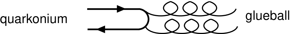
FIG. 4.: Quarkonium-glueball mixing through quark-antiquark annihilation.

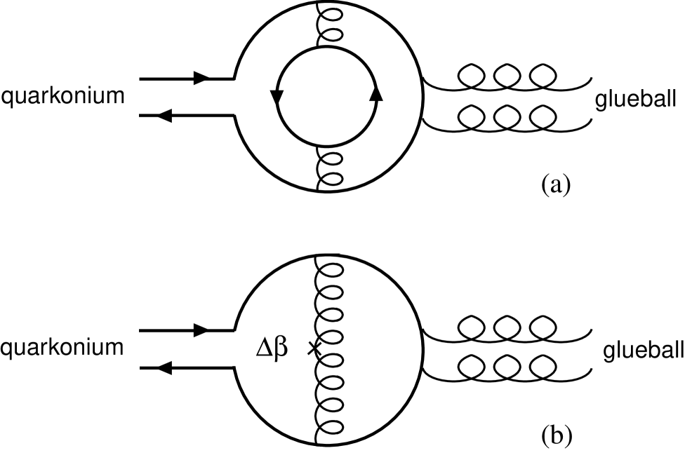
FIG. 5.: One-quark-loop corrections to the valence approximation to quarkonium-glueball mixing.

REFERENCES

- [1] Present address: Group T-8, Los Alamos National Laboratory, Los Alamos, NM 87545.
- [2] F. Butler, H. Chen, J. Sexton, A. Vaccarino and D. Weingarten, Phys. Rev. Lett. 70 (1993) 2849; Nucl. Phys. B430 (1994) 179.
- [3] C. Bernard, et al. Nucl. Phys. B (Proc. Suppl.) 47 (1996) 345; Nucl. Phys.] B (Proc. Suppl.) 53 (1997) 212.
- [4] S. Aoki, et al. Nucl. Phys. B (Proc. Suppl.) 63 (1998) 167.
- [5] F. Butler, H. Chen, J. Sexton, A. Vaccarino and D. Weingarten, Nucl. Phys. B 421 (1994) 217.
- [6] J. Sexton and D. Weingarten, Nucl. Phys. (Proc. Suppl.) 42 (1995) 361; Phys. Rev. D55 (1997) 4025.
- [7] D. H. Weingarten, Phys. Lett. 109B, 57 (1982); Nucl. Phys. B215 [FS7] (1983) 1.
- [8] G. P. Lepage and P. Mackenzie, Phys. Rev. D48 (1993) 2250.
- [9] A. Hasenfratz and T. DeGrand, Phys. Rev. D49, 466 (1994); Nucl. Phys. B (Proc. Suppl.) 34, 317 (1994).
- [10] M. Boglione and M. Pennington, Phys. Rev. Lett. 79, 1998 (1997).
- [11] J. Sexton, A. Vaccarino and D. Weingarten, Phys. Rev. Lett. 75, 4563 (1995).
- [12] D. Weingarten, Nucl. Phys. B (Proc. Suppl.) 53, 232 (1997).
- [13] W. Lee and D. Weingarten, Nucl. Phys. B (Proc. Suppl.) 63, 198 (1998).
- [14] W. Lee and D. Weingarten, IBM preprint IBMHET-98-1, hep-lat/9805029.
- [15] W. Lee and D. Weingarten, Nucl. Phys. B (Proc. Suppl.) 53, 236 (1997).
- [16] H. Chen, J. Sexton, A. Vaccarino and D. Weingarten, Nucl. Phys. B (Proc. Suppl.) 34, 357 (1994).