Small eigenvalues of the SU(3) Dirac operator
on the lattice and in Random Matrix Theory

Abstract

We have calculated complete spectra of the staggered Dirac operator on the lattice in quenched SU(3) gauge theory for $\beta=5.4$ and various lattice sizes. The microscopic spectral density, the distribution of the smallest eigenvalue, and the two-point spectral correlation function are analyzed. We find the expected agreement of the lattice data with universal predictions of the chiral unitary ensemble of random matrix theory up to a certain energy scale, the Thouless energy. The deviations from the universal predictions are determined using the disconnected scalar susceptibility. We find that the Thouless energy scales with the lattice size as expected from theoretical arguments making use of the Gell-Mann–Oakes–Renner relation.

The low-lying eigenvalues of the Dirac operator are of great importance for the understanding of spontaneous chiral symmetry breaking in an infinite volume [1]. On the lattice, however, one is always working at finite volume. Therefore, it is important to know how the thermodynamic limit is approached. It was shown by Leutwyler and Smilga [2] that in the domain

$$1/\Lambda\ll L\ll 1/m_{\pi}\>,$$ (1)

where $\Lambda$ is a typical hadronic scale, $L$ is the linear extent of the Euclidean box, and $m_{\pi}$ is the pion mass, the low-energy behavior of QCD can be described by a simple effective partition function whose existence imposes certain constraints on the eigenvalues of the Dirac operator. The spectrum of the Dirac operator in the domain (1) has been successfully predicted by chiral random matrix theory (RMT) [3, 4]. The only ingredients of the calculation are the global symmetries of the theory and the assumption that chiral symmetry is spontaneously broken. It has recently been shown that there is an overlap between the domain of validity of chiral RMT and of chiral perturbation theory, and that in this overlap region the two approaches yield the same results [5].

The results so obtained provide analytical information on the way in which the thermodynamic limit is approached. They are universal in the sense that they do not depend on the precise values of the parameters of the theory, i.e., of the simulation parameters on the lattice. However, the domain of validity of the universal results does depend on the parameters. The energy scale $\lambda_{\mathrm{RMT}}$ up to which RMT applies, i.e., the Thouless energy, follows from the upper bound on $L$ in relation (1) and the Gell-Mann–Oakes–Renner relation, $m_{\pi}^{2}f_{\pi}^{2}=2m\Sigma$, where $f_{\pi}=F_{\pi}/\sqrt{2}$ is the pion decay constant, $\Sigma$ is the absolute value of the chiral condensate $\langle\bar{\psi}\psi\rangle$, and $m$ is a valence quark mass. It is thus determined by [6, 7, 8]

$$\lambda_{\mathrm{RMT}}/\Delta\propto f_{\pi}^{2}L^{2}\>,$$ (2)

where $\Delta=1/\rho(0)=\pi/(V\Sigma)$ is the level spacing at zero. Here, $V=L^{4}$ denotes the four-volume, and $\rho(\lambda)=\langle\sum_{n}\delta(\lambda-\lambda_{n})\rangle_{A}$ is the spectral density of the Dirac operator averaged over gauge field configurations $A$. The relation between $\rho(0)$ and $\Sigma$ is given by the Banks–Casher formula, $\pi\rho(0)=V\Sigma$ [1].

The aim of this paper is (i) to test the universal predictions of chiral RMT for the distribution and correlations of the low-lying Dirac eigenvalues and (ii) to check the prediction of Eq. (2) for the Thouless energy, using lattice data computed in quenched SU(3) gauge theory with the staggered Dirac operator. Point (i) has previously been considered in quenched SU(2) [9, 10], in SU(2) with dynamical fermions [11], in quenched SU(3) in three dimensions [12], in U(1) in two dimensions [13], and, very recently, in quenched SU(3) in four dimensions [14]. Point (ii) has previously been tested in quenched SU(2) [15]. All these investigations were done with the staggered Dirac operator except for Ref. [13] in which the fixed point Dirac operator with respect to a renormalization group transformation was used. Since real QCD has three colors, SU(3) in four dimensions is clearly the most important case.

The Euclidean Dirac operator in the continuum is given by $i\hbox to0.0pt{\,/\hss}{{D}}=i\hbox to0.0pt{/\hss}{{\partial}}+gt^{a}\hbox to0.0pt{\,/\hss}{{A}}^{a}$, where the $t^{a}$ are the generators of the gauge group. The operator $i\hbox to0.0pt{\,/\hss}{{D}}$ is hermitean with real eigenvalues. It anticommutes with $\gamma_{5}$ and, therefore, all nonzero eigenvalues come in pairs $\pm\lambda_{n}$ with eigenvectors $\psi_{n},\gamma_{5}\psi_{n}$. There can also be zero modes which are either left-handed or right-handed. The topological charge of a given gauge field configuration is equal to the difference in the number of left-handed and right-handed zero modes. On the lattice, the staggered Dirac operator reads

$$(i\hbox to0.0pt{\,/\hss}{{D}})_{x,y}=\frac{i}{2}\sum_{\mu}\,\bigl{[} \eta_{\mu}(x)U_{\mu}(x)\cdot\delta_{x+\mu,y}$$ (4)

$$-\eta_{\mu}(y)U^{\dagger}_{\mu}(y)\cdot\delta_{x-\mu,y}\bigr{]}\>,$$

where $U$ and $\eta$ denote the link variables and the staggered phases, respectively.

The claim is that the distribution and the correlations of the small eigenvalues of $i\hbox to0.0pt{\,/\hss}{{D}}$ are described by universal functions which can be computed, e.g., in chiral RMT [3, 4]. The distribution of the low-lying eigenvalues is encoded in the spectral one-point function near zero virtuality, the so-called microscopic spectral density defined by [3]

$$\rho_{s}(z)=\lim_{V\to\infty}\frac{1}{V\Sigma}\,\rho\left(\frac{z}{V\Sigma}\right)\>.$$ (5)

Similarly, one considers the microscopic limit of the two-point cluster function,

$$\tau_{2}(z_{1},z_{2})=\lim_{V\to\infty}\frac{1}{(V\Sigma)^{2}}\,T_{2}\left(\frac{z_{1}}{V\Sigma},\frac{z_{2}}{V\Sigma}\right)$$ (6)

with

$$T_{2}(\lambda_{1},\lambda_{2})=\rho(\lambda_{1})\rho(\lambda_{2})-R_{2}(\lambda_{1},\lambda_{2})\>,$$ (7)

where $R_{2}(\lambda_{1},\lambda_{2})$ is the two-point spectral correlation function, i.e., the probability density that one eigenvalue is at $\lambda_{1}$ and another at $\lambda_{2}$, all other eigenvalues being unobserved.

For SU(3) with the staggered Dirac operator, the relevant symmetry class in the framework of chiral RMT is the chiral unitary ensemble [16]. In the following, we briefly summarize analytical results for this ensemble which are of relevance for the present work. The microscopic spectral density is given by [4]

$$\rho_{s}(z)=\frac{z}{2}\left[J_{\mu}^{2}(z)-J_{\mu+1}(z)J_{\mu-1}(z)\right]$$ (8)

with the Bessel function $J$ and $\mu=N_{f}+|\nu|$, where $N_{f}$ and $\nu$ denote the number of massless flavors and the topological charge, respectively. The distribution of the smallest eigenvalue for $N_{f}=\nu=0$ reads [17]

$$P(\lambda_{\min})=\frac{\lambda_{\min}}{2}\>e^{-\lambda_{\min}^{2}/4}\>.$$ (9)

The two-point cluster function in the microscopic limit is given by [4]

$$\tau_{2}(z_{1},z_{2})$$ (10)

$$= z_{1}z_{2}\left[\frac{z_{1}J_{\mu+1}(z_{1})J_{\mu}(z_{2})-z_{2}J_{\mu}(z_{1})J_{\mu+1}(z_{2})}{z_{1}^{2}-z_{2}^{2}}\right]^{2}\>.$$ (11)

The quantities in Eqs. (8) through (10) do not contain any free parameters. For a comparison with lattice data, the energy scale is determined by the parameter $V\Sigma$ which is obtained from the data by extracting $\rho(0)$ and applying the Banks–Casher relation, $\pi\rho(0)=V\Sigma$. Thus, the comparison between lattice data and the predictions of Eqs. (8) through (10) is parameter-free. (Strictly speaking, on finite lattices a spontanous breaking of chiral symmetry cannot occur and $\rho(0)$ is zero. The latter quantity must, therefore, be determined by extrapolating $\rho(\lambda)$ to $\lambda=0$. In practice, this extrapolation presents no difficulties.)

We now turn to the details of our numerical simulations. They were done in quenched SU(3) gauge theory with $\beta=6/g^{2}=5.4$ on lattices of size $V=L^{4}$ with $L=4$, 6, 8, 10. The boundary conditions are periodic for the gauge fields and periodic in space and anti-periodic in Euclidean time for the Dirac operator. The gauge field configurations were generated using a combined Metropolis and overrelaxation algorithm on the link variables. Two consecutive configurations are separated by at least 30 runs of one Metropolis sweep with three hits and 20 overrelaxation sweeps using Creutz’s method [18]. The complete spectrum of the staggered Dirac operator was then calculated using the Cullum–Willoughby version of the Lanczos algorithm for the matrix of $-\hbox to0.0pt{\,/\hss}{{D}}^{2}$. This operator couples only even to even and odd to odd lattice sites. Both blocks have the same eigenvalues. Hence it is sufficient to consider only even lattice sites. The eigenvalues of $-\hbox to0.0pt{\,/\hss}{{D}}^{2}$ were checked against the identity ${\mathrm{Tr}}(-\hbox to0.0pt{\,/\hss}{{D}}^{2})=3V$ which was fulfilled with relative accuracy $10^{-9}$. The total number of diagonalized configurations and the extrapolated values of $\pi\rho(0)=V\Sigma$ are shown in Table I.

TABLE I.: Simulation parameters and extrapolated value of $V\Sigma$ for $\beta=5.4$.

$L$	conf.	$V\Sigma$
4	35337	225$\,\pm\,$	7
6	11748	1207$\,\pm\,$	28
8	2635	3918$\,\pm\,$	58
10	1059	9429$\,\pm\,$	155

The lattice data for $\rho_{s}(z)$ and $P(\lambda_{\min})$ are compared with the predictions of Eqs. (8) and (9) in Fig. 1.

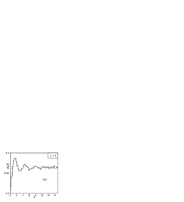
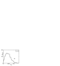
FIG. 1.: Microscopic spectral density (left) and distribution of the smallest eigenvalue (right) of the staggered Dirac operator in quenched SU(3) for $\beta=5.4$ and $V=L^{4}$ with $L=4$, 6, 8, 10. The histograms represent the lattice data, the dashed curves are the predictions of Eqs. (8) (with $\mu=0$) and (9).

In Eq. (8), we have used $\mu=0$. Clearly, $N_{f}=0$ since we consider the quenched approximation. The fact that $\nu=0$ is less obvious. The prediction of Eq. (8) is restricted to sectors with definite topological charge. Therefore, one should compute the topological charge of each gauge field configuration and compare the lattice data in each topological sector with the prediction of Eq. (8). However, Eq. (8) assumes that for $\nu\neq 0$ the Dirac operator has exact zero modes. This is not the case for staggered fermions on the lattice where at finite lattice spacing $a$ the would-be zero modes are shifted by an amount proportional to $a^{2}$ [19]. For the value of $\beta$ we used, $a$ is still relatively large so that no zero modes are present. This explains why the lattice data are consistent with Eq. (8) for $\nu=0$, as seen in Fig. 1. Very similar results for different $\beta$ were very recently presented in [14].

The agreement between the lattice data and the universal predictions is quite satisfactory, also for the two-point cluster function in the microscopic limit which we have plotted in Fig. 2 along with the prediction of Eq. (10) for $\mu=0$.

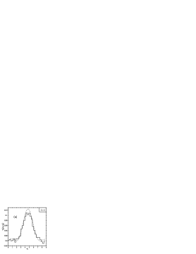
FIG. 2.: Microscopic two-point cluster function $\tau_{2}(z_{1},z_{2})$ with $z_{2}$ at the second maximum of $\rho_{s}(z)$ for $L=4$ and $L=6$, respectively. The histograms represent the lattice data, the dashed curves are the prediction of Eq. (10) for $\mu=0$.

A fixed value of $z_{2}=4.68$ (corresponding to the location of the second maximum of $\rho_{s}(z)$) was chosen.

The quantity $\tau_{2}(z_{1},z_{2})$ is interesting since it enters in the calculation of the disconnected scalar susceptility which, in turn, can be used to determine the Thouless energy, i.e., the scale $\lambda_{\mathrm{RMT}}$ above which the lattice data deviate from the universal predictions of Eqs. (8) through (10). In terms of the Dirac eigenvalues, this quantity is defined as [20]

$$\chi^{\mathrm{disc}} = \frac{1}{V}\left\langle\sum_{k,\ell=1}^{N}\frac{1}{(i\lambda_{k}+m)(i\lambda_{\ell}+m)}\right\rangle$$ (13)

$$\mbox{}-\frac{1}{V}\left\langle\sum_{k=1}^{N}\frac{1}{i\lambda_{k}+m}\right\rangle^{2}\>,$$

where $V$ is the number of lattice sites, $N$ the number of eigenvalues and $m$ a valence quark mass, respectively. The average is over independent gauge field configurations. Eq. (13) can be rewritten in terms of integrals involving the spectral one- and two-point functions of the Dirac operator. Rescaling $\chi^{\mathrm{disc}}$ by $1/(V\Sigma^{2})$ and changing from $m$ to $u=mV\Sigma$, we have

$$\chi^{\mathrm{disc}}(u) = 4u^{2}\int_{0}^{\infty}dx\>\frac{\rho_{s}(x)}{(x^{2}+u^{2})^{2}}$$ (15)

$$\mbox{}-4u^{2}\int_{0}^{\infty}\int_{0}^{\infty}dxdy\>\frac{\tau_{2}(x,y)}{(x^{2}+u^{2})(y^{2}+u^{2})}$$

$$= -u^{2}[K_{\mu}^{2}(u)-K_{\mu+1}(u)K_{\mu-1}(u)]$$ (17)

$$\quad\times[I_{\mu}^{2}(u)-I_{\mu+1}(u)I_{\mu-1}(u)]\>,$$

where in going from the first to the second line we have inserted the RMT results for $\rho_{s}$ and $\tau_{2}$. The functions $I$ and $K$ are modified Bessel functions. In the case of $\mu=0$, Eq. (15) simplifies to

$$\chi^{\mathrm{disc}}(u)=u^{2}\bigl{[}K_{1}^{2}(u)-K_{0}^{2}(u)\bigr{]}\bigl{[}I_{0}^{2}(u)-I_{1}^{2}(u)\bigr{]}\>.$$ (18)

In order to compare the lattice results for $\chi^{\mathrm{disc}}$ obtained from Eq. (13) with the RMT prediction of Eq. (15) we introduce the variable [15]

$$\mathrm{ratio}=\frac{\chi^{\mathrm{disc}}_{\mathrm{lattice}}-\chi^{\mathrm{disc}}_{\mathrm{RMT}}}{\chi^{\mathrm{disc}}_{\mathrm{RMT}}}$$ (19)

which is plotted in Fig. 3.

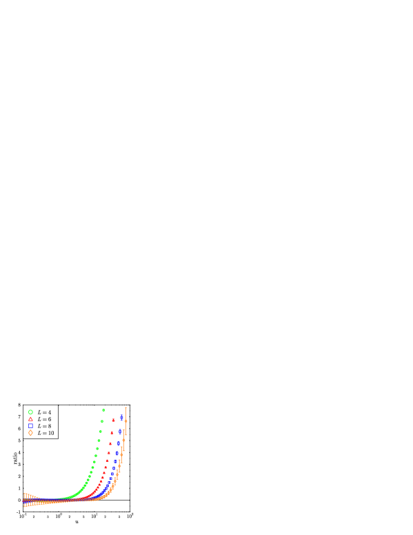
FIG. 3.: The ratio defined in Eq. (19) for $\beta=5.4$ and various lattice sizes.

This ratio should be close to zero in the domain of validity of the RMT predictions and deviate from zero at some value of $u=u_{\mathrm{RMT}}$ which corresponds to the Thouless energy. (The deviations of the ratio from zero for very small values of $u$ are artefacts of the finite lattice size and of finite statistics. This point was discussed in Ref. [15].)

The prediction of Eq. (2) is that $\lambda_{\mathrm{RMT}}/\Delta$ should scale with $L^{2}$. If we express $\lambda_{\mathrm{RMT}}$ in terms of $u_{\mathrm{RMT}}=\lambda_{\mathrm{RMT}}V\Sigma=\pi\lambda_{\mathrm{RMT}}/\Delta$, $u_{\mathrm{RMT}}$ should also scale with $L^{2}$. To check this predicted scaling behavior we have plotted the ratio of Eq. (19) as a function of $u/L^{2}$ in Fig. 4.

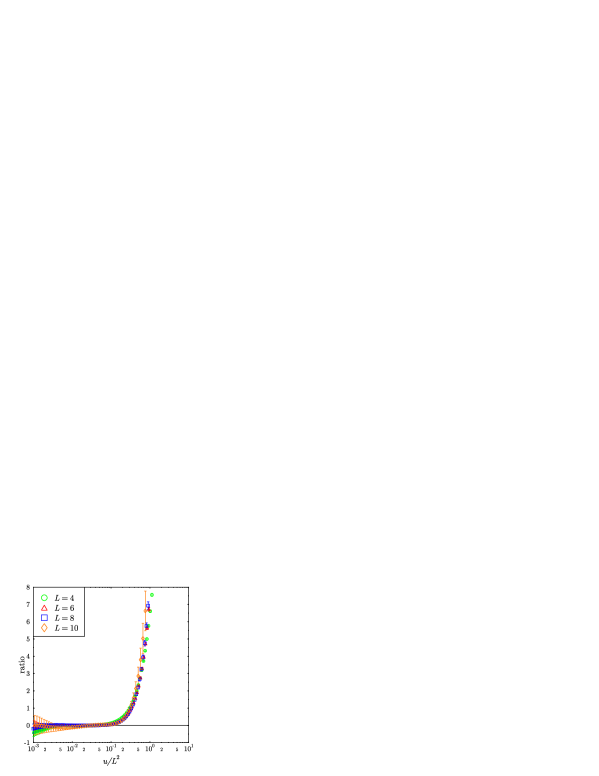
FIG. 4.: The ratio of Eq. (19) plotted versus $u/L^{2}$.

We observe that all data fall on the same curve, confirming the prediction of Eq. (2) with regard to the scaling with $L^{2}$. Since we have only considered one value of $\beta$, we cannot check the scaling with $f_{\pi}^{2}$. From Fig. 4 we can read off $\lambda_{\mathrm{RMT}}/\Delta\approx 0.04L^{2}$ in lattice units.

In summary, we have shown that the distribution and the correlations of the low-lying eigenvalues of the staggered Dirac operator in quenched SU(3) are described by universal functions up to a certain energy scale, the Thouless energy. The latter quantity was determined using the disconnected scalar susceptibility, and the predicted scaling with $L^{2}$ was confirmed. It would be of great interest to extend the present study to dynamical fermions for which analytical results are also available [21].

Acknowledgments. We thank S. Meyer and H.A. Weidenmüller for helpful discussions. This work was supported in part by DFG grants Scha-458/5-2 and We-655/15-1.

REFERENCES

- [1] T. Banks and A. Casher, Nucl. Phys. B169, 103 (1980).
- [2] H. Leutwyler and A.V. Smilga, Phys. Rev. D 46, 5607 (1992).
- [3] E.V. Shuryak and J.J.M. Verbaarschot, Nucl. Phys. A560, 306 (1993).
- [4] J.J.M. Verbaarschot and I. Zahed, Phys. Rev. Lett. 70, 3852 (1993).
- [5] J.C. Osborn, D. Toublan, and J.J.M. Verbaarschot, hep-th/9806110.
- [6] R.A. Janik, M.A. Nowak, G. Papp, and I. Zahed, Phys. Rev. Lett. 81, 264 (1998).
- [7] J.C. Osborn and J.J.M. Verbaarschot, Phys. Rev. Lett. 81, 268 (1998); Nucl. Phys. B525, 738 (1998).
- [8] J. Stern, hep-ph/9801282.
- [9] M.E. Berbenni-Bitsch, S. Meyer, A. Schäfer, J.J.M. Verbaarschot, and T. Wettig, Phys. Rev. Lett. 80, 1146 (1998).
- [10] J.-Z. Ma, T. Guhr, and T. Wettig, Euro. Phys. J. A 2, 87 (1998).
- [11] M.E. Berbenni-Bitsch, S. Meyer, and T. Wettig, Phys. Rev. D 58, 071502 (1998).
- [12] P.H. Damgaard, U.M. Heller, A. Krasnitz, and T. Madsen, hep-lat/9803012.
- [13] F. Farchioni, I. Hip, C.B. Lang, and M. Wohlgenannt, hep-lat/9809049.
- [14] P.H. Damgaard, U.M. Heller, and A. Krasnitz, hep-lat/9810060.
- [15] M.E. Berbenni-Bitsch, M. Göckeler, T. Guhr, A.D. Jackson, J.-Z. Ma, S. Meyer, A. Schäfer, H.A. Weidenmüller, T. Wettig, and T. Wilke, Phys. Lett. B 438, 14 (1998).
- [16] J.J.M. Verbaarschot, Phys. Rev. Lett. 72, 2531 (1994).
- [17] P.J. Forrester, Nucl. Phys. B402, 709 (1993).
- [18] M. Creutz, Phys. Rev. D 36, 515 (1987).
- [19] J.C. Vink, Phys. Lett. B 210, 211 (1988).
- [20] J.J.M. Verbaarschot, Phys. Lett. B 368, 137 (1996).
- [21] P.H. Damgaard and S.M. Nishigaki, Nucl. Phys. B518, 495 (1998); T. Wilke, T. Guhr, and T. Wettig, Phys. Rev. D 57, 6486 (1998); G. Akemann and P.H. Damgaard, Phys. Lett. B 432, 390 (1998); B. Seif, T. Wettig, and T. Guhr, hep-th/9811044.