Abstract

We discuss the spectrum of hadrons with a heavy colour-adjoint particle - motivated by the gluino of supersymmetry. Using the lattice approach, we explore in detail the gluonic bound states - the ‘glueballino’ or ‘gluelump’. We also make a first determination of the spectrum of the ‘adjoint mesons’ - which have a light quark and antiquark bound to the heavy adjoint particle. A comparison of the spectra of these two systems is also made.

1 Introduction

It is possible to explore the bound states in QCD of a particle with adjoint colour. This is of interest for comparison with phenomenological models. For a pioneering study see ref. [1] which used the MIT bag model. It may also be of relevance to experiment should a massive gluino ($\tilde{g}$) exist which is sufficiently stable to form hadronic bound states. These colour-singlet hadrons containing a gluino have been called ‘R-hadrons’ [2]. They include the bound states of a gluino and gluons, $g\tilde{g}$ referred to as a ‘glueballino’. Another possibility is an R-meson, a $\tilde{g}q\bar{q}$ system, which might also be referred to as the ‘hybridino’ from its relationship to the $gq\bar{q}$ hybrid meson. The R-baryon is a $\tilde{g}qqq$ system and it is possible that the $\tilde{g}uds$ state might be the lightest of the R-hadrons [3]. It has been proposed [4] that these R-hadrons may have astrophysical significance as components of cosmic rays and, in this case, the mass differences between different R-hadrons play a crucial role in determining whether the appropriate states could be stable.

A non-perturbative study of these states from first principles is possible by using numerical lattice techniques. In this case, it is convenient to treat the gluino in the heavy-gluino limit. This will be appropriate if the gluino mass is large compared to the QCD scale of order 1 GeV. In this limit, the fermionic nature of the gluino will be irrelevant and one can use a static adjoint source. In this context, the gluonic bound states are known as the ‘gluelump’ [5], while we choose to call the quark-antiquark bound states the ‘adjoint meson’. We will be unable to address the issue of the spectrum of ‘adjoint baryons’.

We use quenched lattices to explore the spectrum of the gluelump. This has been studied previously [5] but only limited results exist for SU(3) colour [6]. A preliminary version of our work has been presented elsewhere [7]. Here we make a thorough study of many $J^{PC}$ states and we extract the continuum limit of the mass differences between the lower lying states.

The adjoint mesons have not been studied previously on a lattice. One reason is that, because the heavy adjoint particle does not propagate spatially, the light quark propagators are only needed at the same spatial sink as source. This feature, common to studies of B-mesons and the $\Lambda_{b}$ baryon, means that conventional light quark propagator methods are very inefficient. A promising new method allows the relevant light quark propagators to be evaluated from nearly all sources to nearly all sites [8]. This has been used successfully for static quarks and here we use similar methods to tackle static adjoint particles. Our study is exploratory and we will not be able to remove completely the systematic errors associated with lattice methods: extrapolation to light quarks, continuum limit extrapolation, etc. We also use quenched lattices which inherently implies at least a 10% systematic error from setting the scale.

2 The Gluelump Spectrum

We explore here bound states of the static adjoint source in the presence of the gluonic degrees of freedom. This has been explored previously in lattice studies [5, 6, 9] and we use similar techniques.

For a heavy gluino of zero velocity, one can ignore the gluino spin and treat the propagation in the time direction as a product of adjoint gauge links. This approach, as is the case for heavy quarks in the static limit, trades a dependence on the heavy particle mass for a lattice self-energy which diverges as the lattice spacing $a$ is taken to zero. Thus we will only be able to compare with physical predictions for the difference of masses between states with the same adjoint particle content. This is, however, entirely sufficient for our purposes.

For the adjoint gauge links, we use the real $8\times 8$ adjoint matrices related to their fundamental counterparts by

$$U_{4}^{{\rm Adj\ }\alpha\beta}={1\over 2}{\rm Tr}(U_{4}{\lambda^{\alpha}}U_{4}^{\dagger}{\lambda^{\beta}})$$ (1)

where the $\lambda$-matrices are the conventional ones. For propagation of the static adjoint source, we need the time-directed product of these links.

$$G^{A}=\prod U_{4}^{\rm Adj}$$ (2)

Figure 1: The gauge links involved in a gluelump correlation.

To create and destroy the gluelump states we use products of fundamental gauge links ($U_{G}$) which start and finish on the adjoint source site. The schematic method is illustrated in fig. 1. We choose operators that are in irreducible representations of $O_{h}$ to explore the spin structure of the gluelump states. In the continuum limit, states of the gluonic field are labelled by $J^{PC}$. We relate continuum spins to those obtained from the $O_{h}$ subgroup by subduction. Note that the bound states of an actual gluino (the glueballino) will be fermions, but in the limit of a heavy gluino, the gluino spin is uncoupled so that our study gives all the relevant information.

For speed of computation, we chose to build the gluonic operators out of square elements. From these we construct ‘clover like’ operators from various sums of these squares, projected onto the adjoint representation with definite charge conjugation:

$$H^{\alpha}={\rm Tr}(\lambda^{\alpha}U_{G}\pm\lambda^{\alpha}U_{G}^{\dagger})$$ (3)

The coefficients for creating given $O_{h}$ representations can be determined from the projection table given in [10]. In choosing the planar square as the building block, we are only able to access 10 out of a possible 20 $O^{PC}$ representations. However, we expect the lower energy states to be created by such planar constructs.

The correlation of interest is then given by evaluating $H^{\alpha}G^{A}_{\alpha\beta}H^{\beta}$. Diagrammatically the correlation in a typical group representation looks like that in fig. 1.

Measurement of objects containing static propagators is hampered by cumulative statistical errors from multiplying links, each with a variance $O(1)$. Adjoint links are even more sensitive to this effect [11]. In order to make effective measurements at larger times where the excited state contributions are minimised, we employ a link integration or multi-hit technique [12] which involves summing time-oriented links over a set of independently generated alternatives provided by performing a local heatbath algorithm on them. The force term is generated by the surrounding gauge links or ‘staples’ from the original gauge configuration. We choose to use 10 or 15 samples of the time-directed link with this force separated by 3 Cabibbo-Marinari SU(2) subgroup updates and then construct the average of the adjoint links obtained from each of them.

We measure correlations for a given state using four operators at both source and sink. These were constructed using two sizes of square built from products of fuzzed links with the fuzzing algorithm performed to two different numbers of iterations. Each iteration of the fuzzing algorithm makes a gauge invariant replacement of a link, $U_{\mu}(x)$, according to a sum over 4 staples:

$$U_{\mu}(x)\rightarrow P_{SU(3)}\left(CU_{\mu}(x)+\sum U_{\nu}(x)U_{\mu}(x+\hat{\nu})U_{\nu}^{\dagger}(x+\hat{\mu})\right)~{}$$ (4)

where $P_{SU(3)}$ is a projection into the SU(3) group. The fuzzing parameters, and square sizes were tuned according to the lattice spacing to give the best signal. We measured correlations from all sites and time planes on various quenched lattices, as shown in Table 1. The interpolation of $r_{0}$ values we used is also given for completness.

We then employed the variational technique on the $4\times 4$ matrix of correlations in order to determine the linear combination of operators which maximises the ground state contribution. In practice, since statistical errors increase with time separation $t$, we determined the basis for the ground state from a moderate $t$ separation ($t=1$ to $t=0$) and then explored the $t$-dependence of that combination to larger $t$. Since the effective mass should decrease monotonically with increasing $t$ to the ground state mass, we seek to find the level of the plateau. Since the statistical error increases with $t$, a sensible prescription is to select the mass from the $t$ values beyond which the data are consistent with such a plateau. We are also able to obtain estimates of the energies of excited states from the variational approach.

Table 1: Lattices used in the gluelump calculation

$\beta$	Size	Number	Square sizes	$C$	Fuzzing iterations	$r_{0}$
		of lattices
5.7	$12^{3}\times 24$	99	1,2	4.0	10,20	2.940
6.0	$16^{3}\times 48$	202	2,3	4.0	20,30	5.272
6.2	$24^{3}\times 48$	60	2,3	4.0	30,45	7.319

In Table LABEL:tab:glefmass we present the lattice effective masses from adjacent $t$-values in the optimum variational basis, where such determination was statistically significant. We also give some results for the first excited states. We compare our results with an earlier exploratory calculation of the gluelump spectrum  [6] based on 50 $\beta=5.7$ lattices. The measurement of the $T_{1}^{+-}$ and $T_{1}^{--}$ masses were given as 2.046(89) and 2.096(89) at $t=3:2$ respectively. These older results are seen to have the ordering we find but to underestimate the mass splitting.

Table 2: Gluelump masses (ground state and first excited state in some cases) for different $O_{h}$ representations in lattice units.

$O^{PC}$	$\beta$	$t=2:1$	$t=3:2$	$t=4:3$	$t=5:4$
$T_{1}^{+-}$	5.7	1.845(6)	1.813(15)	1.811(48)	1633(169)
		2.506(1)	2.354(92)
	6.0	1.339(3)	1.329(5)	1.326(5)	1.330(8)
		1.736(3)	1.690(6)	1.683(17)	1.650(53)
	6.2	1.152(2)	1.142(3)	1.145(3)	1.146(9)
		1.469(3)	1.445(7)	1.446(11)	1.429(27)
$T_{1}^{--}$	5.7	2.101(8)	2.006(33)	2.078(123)
		2.709(37)	2.284(201)
	6.0	1.505(2)	1.486(4)	1.486(8)	1.495(21)
		1.883(4)	1.829(10)	1.779(28)	1.674(93)
	6.2	1.276(3)	1.261(5)	1.247(8)	1.249(12)
		1.587(4)	1.534(7)	1.532(21)	1.446(56)
$T_{2}^{--}$	5.7	2.242(10)	2.280(45)	2.155(310)
		2.740(29)
	6.0	1.593(2)	1.579(4)	1.549(10)	1.557(30)
		1.946(4)	1.892(10)	1.900(42)	1.874(145)
	6.2	1.347(3)	1.331(7)	1.322(14)	1.296(17)
		1.646(4)	1.609(8)	1.570 (26)	1.502(107)
$E^{+-}$	5.7	2.470(18)	2.230(80)	1.862(465)
	6.0	1.759(3)	1.735(8)	1.744(22)	1.683(78)
	6.2	1.469(4)	1.452(9)	1.451(23)	1.426(41)
$A_{2}^{+-}$	5.7	2.542(26)	3.023(347)
	6.0	1.779(4)	1.775(13)	1.684(33)	1.667(114)
	6.2	1.499(6)	1.477(9)	1.460(28)	1.399(43)
$A_{1}^{++}$	5.7	2.628(47)
	6.0	1.786(5)	1.762(16)	1.721(48)	1.836(157)
	6.2	1.502(7)	1.457(15)	1.474(41)	1.539(92)
$E^{++}$	5.7	2.897(50)
	6.0	1.936(6)	1.883(16)	1.927(60)
	6.2	1.603(6)	1.575(14)	1.563(28)	1.556(91)
$T_{1}^{-+}$	5.7	2.900(37)
	6.0	1.966(4)	1.918(14)	1.918(45)
	6.2	1.641(5)	1.613(11)	1.599(34)	1.488(45)
$T_{2}^{-+}$	5.7	3.131(49)
	6.0	2.085(5)	2.053(18)	2.216(104)
	6.2	1.727(5)	1.698(18)	1.683(46)	1.661(111)
$T_{2}^{++}$	5.7	3.144(52)
	6.0	2.148(5)	2.130(18)	2.142(98)
	6.2	1.788(6)	1.700(20)	1.749(81)

Figure 2 shows the spectrum of states calculated at $\beta=6.0$. The points marked with circles are the lowest eigenvalues from the ten measured representations. They are plotted against $J$ assuming the lowest spin contained in the $O_{h}$ representation. We also determine some higher energy eigenvalues for each $O_{h}$ representation we study. These could either be radial excitations with the lowest spin assignment or could be in a higher spin representation allowed by that $O_{h}$ representation (for example $T_{1}^{+-}$ can be $J^{PC}=1^{+-}$ or $3^{+-}$). In principle a thorough study of all eigenvalues in all $O_{h}$ representations in the continuum limit will allow the $J^{PC}$ values to be assigned unambiguously. In the present application, we have used a solid triangle to show plausible assignments of $J$ for these excited states. We see that in our $4\times 4$ basis these energy eigenvalues qualitatively agree with the expected degeneracies in the continuum spectrum (for example a $J=3$ state has $T_{1}$, $T_{2}$ and $A_{2}$ degenerate levels).

As found previously [6], the $J^{PC}=1^{+-}$ and $1^{--}$ states are lowest lying. Surprisingly, the lightest $0^{++}$ state is considerably heavier. Since the overall lattice energy contains an unphysical self-energy, we examine mass differences between states for each lattice spacing. To determine a continuum estimate, we study a dimensionless quantity choosing $r_{0}(a)$ ($r_{0}$ is defined from the force between static quarks as $F(r_{0})r_{0}^{2}=1.65$, corresponding to about 0.5 fm, and it is measured accurately [13, 14] on a lattice from the static potential) to set the scale of the measured lattice mass differences $M$. Then we perform a linear fit to $M(a)r_{0}(a)$, against $r_{0}(a)^{-2}$ since, in the quenched approximation, lattice corrections are of order $a^{2}$. The data are illustrated in figure 3 (which also shows some additional low statistics results from $\beta=5.9$). We thus obtain an estimate of the continuum limit mass splittings. The results for the lowest few states are shown in Table 3 where the results quoted in MeV have an additional overall scale error of 10% coming from the quenched approximation scale. We also show the most plausible assignment of the spin in the continuum limit. One rather surprising feature is the observed degeneracy of the $A_{2}^{+-}$ and $E^{+-}$ states - this is not compatible with a single common spin assignment, so we have assigned the lowest spin option in each case.

In the continuum limit we expect the $O_{h}$ representations to group into degenerate levels with the rotational symmetry restored. Thus for any $J$ assignment of a $E^{++}$ state (for example $J=2$ or 4), there should be associated a degenerate $T_{2}^{++}$ state in the continuum limit. Our results show that the lightest $E^{++}$ is not accompanied by such a degenerate $T_{2}{++}$ state at $\beta=6.0$ or at $\beta=6.2$. We do find, however, that the mass difference in units of $r_{0}$ between the $E^{++}$ and $T_{2}^{++}$ is consistent, within statistical errors, with decreasing (like $a^{2}$) to zero in the continuum limit. This suggests that the lattice artefact errors (for instance those discussed here from lack of rotational invariance) may be relatively sizeable for these higher lying states. This conclusion is also supported by Figure 3 which shows a stronger $a^{2}$ dependnce for heavier states.

Figure 2: Gluelump Spectrum at $\beta=6.0$

Figure 3: The $O^{PC}-T_{1}^{+-}$ gluelump mass splitting in units of $r_{0}$ versus $a^{2}$ in units of $r_{0}$. The continuum limit is at the left and a straight line behaviour is expected for small $a$.

Table 3: Continuum Limit estimation of the $O^{PC}-T_{1}^{+-}$ mass splitting.

State	J	$\Delta(Mr_{0})_{a=0}$	Energy(MeV)	$\chi^{2}/{\rm dof}$
$T_{1}^{--}$	1	0.933(18)	368(7)	0.874
$T_{2}^{--}$	2	1.438(25)	584(10)	1.749
$E^{+-}$	2	2.467(92)	973(36)	0.312
$A_{2}^{+-}$	3	2.468(60)	972(24)	0.113
$A_{1}^{++}$	0	2.771(72)	1092(28)	0.137

2.1 Potentials as $R\to 0$

There is a correspondence between the gluelump energies we have just determined and the limit of excited gluonic potentials as $R\to 0$. This has been noted before [5]. Here we are in a position to explore the consequences of this relationship more fully since we have determined the gluelump spectrum in detail.

The potential between fundamental colour sources at separation $R$ has been widely studied. Of special interest are the gluonic excitations of this potential - corresponding to excited energy levels [15, 16, 17]. In the limit as $R\to 0$, the static source and anti-source will be at the same site and hence their colour can be combined in a gauge invariant way - creating a singlet and an adjoint colour source. This latter is just the situation we study here: the gluelump is an adjoint source in the presence of a gluonic field, while the colour singlet correlation is given glueball exchange (plus a vacuum contribution when the $J^{PC}$ representation of the object created is $0^{++}$).

Thus for the generalised Wilson loop in the limit of zero spatial separation, we have

$$\lim_{R\to 0}W(R,t)=ce^{-M_{\rm gluelump}t}+c^{\prime}e^{-M_{\rm glueball}t}$$ (5)

In the large $t$ limit, the lighter of the two states will dominate the correlation function. In most cases of present interest, the gluelump state is lighter than the glueball. We can obtain a relationship between the gluonically-excited states of the generalised Wilson loop, in the limit $R\to 0$, and those measured in the gluelump spectrum. This relationship in the continuum is obtained by subducing the SU(2) representations appropriate to the gluelump to the $D_{\infty h}$ representations appropriate to the generalised Wilson loop when $R\neq 0$. The latter representations are labelled for $J_{z}=0$, 1 ,2 as $\Sigma$, $\Pi$, $\Delta$ where $z$ is the axis of separation of the fundamental sources which are $R$ apart. The other labels of the representations are $g,\ u$ for $CP=\pm 1$ and, for the $\Sigma$ states only, an additional $\pm$ label indicating whether the sate is even/odd under reflection in the plane containing the $z$-axis. By subducing the irreducible representation of the gluelump with $J^{PC}$ we will find $D_{\infty h}$ representations with $J_{z}=-J,\dots,J$; labels $g,\ u$ given by $CP$ and, for any $J_{z}=0$ states, an additional label given by $P(-1)^{J}$. These relationships are tabulated in Table  4.

The same identities as $R\to 0$ also apply explicitly to the lattice discretisation. Then the $O_{h}$ representations appropriate for the gluelump can be subduced into the $D_{4h}$ representations appropriate for the generalised Wilson loop with $R\neq 0$. Thus, as has been emphasised previously [5], the ground state gluelump with $1^{+-}$ ($T_{1}^{+-}$) implies that as $R\to 0$ there must be a degeneracy of the two-dimensional $\Pi_{u}$ state ($E_{u}$) and a $\Sigma_{u}^{-}$ state ($A_{1u}$).

Although the above group-theoretical identities are a good guide to the behaviour of the excited gluonic potentials at small $R$, the limit as $R\to 0$ of the excited gluonic potential is not trivial to extract from lattice data with $R=a,\ R=2a,\dots$. One guide is to consider the gluon exchange contributions perturbatively. A way to investigate this is to consider the self energies of the contributions: $2E_{F}$ at $R\neq 0$ and $E_{A}$ at $R=0$, where $F$ and $A$ label fundamental and adjoint colours. Since, to lowest order, $E_{A}=9E_{F}/4$ for SU(3) of colour, there will be a mismatch and one might expect the energy to increase as $R\to 0$ since the adjoint self-energy is larger. Another way to investigate this, is to imagine that as $R\approx 0$, there is a gluonic field in the adjoint representation, so that the heavy quark and anti-quark are also in an adjoint and hence will have a Coulombic interaction energy given by $-1/8$ of the Coulombic energy between a quark and antiquark in the fundamental representation (which is approximately given by $-0.25/R$ in lattice quenched studies). This again suggests that the excited gluonic potential should rise as $R\to 0$, here as $0.03/R$.

Lattice data for the $E_{u}$ representation for small $R$ from SU(2) colour studies [18] at $\beta=2.4$ with values of $aV_{Eu}(R)=1.31$, 1.32 and 1.38 for $R=3a,\ 2a$ and $a$ respectively do qualitatively support these estimates of the small $R$ behaviour of the excited gluonic potential and are consistent with a limit as $R\to 0$ which agrees with the lattice gluelump energy [9] of $aE_{\rm gluelump}=1.50$. Also in fig. 4, we show the comparison of the small $R$ excited gluonic potentials at $\beta=6.2$ with our SU(3) gluelump analysis, where both results use the same Wilson lattice regularisation and so are directly related. This figure confirms the degeneracy of the excited gluonic energy levels as $R\to 0$ with a common value given by the appropriate gluelump energy, as we found above.

These considerations are useful [19] to understand the extensive results on the spectrum of excited gluonic levels that have been determined recently [17].

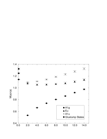
Figure 4: The static quark potential energy in units of $r_{0}$ at $\beta=6.2$ from ref.[16] for the ground state ($A_{1g}$) and excited gluonic states ($E_{u}$ and $A_{1u}$) versus separation $R$ in lattice units. The leftmost points are (in increasing energy) the gluelump energies for $T_{1}^{+-}$, $T_{1}^{--}$ and $T_{2}^{--}$ representations. This illustrates the expected degeneracy at $R=0$ between the two excited gluonic states which must both equal the lowest gluelump energy.

Table 4: Connection between gluelump and two-body potential as $R\to 0$.

Gluelump $J^{PC}$	Two-body potential states
$1^{+-}$	$\Pi_{u}$, $\Sigma_{u}^{-}$
$1^{--}$	$\Pi_{g}$, $\Sigma_{g}^{+}$
$2^{--}$	$\Pi_{g}$, $\Sigma_{g}^{-}$, $\Delta_{g}$

3 The Adjoint-meson spectrum

The state with a static adjoint source bound to a quark and antiquark is now studied. We refer to this as the adjoint-meson and label the states by the $J^{PC}$ of the quark anti-quark subsystem but with a suffix $A$ to indicate the adjoint source. In the context where the adjoint source is considered to be an approximation to a heavy gluino, such a bound state has also been called the R-meson [2] and might logically be called a hybridino since it is the supersymmetric partner of a hybrid meson. Note that the bound states of a gluino will actually be fermions, but in the limit of a heavy gluino, the gluino spin is irrelevant and the study with a bosonic adjoint source gives the required information.

The lattice adjoint-meson is generated by coupling the static adjoint source to a light quark-antiquark system. As for the case of B meson studies (and those of the $\Lambda_{b}$ baryon), much improved statistics are available if one can evaluate the light quark propagators from all sites as sources. This can be achieved using stochastic propagators [8].

The stochastic inversion is based on the relation:

$$G_{ij}={\cal M}_{ij}^{-1}=\frac{1}{Z}\int{\cal D}\phi\;({\cal M}_{jk}\phi_{k})^{\ast}\phi_{i}\;\exp\left(-\phi_{i}^{\ast}({\cal M}^{\dagger}{\cal M})_{ij}\phi_{j}\right)$$ (6)

where, in our case, ${\cal M}$ is the clover-improved Wilson-Dirac fermionic operator and the indices $i,j,k$ represent simultaneously the space-time coordinates, the spinor and colour indices. For every gauge configuration, an ensemble of independent fields $\phi_{i}$ (we use 24 following [8]) is generated with gaussian probability:

$$P[\phi]=\frac{1}{Z}\exp\left(-\phi_{i}^{\ast}({\cal M}^{\dagger}{\cal M})_{ij}\phi_{j}\right)$$ (7)

All light propagators are computed as averages over the pseudo-fermionic samples:

$$G_{ij}=\left\{\begin{array}[]{l}\langle({\cal M}\phi)_{j}^{\ast}\phi_{i}\rangle\\ \mathrm{or}\\ \gamma_{5}\langle\phi_{j}^{\ast}({\cal M}\phi)_{i}\rangle\gamma_{5}\end{array}\right.$$ (8)

where the two expressions are related by $G_{ij}=\gamma_{5}G_{ji}^{\dagger}\gamma_{5}$. Moreover, the maximal variance reduction method is applied in order to minimise the statistical noise [8]. The maximal variance reduction method involves dividing the lattice into two boxes ($0<t<T/2$ and $T/2<t<T$) and solving the equation of motion numerically within each box, keeping the pseudo-fermion field $\phi$ on the boundary fixed. According to the maximal variance reduction method, the fields which enter the correlation functions must be either the original fields $\phi$ or solutions of the equation of motion in disconnected regions. The stochastic propagator is therefore defined from each point in one box to every point in the other box or on the boundary. Hadronic correlators are then evaluated with the hadron source and sink in different boxes. In order to implement this requirement, we only evaluate correlators for $t\geq 2$. For further details, see see Michael and Peisa [8], especially their application to the $\Lambda_{b}$ meson. Note that, in any method which involves solving the lattice Dirac equation, it is not consistent to use multihit improvement for the time-directed gauge links.

We construct creation operators for the adjoint quark bilinear according to,

$${\cal H}^{\alpha}_{\rm Adj}=\bar{\psi}(x)\lambda^{\alpha}\Gamma\psi(x)$$ (9)

such that the correlation function is given by combining this with the static adjoint source $G^{A}$, defined previously, and replacing quark propagator terms, $\bar{\psi}_{i}\psi_{j}$ as $\langle\phi_{j}({\cal M}_{ik}\phi_{k})^{*}\rangle$ as described above. The correlation function is given by

$$C(\Gamma,t_{2}-t_{1}) = \sum_{x}\left(\bar{\psi}(x,t_{1})\lambda^{\alpha}\Gamma\psi(x,t_{1})\right)^{\dagger}G^{A}_{\alpha\beta}(x,t_{1},t_{2})\bigl{(}\bar{\psi}(x,t_{2})\lambda^{\beta}\Gamma\psi(x,t_{2})\bigr{)}$$ (10)

$$= {1\over N_{s}(N_{s}-1)}\sum_{x}\sum_{i\neq j}{\rm Tr}_{\rm(fund)}\bigl{(}\phi_{j}(x,t_{1})\lambda^{\alpha}\Gamma({\cal M}\phi_{i})^{*}(x,t_{1})$$

$$\times \phi_{i}(x,t_{2})\lambda^{\beta}\Gamma({\cal M}\phi_{j})^{*}(x,t_{2})\bigr{)}G^{A}_{\alpha\beta}(x,t_{1},t_{2})$$

where $i$ and $j$ are different samples of the $N_{s}$ pseudofermion fields. We symmetrise the placement of $t_{1}$ and $t_{2}$ about the boundaries of the stochastic source at $t=0$ or $T/2$. Where $t_{2}-t_{1}$ is odd we average over the two possible placements.

Table 5: Lattices used in the adjoint-meson calculation

$\beta$	Lattice	Propagator	$\kappa$	$C_{SW}$	Gauge	$M_{P}$	$M_{V}$
	size	samples			configs.
5.7	$8^{3}\times 16$	24	0.13843	1.57	20
5.7	$12^{3}\times 24$	24	0.13843	1.57	20	0.736(2)	0.938(3)
5.7	$8^{3}\times 16$	24	0.14077	1.57	20
5.7	$12^{3}\times 24$	24	0.14077	1.57	20	0.529(2)	0.815(5)
6.0	$16^{3}\times 24$	24	0.13714	1.76	10	0.309(2)	0.488(5)

We measure the correlation for observables with $\Gamma=\gamma_{5},\ \gamma_{i}$ and $I$, corresponding to $P_{A},\ V_{A}$ and $S_{A}$ (scalar) mesons, respectively, averaging over the components of $\gamma_{i}$ for the $V_{A}$ case. Other $J^{PC}$ combinations were found to be more poorly determined with masses comparable to the scalar case, $S_{A}$, or higher.

Because the stochastic inversion method evaluates so many samples of the correlation from each gauge configuration, it is feasible to obtain results from moderate numbers of gauge configurations. The lattices used are detailed in Table 5. At $\beta=5.7$ we use the parameters for tadpole-improved clover fermions studied previously [20]. With two values of the hopping parameter, the lighter of which corresponds approximately to the strange quark mass, we are able to explore the dependence on $\kappa$ of the spectrum and the extrapolation to the chiral limit. We also evaluated stochastic propagators at $\beta=6.0$ with NP-improved clover fermions to be able to explore the lattice spacing dependence. The masses of the pseudoscalar and vector mesons quoted in Table 5 come from previous studies [20, 21] using conventional propagators for these lattice parameters.

We construct isotropic extended (fuzzed) operators by replacing the light quark fields using

$$\psi_{l}(x)^{\mathrm{fuzzed}}=\Sigma_{\pm(\mu=1,3)}{U^{(l)}_{\mu}(x)\psi(x+la_{\mu})}$$ (11)

where $U_{-\mu}(x)=U^{\dagger}_{\mu}(x-\hat{\mu})$ in this context. Here $U^{(l)}$ is a product of fuzzed links in a straight line of length $la$, each link defined according to Equation 4. At $\beta=5.7$ we explored two choices of fuzzing, namely 2 iterations with $C=2.5$ and 12 iterations with $C=4.0$, each with links of length one in eq. 11. The smaller number of fuzzing iterations gave a more accurate value for the correlations and this was chosen for the $12^{3}$ spatial lattice for the $V_{A}$ and $P_{A}$ studies. For $\beta=6.0$, we used 6 iterations of fuzzing with $C=2.5$ but used links of length 2. By replacing in Equation 10 with fuzzed operators all the $\phi$ fields at $t_{1}$ or at $t_{2}$ or at both ends, we generate a $2\times 2$ correlation matrix.

As in the gluelump case, we performed a variational analysis on the data to obtain estimates of the ground state mass. Because the excited state contributions are relatively large, we use $t$-values of 3 and 4 to establish the optimal variational basis. The variational estimates of the mass are given in Table 6 from the effective mass at the adjacent $t$-values at which the plateau is first seen (mostly this is $t$ of 5 and 4). Some of the variational masses versus $t$ are also shown in Figure 5,

For the larger lattices, $12^{3}\times 24$ and bigger, a two exponential fit was made to all elements of the correlation matrix expressed as

$$C_{ij}(t)=\sum_{k=1,2}c_{i}^{(k)}e^{-M_{k}t}c_{j}^{(k)}$$ (12)

between source and sink operators, $i$ and $j$. One of these fits is illustrated in Figure 6. Errors on the estimates of the six parameters in the fit were made by bootstrap resampling methods using 99 resamples of the configurations. Because of the relatively small number of gauge configurations, this error estimate may be underestimated. We find the $V_{A}$ mass is more accurately determined presumably because it is taken as the average of three spin components. The fitted masses are presented in Table 6.

Table 6: Ground state adjoint meson masses

				Lattice masses:
$\Gamma$	$\beta$	Size	$\kappa$	Var. analysis	Fit	t-range	$\chi^{2}/{\rm dof}$
$\gamma_{5}\ (P_{A})$
	5.7	$8^{3}\times 16$	0.13843	1.892(57)
	5.7	$12^{3}\times 24$	0.13843	1.924(22)	1.923(27)	$4\to 8$	0.8
	5.7	$8^{3}\times 16$	0.14077	1.889(40)
	5.7	$12^{3}\times 24$	0.14077	1.937(47)	1.883(63)	$4\to 7$	0.6
	6.0	$16^{3}\times 24$	0.13417	1.695(44)	1.468(153)	$5\to 10$	0.9
$\gamma_{i}\ (V_{A})$
	5.7	$8^{3}\times 16$	0.13843	1.877(19)
	5.7	$12^{3}\times 24$	0.13843	1.926(10)	1.925(11)	$4\to 8$	0.6
	5.7	$8^{3}\times 16$	0.14077	1.875(24)
	5.7	$12^{3}\times 24$	0.14077	1.816(21)	1.868(44)	$4\to 6$	0.6
	6.0	$16^{3}\times 24$	0.13417	1.578(63)	1.440(70)	$5\to 10$	1.0
$I\ (S_{A})$
	5.7	$8^{3}\times 16$	0.13843	2.262(73)
	5.7	$12^{3}\times 24$	0.13843	2.273(38)
	5.7	$8^{3}\times 16$	0.14077	2.337(173)
	5.7	$12^{3}\times 24$	0.14077	2.280(51)

We find that the $P_{A}$ and $V_{A}$ states are lightest with the scalar state having a weaker signal and lying significantly higher. We concentrate in our discussions on these lower-lying states.

There are several systematic errors that contribute to the measurements of the mass of these states. We are using a finite lattice volume, finite lattice spacing and an unphysically large quark mass and hence there will be extrapolation errors. There are errors in extracting the ground state from the large $t$ plateau also. Of course the error from using the quenched approximation applies too. We now discuss the extraction of the masses of physical significance.

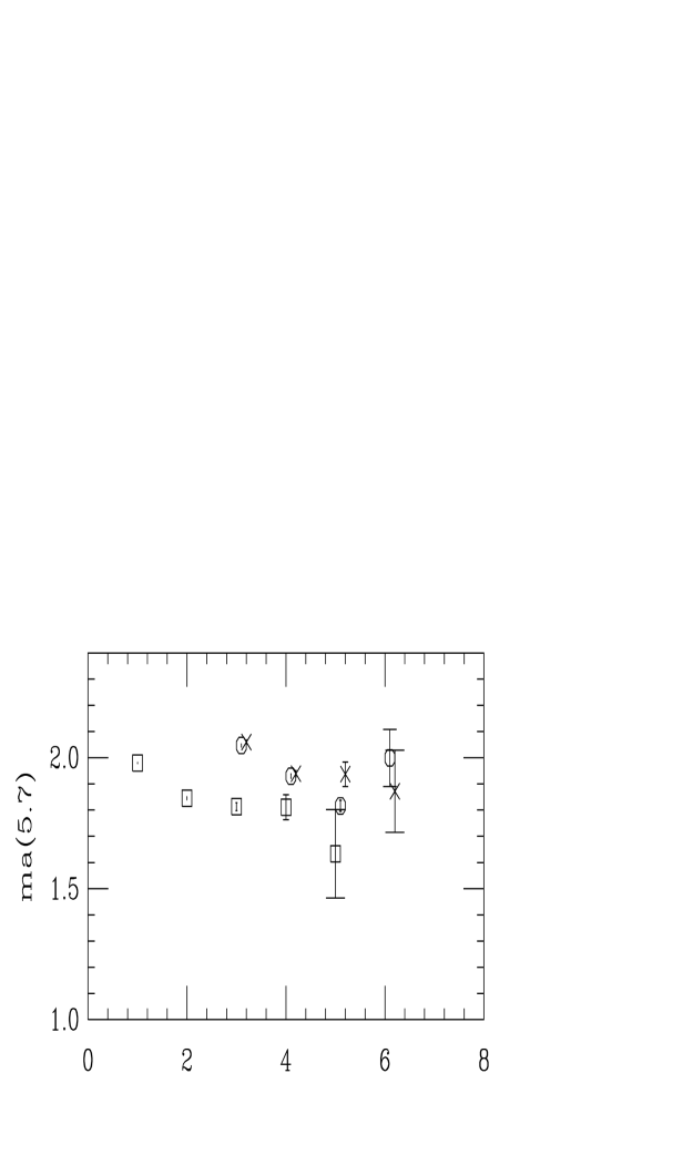
Figure 5: Effective lattice mass versus lattice time for the $V_{A}$ (octagon) and $P_{A}$ (cross) adjoint mesons and $T_{1}^{+-}$ gluelump (square) for $\beta=5.7$ (top) and $\beta=6.0$ (bottom) with light quarks approximately corresponding to strange.

Figure 6: Effective lattice mass versus lattice time for $V_{A}$ at $\beta=6.0$ with two state fit to LL(octagon), LF (cross), and FF (diamond) correlations. Here the light quarks approximately correspond to strange.

The effective masses are plotted in Figure 5. These masses are generated from the optimum combination of paths found in the variational analysis and are plotted as a function of lattice time. We see that at $\beta=5.7$, a plateau is attained indicating that excited state mass contributions are removed. Furthermore the values from the fits to the correlations are in agreement with this plateau value, as shown in Table 6. There is more excited state contamination in the $\beta=6.0$ measurements as shown by the slower approach to a plateau. This is related to the physical time extent of the correlation which is considerably shorter for a given lattice time in the $\beta=6.0$ case (a factor of approximately 1.8). Fitting two states to the matrix of observables for a range $t$-values will be a safer way to extract the ground state mass in this case. This is seen in Table 6 to give a lower mass value than the variational method which strictly gives an upper limit. For the pseudoscalar case at $\beta=6.0$ the signal is considerably more noisy so the plateau assignment is even less clear.

At each $\beta$ value the vector and pseudoscalar adjoint meson masses are very similar. As an estimate of the mass difference, we combine the variational and fit values for strange light quarks at $\beta=5.7$ which yields $M(P_{A})-M(V_{A})=50(70)$ MeV. This result is consistent with the expected situation, as discussed later, that the pseudoscalar meson is slightly heavier than the vector. Since the vector adjoint meson mass is better determined, we base most of our subsequent conclusions on it.

Figure 7: Dependence of the $P_{A}$ (crosses) and $V_{A}$ (squares) masses in units of $r_{0}$ on the light quark mass (evaluated as $r_{0}^{2}M_{\pi}^{2}$) at $\beta=5.7$, showing the extrapolation to the chiral limit.

Figure 8: The mass difference in units of $r_{0}$ between the vector adjoint meson and the lightest gluelump state versus lattice spacing squared ($r_{0}^{-2}(a)\sim a^{2}$). The dotted horizontal line is the experimental pion mass (0.35 in units of $r_{0}$). The adjoint meson results have approximately the same light quark mass (strange).

We now consider finite lattice volume effects. At $\beta=5.7$ we have two lattice volumes available for direct comparisons. We see no significant discrepancies between the adjoint meson masses on these lattices. The spatial volume used at $\beta=6.0$ is comparable to the larger volume at $\beta=5.7$, so should be safe. Of course, in the limit as the light quark mass becomes chiral, these spatial volumes might be inadequate.

The $\kappa$-values used in the calculation corresponded to rather heavy quarks (strange quark or heavier). The adjoint meson, which we model, is composed of $u$ and $d$ quarks. At $\beta=5.7$ we used two values of the quark mass. This enables us to make an extrapolation to light quarks as illustrated in Figure 7. We plot the data from the fits above as $Mr_{0}$ against $(M_{\pi}r_{0})^{2}$ where we expect both quantities to be approximately linear in the constituent quark mass. Thus the figure enables us to make a linear extrapolation in the light quark mass with the chiral limit being the point at which $(M_{\pi}r_{0})^{2}=0$. We find masses in lattice units at the chiral limit of light quarks of $M$=1.808(91) for $V_{A}$ and 1.841(139) for $P_{A}$. Note that this extrapolation corresponds to a difference in mass between a vector adjoint meson with chiral light quarks and one made of $s$-quarks of 73(55)MeV.

The slope of $Mr_{0}$ versus $(M_{\pi}r_{0})^{2}$ that we find at $\beta=5.7$ is consistent, within the large statistical errors, with that found [8] in similar studies of the B-meson and $\Lambda_{b}$ baryon using static $b$-quarks. As noted there, quenched lattice studies tend to find a smaller mass difference than experiment. The experimental value of the $B_{s}$ to $B_{d}$ mass difference is 96 MeV and we might expect the difference of chiral and $s$-quark adjoint mesons to be twice this, which is a smaller value than that we found above. Thus we may conclude that the estimate of the chiral limit of the adjoint mesons quoted above may well have some systematic error, coming either from the extrapolation or from the quenched approximation.

We now consider finite lattice spacing effects and the continuum limit. Since the self energy is unphysical, we study differences between the lightest gluelump and the adjoint meson masses at the same $\beta$ and for a light quark mass corresponding to $s$ quarks. Thus the self energy of the adjoint source is cancelled and we can extract a continuum limit of this splitting. The adjoint meson results use an improved SW-clover action to reduce order $a$ effects. In practice we have used a tadpole improved ansatz for $C_{\rm SW}$ at $\beta=5.7$ which will not completely remove order $a$ effects while the $\beta=6.0$ measurement uses a non-perturbative improvement coefficient, $C_{\rm SW}$, which should remove O(a) effects completely. We plot the mass differences versus $a^{2}$ in Figure 8. This figure shows that the errors are sufficiently large that extrapolation to the continuum limit is not feasible. However, the consistency of the result at our two lattice spacings does suggest that they may be good estimates of the continuum value. Combining the two values then implies a difference $M_{s}(V_{A})-G(1^{+-})$=120(70) MeV.

At $\beta=5.7$, where we are able to make a chiral extrapolation, we find that the $V_{A}$ and $P_{A}$ adjoint mesons are -10(103) MeV and 34(161) MeV, respectively, heavier than the lightest ($1^{+-}$) gluelump. Our result at $\beta=6.0$, though only at one light quark mass, suggests that these mass differences may be somewhat larger. Indeed, combining the values from 5.7 and 6.0 for the $V_{A}$ with $s$ quarks (as above with $M_{s}(V_{A})-G(1^{+-})=120(70)$ MeV) with that for the difference between $s$ quarks and the chiral limit (see above: $M_{s}(V_{A})-M(V_{A})=73(55)$ MeV) yields an overall estimate of the mass difference in the chiral limit of $M(V_{A})-G(1^{+-})=47(90)$ MeV.

4 Discussion

We have made a first non-perturbative study, albeit in the quenched approximation, of the adjoint meson spectrum. We are also able to compare our results for the adjoint meson and the gluelump, since the unphysical lattice self-energy cancels in this comparison. We first summarise some of the phenomenological predictions for these spectra.

In one of the first analyses of this state [1], Chanowitz and Sharpe present a bag model calculation of the adjoint-meson mass spectra, over a range of $M_{\rm gluino}$. They find that the $J^{PC}$ ordering of the vector and pseudoscalar states places the vector particle as being the lighter of the states examined over the range of $M_{\rm gluino}$ examined. Their determination of the spectrum places the lightest gluelump (glueballino) as slightly heavier than the adjoint-meson for larger $M_{\rm gluino}$. Bag model calculations also give the $J^{PC}=1^{+-}$ gluelump as the ground state - the ‘magnetic’ gluon mode.

The ordering of the conventional meson spectrum can be understood qualitatively from the colour-spin interaction arising from one gluon exchange [22]. This interaction makes the pseudoscalar meson lighter than the vector. Now for adjoint mesons, this same one gluon exchange will have a coefficient $-1/8$ of the conventional meson case. This suggests that the level ordering should be reversed - with the vector adjoint meson being lighter. However, the splitting would be much reduced - by a factor of eight. For our light quark masses, the $\pi$ - $\rho$ splitting is anyway smaller than experiment, so we expect near degeneracy of the $V_{A}$ and $P_{A}$ states - as indeed is consistent with our results.

For the flavour non-singlet adjoint meson states, there will be extra terms in the correlation which we have not evaluated. Also there will be mixing with gluelumps states - especially for the vector adjoint meson which mixes with the relatively low-lying $1^{--}$ gluelump.

If the gluino turns out to be the lightest supersymmetric particle and it is stable, it is of interest to establish the set of hadronic bound states of the gluino which are stable. We can make a start on this study by comparing the glueball and adjoint meson spectra we have determined in the quenched approximation. The lightest gluelump has the gluonic field with $J^{PC}=1^{+-}$. The next gluelump state is 368(7) MeV heavier with $J^{PC}=1^{--}$ and, if unmixed, will not be able to decay hadronically to the ground state since both $\pi$ and $2\pi$ modes are forbidden (by isospin and parity respectively). The lightest non-singlet adjoint mesons are the $V_{A}$ and $P_{A}$ and we find them to be somewhat heavier than the lightest gluelump state $G(1^{+-})$, although with a significant systematic error coming from the extrapolation to light quark masses. We obtain $M(V_{A})-G(1^{+-})=47(90)$ MeV. For an adjoint meson composed of $s$ quarks, we have smaller errors since we do not need to make a chiral extrapolation: $M_{s}(V_{A})-G(1^{+-})=120(70)$ MeV and $M_{s}(P_{A})-M_{s}(V_{A})=50(70)$ MeV.

The S-wave hadronic processes $V_{A}\to G(1^{+-})+\pi$ and $G(1^{+-})\to V_{A}+\pi$ are allowed when the $V_{A}$ is composed of $u,\ d$ light quarks. It is thus of interest to establish if the mass difference is such as to make either of these processes an energetically allowed decay. We are unable to answer this categorically because of systematic errors from the various extrapolations needed. However, our results do suggest that the $V_{A}$ is indeed heavier than the $G(1^{+-})$ but that the energy difference is less than $m_{\pi}$, so that $V_{A}$ would be stable. For the $P_{A}$ state, no one pion decay to $G(1^{+-})$ is allowed. An allowed process is $P_{A}\to V_{A}+\pi$ so $P_{A}$ would be unstable if it is more than 140 MeV heavier than $V_{A}$ which does not seem to be the case from our results. As mentioned above, the flavour singlet adjoint mesons are even more difficult to study directly. Mixing with gluelump states may have a significant effect for them and could depress the $1^{--}$ gluelump mass, for instance.

5 Acknowledgements

We thank Janne Peisa for help in developing codes used for stochastic fermions with maximal variance reduction. We acknowledge the support from PPARC under grants GR/L22744 and GR/L55056 and from the HPCI grant GR/K41663, also support from HEFCE via JREI for the SGI Octane at Liverpool.

References

- [1] M. Chanowitz and S. Sharpe, Phys. Lett. 126B, 225 (1983).
- [2] G. R. Farrar and P. Fayed, Phys. Lett, 76B, 575 (1978).
- [3] G. Farrar, Phys. Rev. Lett. 53, 1029 (1984); F. Bucella et al., Phys. Lett. B153, 311 (1985).
- [4] D. Chung et al., Phys. Rev. D57, 4606 (1998).
- [5] I. Jorysz and C. Michael, Nucl. Phys. B302, 448 (1988).
- [6] N. Campbell, I. Jorysz and C. Michael, Phys. Lett. 167B, 91 (1986).
- [7] M. Foster and C. Michael, Nucl. Phys. B (Proc. Suppl.) 63A-C, 724 (1998).
- [8] C. Michael and J. Peisa, Phys. Rev D (in press), hep-lat/9802015.
- [9] C. Michael, Nucl. Phys. (Proc. Suppl.) B6, 417 (1992).
- [10] C. Michael, Acta Phys. Polon. B21, 119 (1990).
- [11] C. Michael, Nucl. Phys. B259, 58 (1985).
- [12] G. Parisi et al., Phys. Lett. 128B, 418 (1983).
- [13] Alpha Collaboration, M. Guagnelli, R. Sommer and H. Wittig hep-lat/9806005.
- [14] R. G. Edwards, U. M. Heller and T. R. Klassen, hep-lat/9711003.
- [15] L.A. Griffiths, C. Michael and P.E.L. Rakow, Phys. Lett. 129B, 351 (1983).
- [16] S. J.Perantonis and C. Michael, Nucl. Phys. B347, 854 (1990).
- [17] K. Juge , J. Kuti and C. Morningstar, Nucl. Phys. B (Proc. Suppl.) 63, 326 (1998); Hadron Spectroscopy, Seventh International Conference, AIP New York 1998, ed. Chung and Willutzki, 137, hep-ph/9711451; contribution to Confinement III, hep-lat/9809015; contribution to LAT98, hep-lat/9809098.
- [18] A. M. Green, C. Michael and P. S. Spencer, Phys. Rev. D55, 1216 (1997).
- [19] C. Michael, Proc. Confinement III, TJ Lab 1998, hep-ph/9809211.
- [20] UKQCD Collaboration, H. P. Shanahan et al., Phys. Rev. D55, 1558 (1997)
- [21] UKQCD Collaboration, R. Kenway, Nucl. Phys. B (Proc. Suppl) 60A, 26 (1998); P. Rowland (private communication).
- [22] A. De Rujula, H. Georgi, and S. Glashow, Phys. Rev. D12, 147 (1975).