CERN-TH/98-350

NORDITA-98/66HE

hep-lat/9811004

THE PHASE DIAGRAM OF THREE-DIMENSIONAL
SU(3)+ADJOINT HIGGS THEORY

K. Kajantie^a,, M. Laine^a,b,, A. Rajantie^c,, K. Rummukainen^d, and M. Tsypin^e,

^aDepartment of Physics, P.O.Box 9, 00014 University of Helsinki, Finland
^bTheory Division, CERN, CH-1211 Geneva 23, Switzerland
^cSchool of CPES, Univ. of Sussex, Brighton BN1 9QJ, UK
^dNORDITA, Blegdamsvej 17, DK-2100 Copenhagen Ø, Denmark
^eDepartment of Theoretical Physics, Lebedev Physical Institute,
Leninsky Prospect 53, 117924 Moscow, Russia

Abstract

We study the phase diagram of the three-dimensional SU(3)+adjoint Higgs theory with lattice Monte Carlo simulations. A critical line consisting of a first order line, a tricritical point and a second order line, divides the phase diagram into two parts distinguished by $\langle{\rm Tr\,}A_{0}^{3}\rangle=0$ and $\not=0$. The location and the type of the critical line are determined by measuring the condensates $\langle{\rm Tr\,}A_{0}^{2}\rangle$ and $\langle{\rm Tr\,}A_{0}^{3}\rangle$, and the masses of scalar and vector excitations. Although in principle there can be different types of broken phases, corresponding perturbatively to unbroken SU(2)$\times$U(1) or U(1)$\times$U(1) symmetries, we find that dynamically only the broken phase with SU(2)$\times$U(1)-like properties is realized. The relation of the phase diagram to 4d finite temperature QCD is discussed.

CERN-TH/98-350
NORDITA-98/66HE
November 1998

1 Introduction

The motivation for studying the three-dimensional (3d) SU(3) + adjoint Higgs gauge theory is twofold. First of all, this case is interesting since the 3d SU(3) + adjoint Higgs theory is an effective theory of finite temperature QCD in the weak coupling domain [1]. The requirement of small couplings means that this effective theory is accurate only in the limit $T\gg\Lambda_{\overline{\rm MS}}$, not in the phase transition region $T\approx T_{c}$ [2]–[5]. For pure gauge SU(3) theory, this is related to the fact that the phase transition at $T=T_{c}$ has to do with the breaking of the Z(3) symmetry. This symmetry is lost in the effective theory, but some traces of it remain, as will be discussed below.

The second interesting aspect of the 3d SU(3) theory is that it already has several of the properties of the SU(5) case, which is relevant for some GUTs at finite temperatures [6]. These properties are not shared by the special SU(2) case, where the structure constants $d_{abc}$ vanish. Such properties are the existence, in perturbation theory, of different types of broken phases with the associated various gauge groups, and of the corresponding monopoles. However, the spectrum of various broken phases is of course richer in SU(5) than in SU(3), and the SU(5) action has also two non-trivial scalar self-couplings in contrast to the SU(3) action, which only has one. Nevertheless, we expect a similar qualitative behaviour.

Some conjectures concerning the phase diagram of the 3d SU(3) + adjoint Higgs theory were put forward in [7]. The purpose of this paper is to determine the phase diagram numerically.

The actions of 3d SU($N\leq 3$) + Higgs theories normally depend on two variables: the scalar mass $m_{3}^{2}$ and the scalar self-coupling $\lambda_{3}$. On the mean field level the system has two phases: a “symmetric” phase at $m_{3}^{2}>0$ and a “broken” phase at $m_{3}^{2}<0$ at any $\lambda_{3}$. The problem now is to determine the phase diagram in the full quantum theory. This question has previously been answered with numerical lattice Monte Carlo simulations for a number of theories: SU(2) + fundamental representation Higgs [8]–[11], SU(2)$\times$U(1) + fundamental Higgs [12], and SU(2) + adjoint Higgs [13, 4]. The case of U(1) + fundamental scalar Higgs (the Ginzburg-Landau theory) has also been extensively studied [14].

For small Higgs self-coupling, $\lambda_{3}\ll g_{3}^{2}$, the tree-level second order transition is, in all cases studied, radiatively changed into a first order transition. Its strength decreases with increasing $\lambda_{3}$. The central and often very difficult question is what happens at larger $\lambda_{3}$: does the first order line terminate (so that the two phases are analytically connected) or is there a phase transition line across the whole phase diagram (so that there is an order parameter vanishing in one of the phases). In this respect, the phase diagrams for the different symmetry groups differ in quite interesting ways from each other. A good illustration of the difficulty of the problem is the fact that the nature of the phase diagram in the superficially simplest case, the Ginzburg-Landau theory, is not yet conclusively determined in the large $\lambda_{3}$, extreme type II, regime.

For SU(3) + adjoint Higgs theory we shall see that the phase diagram is divided into two parts by a phase transition line which contains a first order line, a tricritical point and a second order line. In contrast, the SU(2) + adjoint Higgs theory is observed to have no transition at large $\lambda_{3}$ [13]. The reason why it is possible to have a qualitatively different behaviour in SU(2) and SU(3) is that for all SU($N\geq 3$) there is a gauge-invariant local order parameter $\langle{\rm Tr\,}A_{0}^{3}\rangle$ sensitive to the breaking of the $A_{0}\leftrightarrow-A_{0}$ symmetry of the theory.

The plan of the paper is the following. In Sec. 2 we define the theory in continuum and on the lattice. In Sec. 3 we present some perturbative estimates for the different observables measured, and in Sec. 4 we briefly review the relation to 4d finite temperature QCD. The simulation results are in Sec. 5, and the conclusions in Sec. 6.

2 Definition of SU(3) + adjoint Higgs theory

The theory we study is defined by the following super-renormalizable Lagrangian:

$$L[A_{i}^{a},A_{0}^{a}] = {\frac{1}{4}}F_{ij}^{a}F_{ij}^{a}+{\rm Tr\,}[D_{i},A_{0}][D_{i},A_{0}]+m_{3}^{2}{\rm Tr\,}A_{0}^{2}+\lambda_{A}({\rm Tr\,}A_{0}^{2})^{2},$$ (1)

in standard notation ($D_{i}=\partial_{i}+ig_{3}A_{i}$). The notation $A_{0}=A_{0}^{a}T^{a}$ for the adjoint scalar is chosen with its origin from dimensional reduction of QCD in mind. For SU(3) and SU(2) ${\rm Tr\,}A_{0}^{4}={\frac{1}{2}}({\rm Tr\,}A_{0}^{2})^{2}$ so that only one scalar self-coupling appears. In principle, there could also be two additional super-renormalizable couplings $h_{3},h_{5}$ appearing as

$$\delta L=h_{3}{\rm Tr\,}A_{0}^{3}+h_{5}{\rm Tr\,}A_{0}^{2}{\rm Tr\,}A_{0}^{3}.$$ (2)

However, these terms do not arise in the dimensional reduction of finite temperature QCD, and thus we assume that $h_{3}=h_{5}=0$.

In the absence of $h_{3},h_{5}$, the theory in Eq. (1) is symmetric under $A_{0}\to-A_{0}$. This symmetry was called “R-parity” in [7]. In terms of 4d physics, this symmetry is related to the usual discrete transformations CT, P [15, 16]. However, it should be clearly stated that the breaking of the $A_{0}\to-A_{0}$ symmetry to be discussed below, does certainly not imply spontaneous breaking of any of the discrete symmetries of finite temperature QCD, since the broken phases are not physical from the point of view of QCD [4].

Due to super-renormalizability, of the couplings in Eq. (1) only the scalar mass $m_{3}^{2}$ is scale dependent. In the $\overline{\mbox{\rm MS}}$ scheme

$$m_{3}^{2}(\mu)={f_{2}\over 16\pi^{2}}\ln{\Lambda\over\mu},\quad f_{2}=20(3g_{3}^{2}-\lambda_{A})\lambda_{A},$$ (3)

where $\Lambda$ is a constant of dimension GeV. The dynamics of the theory is thus determined by the dimensionless variables

$$y={m_{3}^{2}(g_{3}^{2})\over g_{3}^{4}},\quad x={\lambda_{A}\over g_{3}^{2}},$$ (4)

where $g_{3}^{2}$ has been used as a natural mass unit.

Instead of regulating the theory using the $\overline{\mbox{\rm MS}}$ scheme one can as well use the lattice scheme with a lattice constant $a$. The two schemes have to be matched so that they, in the limit $a\to 0$ and for given $g_{3}^{2},y,x$, give the same physical results. Due to the super-renormalizability this only requires tuning the bare mass term of the lattice action. Introducing the gauge coupling constant $\beta_{G}$ by

$$\beta_{G}={6\over ag_{3}^{2}},$$ (5)

the lattice action $S=S[U_{i}({\bf x}),A_{0}({\bf x})]$ becomes

$$S = \beta_{G}\sum_{\bf x}\sum_{i<j}(1-{\frac{1}{3}}{\rm Re}{\rm Tr\,}P_{ij}({\bf x}))$$ (6)

$$-{12\over\beta_{G}}\sum_{{\bf x},i}{\rm Tr\,}A_{0}({\bf x})U_{i}({\bf x})A_{0}({\bf x}+i)U_{i}^{\dagger}({\bf x})$$

$$+\sum_{i}\left\{\beta_{2}{\rm Tr\,}A_{0}^{2}({\bf x})+x{216\over\beta_{G}^{3}}[{\rm Tr\,}A_{0}^{2}({\bf x})]^{2}\right\},$$

where $P_{ij}({\bf x})$ is the plaquette and where the coefficient of the quadratic term is [17]

$$\beta_{2} = {36\over\beta_{G}}\left\{1+{6\over\beta_{G}^{2}}y-(6+10x){3.1759115\over 4\pi\beta_{G}}\right.$$ (7)

$$\left.-{6\over 16\pi^{2}\beta_{G}^{2}}[(60x-20x^{2})(\ln\beta_{G}+0.08849)+34.768x+36.130]\right\}.$$

Remarkably, the matching of lattice and continuum can be carried out analytically even including terms of order $a$ [18]. This implies that the $g_{3}^{2},y,x$ in Eq. (6) are modified by corrections of order $1/\beta_{G}$. The additive corrections for $y$ have not yet been computed: the ${\cal O}(a)$ correction is, for dimensional reasons, $\sim ag_{3}^{6}f(x,y)$ and a 3-loop computation would be needed. For the two other parameters the improvements are

$$(g_{3}^{2})_{\mbox{\scriptsize improved}} = \left(1+{1.994833\over\beta_{G}}\right)g_{3}^{2},$$

$$x_{\mbox{\scriptsize improved}} = x-{1\over\beta_{G}}(0.328432-0.835282x+1.167759x^{2}),$$ (8)

where $g_{3}^{2},x$ are the parameters appearing in Eqs. (5)–(7).

The improved relations between the condensates of the scalar field $A_{0}$ in the lattice action in Eq. (6) and in the continuum are

$${\langle{\rm Tr\,}A_{0}^{2}\rangle_{\mbox{\scriptsize cont}}\over g_{3}^{2}} = \bigg{(}\langle{\rm Tr\,}A_{0}^{2}\rangle-{3.1759115\beta_{G}\over 6\pi}\bigg{)}\bigg{(}1-{\frac{3.409891-0.729850x}{\beta_{G}}}\bigg{)}$$ (9)

$$-{3\over 2\pi^{2}}(\ln\beta_{G}+0.6678),$$

$${\langle{\rm Tr\,}A_{0}^{3}\rangle_{\mbox{\scriptsize cont}}\over g_{3}^{3}} = \langle{\rm Tr\,}A_{0}^{3}\rangle\bigg{(}1-{\frac{5.114364-0.437910x}{\beta_{G}}}\bigg{)}.$$ (10)

In Eq. (9) an ${\cal O}(ag_{3}^{2})$ additive 3-loop correction is still not known. The $1/\beta_{G}$-terms are numerically quite large at the value $\beta_{G}=12$ we have used in practice (up to $\sim 40\%$), and implementing them brings the lattice results significantly closer to the perturbative results (deep in the perturbative regime).

The $\overline{\mbox{\rm MS}}$-scheme regularized operator $\langle{\rm Tr\,}A_{0}^{2}\rangle_{\mbox{\scriptsize cont}}$ is, in fact, scale dependent [19], and has been defined at the scale $\mu=g_{3}^{2}$ in Eq. (9). The scale dependence arises at the 2-loop level and is, for general $N$,

$$\langle{\rm Tr}A_{0}^{2}\rangle(\mu^{\prime})=\langle{\rm Tr}A_{0}^{2}\rangle(\mu)+{g_{3}^{2}(N^{2}-1)N\over 16\pi^{2}}\ln{\mu^{\prime}\over\mu}.$$ (11)

In terms of the effective potential (note that $\langle{\rm Tr\,}A_{0}^{2}\rangle_{\mbox{\scriptsize cont}}=dV(\mbox{min})/dm_{3}^{2}$), the scale dependence arises from the graph (solid line = $A_{0}$, wavy line = $A_{i}$)

$$\parbox[c]{42.67912pt}{ \begin{picture}(30.0,30.0)(0.0,0.0) \put(0.0,0.0){} \put(0.0,0.0){} \end{picture}}\propto{g_{3}^{2}(N^{2}-1)N\over 16\pi^{2}}m_{3}^{2}\biggl{(}\ln{\mu\over 2m_{3}}+{\frac{3}{4}}\biggr{)}.$$ (12)

It is amusing to note that this term is precisely the ${\cal O}(g^{4}\ln(g))$ Toimela term [20, 3] in the free energy of the QCD plasma.

The gauge invariant operators of lowest dimensionalities in the action defined by Eq. (6) are as follows:

• Dim=1: ${\rm Tr\,}A_{0}^{2}$,

• Dim=3/2: ${\rm Tr\,}A_{0}^{3}$,

• Dim=2: $({\rm Tr\,}A_{0}^{2})^{2}$, $\epsilon_{ijk}{\rm Tr\,}A_{0}F_{jk}$,

• Dim=5/2: $\epsilon_{ijk}{\rm Tr\,}A_{0}^{2}F_{jk}$,

• Dim=3: ${\rm Tr\,}F_{ij}F_{kl}$, ${\rm Tr\,}[D_{i},A_{0}]\,[D_{j},A_{0}]$ (with various spin projections).

These operators can be used for mass measurements in the different quantum number channels.

3 Perturbation theory

Because of confinement, perturbation theory is not well convergent in the symmetric phase of the theory and is thus, in general, of limited usefulness in the study of the phase structure. Nevertheless, perturbation theory does work in the limit of small $x=\lambda_{A}/g_{3}^{2}$ when the transition becomes very strong, and it is worthwhile to go through its predictions there.

Let us first fix a gauge and parametrise a constant diagonal SU(3) background field as follows:

$$g_{3}^{-1}\langle A_{0}\rangle=B=B_{3}T^{3}+B_{8}T^{8}=\left(\begin{array}[]{ccc}q+p&0&0\\ 0&q-p&0\\ 0&0&-2q\end{array}\right),$$ (13)

with

$${\rm Tr\,}B^{2}=6q^{2}+2p^{2},\quad{\rm Tr\,}B^{3}=6q(p^{2}-q^{2}),\quad{\rm Tr\,}B^{4}={\frac{1}{2}}({\rm Tr\,}B^{2})^{2}.$$ (14)

(Note that ${\rm Tr\,}B^{2}=g_{3}^{-2}{\rm Tr\,}\langle A_{0}\rangle^{2}\neq g_{3}^{-2}\langle{\rm Tr\,}A_{0}^{2}\rangle.$) If $p=0$ or $p=\pm 3q$, then the SU(3) symmetry is broken to SU(2)$\times$U(1), otherwise it is broken to U(1)$\times$U(1). These are perturbative statements; the only symmetry that can be broken in the full quantum theory is $A_{0}\leftrightarrow-A_{0}$, which is signalled by $\langle{\rm Tr\,}A_{0}^{3}\rangle$.

3.1 The $x\to 0$ limit

Let us compute the 1-loop effective potential $V_{1}(x,y;q,p)$ in the background in Eq. (13). One finds, in the Landau gauge,

$$g_{3}^{-6}V(x,y;q,p)=y(6q^{2}+2p^{2})+x(6q^{2}+2p^{2})^{2}$$

$$-{1\over 3\pi}(|3q+p|^{3}+|3q-p|^{3}+8|p|^{3})$$

$$-{1\over 12\pi}\left\{[y+6x(6q^{2}+2p^{2})]^{3/2}+7[y+2x(6q^{2}+2p^{2})]^{3/2}\right\}.$$ (15)

The scalar loop terms (last line in Eq. (15)) become negligible when $x\to 0$ (apart from a constant) and we shall neglect them to begin with. Then, for $p=0$,

$$g_{3}^{-6}V(x,y;q,0)=36xq^{2}\left[\left(|q|-{1\over 4\pi x}\right)^{2}+{1\over 6x}\left(y-{3\over 8\pi^{2}x}\right)\right].$$ (16)

Thus, for

$$y=y_{c}^{\mbox{\scriptsize 1loop}}(x)={3\over 8\pi^{2}x}$$ (17)

the system has two coexisting states (a first order transition) with

$$q_{\mbox{\scriptsize symmetric}}=0,\qquad q_{\mbox{\scriptsize broken}}={1\over 4\pi x}.$$ (18)

One stable and one metastable state exists for

$$y_{-}(x)=0<y<y_{+}(x)={9\over 8}y_{c}(x).$$ (19)

These results for $p=0$ can now be extended to the whole $(q,p)$-plane. Indeed,

$$V_{1}(x,y;q>0,p=3q)=V_{1}(x,y;2q,0),\quad V_{1}(x,y;q<0,p=-3q)=V(x,y;2q,0).$$ (20)

This implies that, at $y=y_{c}(x)$, the system has the following degenerate potential minima (Fig.1):

• a symmetric minimum at $q=0$, $p=0$,

• a broken minimum at $q=1/(8\pi x),\,\,p=3/(8\pi x)$,

• a broken minimum at $q=1/(4\pi x)$, $p=0$.

Moreover, in the parametrisation in Eq. (13) one has the freedom of permuting the diagonal elements and the potential has to be invariant under the transformations of $q,p$ corresponding to these permutations. One sees that the fundamental region, which determines the potential over the whole plane, can be chosen to be that bounded by the two lines $p=0,\,p=3q$. Thus, for each broken minimum there are two more minima corresponding to cyclic permutations of the diagonal elements. All these minima correspond to breaking to SU(2)$\times$U(1); there are no local minima corresponding to breaking to U(1)$\times$U(1) (a U(1)$\times$U(1) minimum would require that all the vector masses cubed appearing on the 2nd line in Eq. (15) are non-vanishing, but this is not the case in any of the minima considered).

   

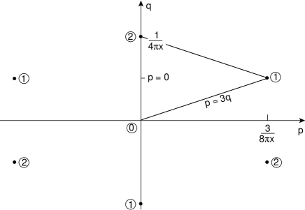
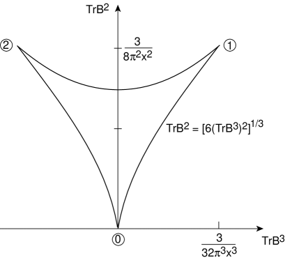
Figure 1: The minima of the 1-vectorloop potential on the critical line $y=y_{c}(x)$ (Eq. (17)). Left: The minima in the $(q,p)$-plane. Those with the same number correspond to permutations of the eigenvalues of $B$ in Eq. (13). The fundamental region is bounded by the two lines $p=0,\,p=3q$. Right: The minima in the $({\rm Tr\,}B^{2},{\rm Tr\,}B^{3})$-plane. The boundary curve is the map of the triangle in the left panel.

To get rid of the unphysical extra symmetries related to the permutation of the diagonal elements of $B$ in Eq. (13), it is useful to write the 1-loop potential in terms of ${\rm Tr\,}B^{2}$ and ${\rm Tr\,}B^{3}$. Effectively, one inverts the cubic Eqs. (14) and inserts into Eq. (15). The result is

$$V_{1}(x,y;{\rm Tr\,}B^{2},{\rm Tr\,}B^{3})=y{\rm Tr\,}B^{2}+x({\rm Tr\,}B^{2})^{2}$$

$$-{1\over 3\pi}\left\{{\rm Tr\,}B^{2}{\rm Re}\left[\left({\frac{9}{2}}{\rm Tr\,}B^{3}+{\frac{3}{2}}\sqrt{3}i\sqrt{{\frac{1}{2}}({\rm Tr\,}B^{2})^{3}-3({\rm Tr\,}B^{3})^{2}}\right)^{1/3}(3-i\sqrt{3})\right]\right.$$

$$-\left.\sqrt{{\frac{1}{2}}({\rm Tr\,}B^{2})^{3}-3({\rm Tr\,}B^{3})^{2}}\right\}\Theta\Bigl{[}{\frac{1}{2}}({\rm Tr\,}B^{2})^{3}-3({\rm Tr\,}B^{3})^{2}\Bigr{]}.$$ (21)

This form, containing the solution of a cubic equation, is not very transparent, but it actually is quite simple, as shown in Fig.1. Now only the genuinely different minima, one symmetric and two broken ones, appear.

Summarising, for $x\to 0$ perturbation theory predicts that the system has the following three phases:

• one symmetric phase with ${\rm Tr\,}B^{2}={\rm Tr\,}B^{3}=0$ for $y>y_{c}^{\mbox{\scriptsize 1loop}}(x)$,

• two broken phases for $y<y_{c}^{\mbox{\scriptsize 1loop}}(x)$, distinguished by the sign of ${\rm Tr\,}B^{3}$.

In the broken phase at the critical point $y=y_{c}$,

$${\rm Tr\,}B^{2} = {3\over 8\pi^{2}x^{2}}\approx 3.80\left({0.1\over x}\right)^{2},$$

$${\rm Tr\,}B^{3} = \pm{3\over 32\pi^{3}x^{3}}\approx\pm 3.02\left({0.1\over x}\right)^{3}.$$ (22)

3.2 Condensates

Using the effective potential in Eq. (15), one can calculate the 1-loop perturbative approximation for $\langle{\rm Tr}A_{0}^{2}\rangle$,

$$g_{3}^{-2}\langle{\rm Tr}A_{0}^{2}\rangle=g_{3}^{-6}{\partial V\over\partial y}=6q^{2}-\frac{1}{8\pi}\left[(y+36xq^{2})^{1/2}+7(y+12xq^{2})^{1/2}\right],$$ (23)

where $q$ is obtained by minimizing the potential in Eq. (15) with $p=0$ and is zero in the symmetric phase. A similar calculation yields

$$g_{3}^{-3}\langle{\rm Tr\,}A_{0}^{3}\rangle=\pm\left\{6q^{3}-\frac{3q}{8\pi}\left[(y+36xq^{2})^{1/2}-(y+12xq^{2})^{1/2}\right]\right\}.$$ (24)

At the limit $x\to 0$ considered in Eq. (22), $g_{3}^{-2}\langle{\rm Tr}A_{0}^{2}\rangle={\rm Tr\,}B^{2}-(y^{1/2}/\pi)$, $g_{3}^{-3}\langle{\rm Tr\,}A_{0}^{3}\rangle={\rm Tr\,}B^{3}$. Note that the perturbative $\overline{\mbox{\rm MS}}$ value of $\langle{\rm Tr}A_{0}^{2}\rangle$ is negative in the symmetric phase.

3.3 What happens at larger $x$?

When $x$ increases, the scalar contributions become more important, perturbation theory becomes less accurate, the three well separated phases in Fig.1 approach each other, and the transition gets weaker. In the case of the SU(2) + adjoint Higgs theory this leads to an endpoint of the first order line [13]: there is no local order parameter, and the phases are believed to be analytically connected. In the present case, the transition also becomes weaker with increasing $x$. However, now there is a gauge invariant local order parameter, $\langle{\rm Tr\,}A_{0}^{3}\rangle$, which can signal the breaking of the Z(2) symmetry $A_{0}\to-A_{0}$ of the theory. Thus we expect that the $(x,y)$-plane phase diagram can be disconnected by a critical line containing a first order transition at $x<x_{c}$, a tricritical point  at $x=x_{c}$, and a second order line at $x>x_{c}$.

However, as is standard in the case of tricritical transitions, in order to see the full phase diagram one has to use three couplings/fields. In our case the couplings are $x$, $y$ and $h$, an external field with a coupling $h{\rm Tr\,}A_{0}^{3}$ (see Eq. (2)). The schematic 3-dimensional phase diagram is shown in the left panel of Fig. 2. We note that in this full coupling space the three phases are still analytically connected through the large $x$ region.

    

Figure 2: Schematic phase diagrams of systems with a tricritical point (left) and a quadruple point (right), shown in a 3-dimensional coupling space $(x,y,h)$, where $h$ is an external field which couples to ${\rm Tr\,}A_{0}^{3}$. The surfaces are 1st order phase transitions, and dashed lines 2nd order (Ising) transitions. The 1st order surfaces join along lines of triple points, where three phases are separated by 1st order phase transitions. At the quadruple point (right) four phases are separated by 1st order transitions; this is an intersection point of four lines of triple points and six surfaces of 1st order transitions.

In principle, more complicated phase structures are also possible. At large enough $x$ a new phase with $\langle{\rm Tr\,}A_{0}^{3}\rangle=0$, $\langle{\rm Tr\,}A_{0}^{2}\rangle>0$ may appear (compare with the symmetry breaking patterns shown in Eq. (14)!). There is no local order parameter separating this phase form the symmetric one, but perturbatively it corresponds to a phase with the gauge group U(1)$\times$U(1). If this occurs, there will be a quadruple point at some value of $x$, where four phases separated by 1st order transitions can exist (see the right panel of Fig. 2). The phase structure suggested in [7] belongs to this class, even though the authors discussed the phases only in the $(x,y)$-plane.

This kind of phase structure with a quadruple point is known to exist in some theories, for example, in the 3d 3-state Potts model [21] and, indeed, in the finite temperature pure SU(3) gauge theory in 3+1 dimensions. These models have an exact Z(3) symmetry, and they have 3 degenerate broken phases and 1 unbroken phase, which can all exist at the quadruple point. For the case of SU(3) gauge theory, the 3d phase diagram is spanned by $1/T$ and external fields coupling to the real and imaginary parts of the Polyakov line. Indeed, the phase space of the Polyakov line in the complex plane does resemble the phase structure of the SU(3) + adjoint Higgs theory, shown in Fig. 1. If one considers the SU(3) + adjoint Higgs theory as a dimensionally reduced version of the 4d gauge theory, it is appealing to think that the phase structures of the two theories could be similar. However, one has to bear in mind that in the 3d adjoint Higgs theory the 3-fold symmetry of the original 4d theory is strongly broken, as will be discussed in the next section. Even then it is not impossible that the Z(3) symmetry is dynamically generated in the close proximity of the would-be tricritical point (this can be compared with the dynamically generated Ising symmetry in the SU(2) gauge + fundamental Higgs theory [11]). If this truly happens, the would-be tricritical point could transform into a quadruple point.

The question about the nature of the phase diagram is settled numerically below, and it will turn out that the phase diagram is the standard tricritical one, as shown in the left part of Fig. 2.

4 Relation to 4d and to Z($N$) symmetry

The relation between $x,y$ and 4d physics ($T,\Lambda_{\overline{\rm MS}},N,N_{f}$) is worked out explicitly to leading + next-to-leading order in [4, 22]. For $N=3,N_{f}=0$ the answer is

$$x = {3\over 8\pi^{2}}g^{2}(4\pi e^{-\gamma_{E}-3/11}T)$$ (25)

$$= {3\over 11}\,\,{1\over\ln(5.371T/\Lambda_{\overline{\rm MS}})},$$

$$y \equiv y_{\mbox{\scriptsize dr}}(x)={3\over 8\pi^{2}x}+{9\over 16\pi^{2}}+{\cal{O}}(x).$$ (26)

As discussed, the 4d finite $T$ theory without matter in the fundamental representation possesses an extra symmetry, the Z($N$) symmetry, for which the thermal Wilson line

$$L({\bf x})={1\over N}{\rm Tr\,}P\exp\left[ig\int_{0}^{\beta}d\tau A_{0}(\tau,{\bf x})\right]$$ (27)

is an order parameter: if $z_{k}=\exp(i2\pi k/N)$ one can define a transformation of the fields so that the action is invariant but $L\to z_{k}L$. Thus $\langle L({\bf x})\rangle$ acts as an order parameter.

This symmetry, however, is lost in the reduction process. The reason is simply that in the reduction process mass scales $\sim\pi T$ are integrated over. However, under a Z($N$) transformation a field configuration with small fields is transformed to one with $A_{0}\sim\pi T/g$ and the reduction process cannot accurately represent such large scales.

Even though the exact symmetry is lost, part of it is restored by radiative effects in the effective theory. The leading order term in Eq. (26) coincides with the leading order critical line Eq. (17). This can be seen as a remnant of the Z($N$) symmetry, since in this approximation, the effect of the Z($N$) transformations of the 4d theory is to move the system from one of the three degenerate minima of Fig. 1 to another. This degeneracy is lost when higher-order corrections are taken into account, and the true transition line of the 3d theory does not agree with the dimensional reduction line. Moreover, in the effective 3d theory, only the vertices marked by 1 and 2 are related by the symmetry of the theory; in hot QCD (and in the 3d 3-state Potts model) all the vertices are equivalent. It is thus also natural that in the effective theory the middle point of the triangular region in Fig. 1 plays no special role, in contrast to the situation in hot QCD, where the middle point corresponds to the confined phase.

5 Simulation results

The primary aim of the simulations is to resolve the nature of the phase diagram and find the $(x,y)$-plane critical curve $y=y_{c}(x)$. We also measure the screening masses (inverse screening lengths) on both sides of the transition line at various values of $x$.

$x$	Volumes
0.10	$12^{3}$
0.15	$16^{3}$
0.20	$16^{3}$,  $32^{3}$
0.25	$16^{3}$,  $24^{3}$,  $32^{3}$,  $48^{3}$
0.30	$16^{3}$,  $32^{3}$

Table 1: The lattice sizes used at $\beta_{G}=12$. For $0.15\leq x\leq 0.30$ several values of $y$ were used for each $x$, both above and below the transition. For $x\leq 0.20$, multicanonical simulations were used at $y=y_{c}(x)$.

The simulations were performed using $\beta_{G}=6/(g_{3}^{2}a)=12$, with $x$ in the interval $0.10\leq x\leq 0.30$. The use of only one lattice spacing (one $\beta_{G}$) precludes the extrapolation of the results to the continuum limit. However, we expect the finite lattice spacing effects to be small enough for the purpose of mapping the phase diagram. This is supported by our experiences from the measurement of the phase diagram of the SU(2) + adjoint Higgs model [4].

The lattice volumes and the values of $x$ used in this study are listed in Table 1. For each $x$ and lattice size, several runs at various values of $y$ were performed. The total number of runs was 72, with approximately 2.1 node-years of cpu-time on a Cray T3E. This corresponds to $\sim 2\times 10^{16}$ floating point operations at 130 Mflops/node.

5.1 Local order parameters

For $x\leq 0.2$, the transition point $y=y_{c}(x)$ was determined with multicanonical simulations using only lattices of size $12^{3}$ and $16^{3}$. The transition here is so strongly of the first order – that is, the latent heat and the surface tension are so large – that the system tunnels from one phase to another too infrequently, even when multicanonical simulations are used. The value of $y_{c}(x)$ was determined to be the value of $y$ where the probability weight of each of the 3 phases is equal.

   $x=0.15$ $x=0.20$

$x=0.25$

Figure 3: The probability distributions in the $({\rm Tr\,}A_{0}^{3},{\rm Tr\,}A_{0}^{2})$-plane at $y=y_{c}(x)$, $x=0.15$, $0.20$, $0.25$. The data is from $16^{3}$, $\beta_{G}=12$ simulations; the simulations at $x=0.15$ and $x=0.20$ are multicanonical.

The strength of the transition is illustrated in Fig. 3, where we show the probability distribution in the $({\rm Tr\,}A_{0}^{3},{\rm Tr\,}A_{0}^{2})$-plane on the transition line for $x=0.15$…0.25. For small $x$, the three peaks are very strongly separated, but when $x$ approaches 0.25, the peaks join. It should be noted that in each case, the two ${\rm Tr\,}A_{0}^{2}>0$ peaks are always connected by a “tunnelling channel” to the ${\rm Tr\,}A_{0}^{2}\approx 0$ phase. When $x=0.15$, the relative probability density in these channels is suppressed by a factor $\sim 10^{-9}$ when compared with the peaks, making them utterly invisible in Fig. 3, plotted with a linear scale. At $x=0.2$, this suppression is “only” a factor of $\sim 0.01$, and at $x=0.25$, there is no significant suppression any more. Note that the magnitude of the suppression is not universal and it depends very strongly on the volume of the system. Indeed, in large enough volumes the magnitude of the suppression can be related to the interface tension $\sigma$ between the phases. However, the volumes used here are too small for a reliable determination of $\sigma$.

It should be noted that there is no “tunnelling channel” directly connecting the two ${\rm Tr\,}A_{0}^{2}>0$ peaks even near the tricritical point. Thus, the tunnelling from one of these peaks to the other always proceeds through the region of the ${\rm Tr\,}A_{0}^{2}\approx 0$ peak. This indicates that there is no  dynamical generation of the Z(3) symmetry, and the behaviour is the standard tricritical one.

In fact, we did not observe any sign of the quadruple point and the associated new phase in any point of the $(x,y)$-plane (since $\langle{\rm Tr\,}A_{0}^{2}\rangle,\langle{\rm Tr\,}A_{0}^{3}\rangle$ are always simultaneously small or large, see below). This indicates that the phase diagram shown in the right panel of Fig. 2 is not relevant here.

   

   

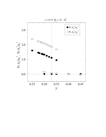
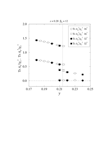
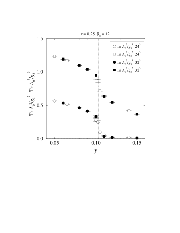
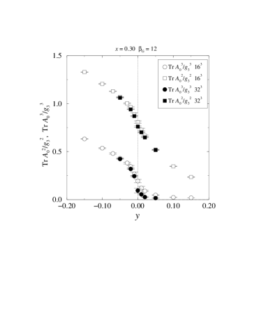
Figure 4: The condensates $\langle{\frac{1}{N^{3}}}\sum_{x}{\rm Tr\,}A_{0}^{2}/g_{3}^{2}\rangle$ and $\langle|{\frac{1}{N^{3}}}\sum_{x}{\rm Tr\,}A_{0}^{3}/g_{3}^{3}|\rangle$ measured across the transition at $x=0.15$, 0.20, 0.25 and 0.30 (converted to continuum units according to Eqs. (9), (10)). The broken phase values compare quite well with the 1-loop perturbative ones in Eqs. (23), (24) for $x=0.15$.

In Fig. 4 we show the behaviour of the dim-1 and dim-(3/2) condensates (scaled by a proper power of $g_{3}$ to make them dimensionless),

$$\langle{\frac{1}{N^{3}}}\sum_{x}{\rm Tr\,}A_{0}^{2}/g_{3}^{2}\rangle~{}~{}~{}~{}~{}\mbox{and}~{}~{}~{}~{}~{}\langle|{\frac{1}{N^{3}}}\sum_{x}{\rm Tr\,}A_{0}^{3}/g_{3}^{3}|\rangle,$$ (28)

at $0.15\leq x\leq 0.30$ across the transition. Note that in the latter case a projection to positive values is needed, since otherwise the operator would always yield zero when measured from a finite volume. In the infinite volume limit, $\langle|{\frac{1}{N^{3}}}\sum_{x}{\rm Tr\,}A_{0}^{3}/g_{3}^{3}|\rangle$ is perturbatively given by Eq. (24). In the figures, the lattice operators in Eq. (28) are converted to continuum units according to Eqs. (9), (10).

   

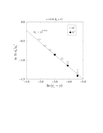
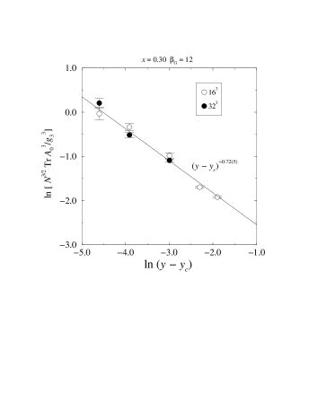
Figure 5: The scaling behaviour of $\langle|{\frac{1}{N^{3}}}\sum_{x}{\rm Tr\,}A_{0}^{3}/g_{3}^{3}|\rangle$ for $y<y_{c}$ (left), $y>y_{c}$ (right), at finite volumes and in a suitable range of $y$. The data is the same as in Fig. 4. The Ising model exponents are $\approx 0.33$ for $y<y_{c}$ and $\approx-0.62$ for $y>y_{c}$ (see, e.g., [23]). The continuous lines are fits to the $32^{3}$ data.

At $x\leq 0.2$ the transition is strongly of the 1st order, and there is a substantial metastability range across the transition point $y_{c}$. However, the operator $\langle|{\frac{1}{N^{3}}}\sum_{x}{\rm Tr\,}A_{0}^{3}/g_{3}^{3}|\rangle$, which has no additive renormalization, remains a good order parameter at all values of $x$, even when the metastability disappears at $x\mathop{\raise 1.29167pt\hbox{$>$\kern-7.5pt\raise-4.73611pt\hbox{$\sim$}}}0.25$. Its deviation from zero at $y>y_{c}$ is a well understood finite volume effect: for large enough volumes, it is proportional to $1/\sqrt{\mbox{volume}}$.

At $x=0.30$ we are substantially away from the first order region, and at $y=y_{c}$ there is a second order transition separating the two $\langle{\rm Tr\,}A_{0}^{3}\rangle\neq 0$ phases from the $\langle{\rm Tr\,}A_{0}^{3}\rangle=0$ phase. Indeed, ${\rm Tr\,}A_{0}^{3}$ behaves exactly as magnetization in the 3d Ising model (this can be understood by comparing the regime $x>x_{\mbox{\scriptsize tricritical}}$ of the phase diagram in the left panel in Fig. 2 with that of the Ising model). We verify the Ising type of the transition by examining the critical behaviour of $\langle|{\frac{1}{N^{3}}}\sum_{x}{\rm Tr\,}A_{0}^{3}/g_{3}^{3}|\rangle$ in the neighbourhood of $y_{c}$. For $y<y_{c}$ and in the infinite volume limit it approaches zero with the critical exponent $\beta\approx 0.33$:

$$\langle|{\frac{1}{N^{3}}}\sum_{x}{\rm Tr\,}A_{0}^{3}/g_{3}^{3}|\rangle\propto(y_{c}-y)^{\beta}.$$ (29)

When $y>y_{c}$, $\langle|{\frac{1}{N^{3}}}\sum_{x}{\rm Tr\,}A_{0}^{3}/g_{3}^{3}|\rangle=0$ in the infinite volume limit. However, at a finite volume, its behaviour can be approximated in some range of $y$ (where the linear extension of the lattice is still much larger than the longest correlation length) as

$$\langle|{\frac{1}{N^{3}}}\sum_{x}{\rm Tr\,}A_{0}^{3}/g_{3}^{3}|\rangle\propto N^{-3/2}(y-y_{c})^{-\gamma/2}\,,$$ (30)

where for the 3d Ising model $\gamma\approx 1.24$. As can be seen from Fig. 5, the data agree rather well with these Ising model expectations.

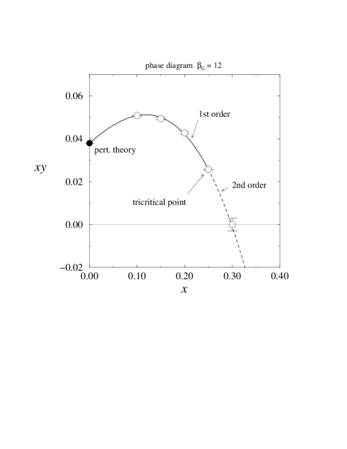
Figure 6: The phase diagram of the 3d SU(3) + adjoint Higgs theory. The open symbols are results from the simulations, and the filled circle is the perturbative result in Eq. (17). The transition line is a polynomial fit to the data.

The measured $(x,y)$-plane phase diagram is shown in Fig. 6. The first order line is converted into a second order transition at a tricritical point, which is approximately located at $x_{c}\approx 0.26$, $y_{c}\approx 0.104$ ($x_{\mbox{\scriptsize{\it c}, improved}}\approx 0.24$ according to Eq. (8)). The fact that there is a second order transition at $x>x_{c}$, is based on the observations that (1) the transition is not of the first order since the local order parameters behave continuously (Fig. 4), (2) there is a real symmetry $A_{0}\to-A_{0}$ which gets broken, and shows the scaling expected (Fig. 5), (3) the correlation length related to $A_{0}$ seems to diverge at the transition point (Sec. 5.2).

The critical exponents associated with the tricritical point in 3d assume their mean field values. We did not attempt to numerically analyze the critical properties at the tricritical point, since a meaningful analysis would have required simulations with much larger volumes and higher statistics than those used in this work.

5.2 Correlation lengths

   

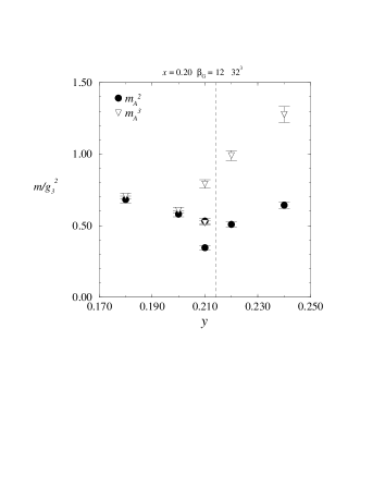
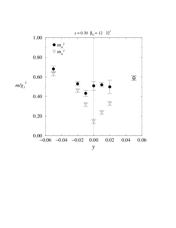
Figure 7: The screening masses of the scalar operators ${\rm Tr\,}A_{0}^{2}$ and ${\rm Tr\,}A_{0}^{3}$ at $x=0.2$ and 0.3. In the broken phase, both operators couple to the same states.

   

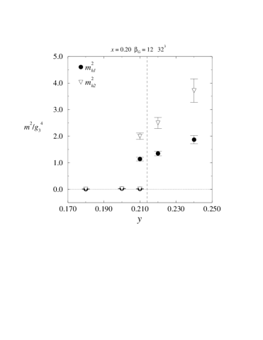
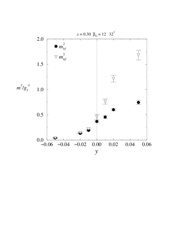
Figure 8: The screening masses squared of the vector operators $h_{1}={\rm Tr\,}A_{0}F_{12}$ and $h_{2}={\rm Tr\,}A^{2}_{0}F_{12}$ at $x=0.2$ and 0.3. In the broken phase, both operators couple to the same states.

The spatial correlation lengths, or inverse screening masses, were measured with a method using recursive levels of smearing and blocking of the gauge and $A_{0}$ variables. We used up to 4 blocking levels, which gives $2^{4}$ as the largest spatial extent of the operators. For technical details, we refer to [4].

In Figs. 7 and 8 we show the screening masses of the scalar operators ${\rm Tr\,}A_{0}^{2}$ and ${\rm Tr\,}A_{0}^{3}$ and the vector operators

$$h_{1,i}=\epsilon_{ijk}{\rm Tr\,}A_{0}F_{jk}\mbox{~{}~{}~{}~{}and~{}~{}~{}~{}}h_{2,i}=\epsilon_{ijk}{\rm Tr\,}A^{2}_{0}F_{jk}$$ (31)

at $x=0.20$ and 0.30. In the symmetric phase, ${\rm Tr\,}A_{0}^{2}$, ${\rm Tr\,}A_{0}^{3}$ have different quantum numbers and thus couple to different states; the same is true for $h_{1},h_{2}$. However, in the broken $A_{0}$ phase the operators can couple to each other, and should thus project to the same states. This is indeed observed in Fig. 7 within the statistical errors for $x=0.20$. For $x=0.30$ the signal of the ${\rm Tr\,}A_{0}^{2}$ correlator is quite noisy (and the errorbars do not contain any estimates of the systematic effects), but the pattern should be the same. Note that this does not as such imply that there would be a discontinuity in the mass spectrum at $y=y_{c},x=0.30$: it is just that in the broken phase ${\rm Tr\,}A_{0}^{2},{\rm Tr\,}A_{0}^{3}$ couple to the same excitations, and to determine the mass of the first exited state would require a mixing analysis, such as in [24]. In the symmetric phase, in contrast, ${\rm Tr\,}A_{0}^{2},{\rm Tr\,}A_{0}^{3}$ automatically couple to different states.

The scalar operator ${\rm Tr\,}A_{0}^{3}$ becomes “critical” at $x=0.30$: it approaches zero at $y=y_{c}$, as much as allowed by the finite volume. This is in accordance with the interpretation that ${\rm Tr\,}A_{0}^{3}$ acts like the magnetization of the 3d Ising model. A precise finite size scaling analysis of the critical correlation length is beyond the scope of this paper, and we rather interpret the right panel of Fig. 7 as a consistency check.

In perturbation theory, there always remains an unbroken U(1) gauge symmetry in the broken phase. The vector operators $h_{1}$ and $h_{2}$ couple to the massless U(1) “photons” $\gamma$. However, these photons become massive due to the interactions with Polyakov monopoles. Since we expect the screening mass to be very light, we measure it at non-zero transverse momentum: we use the operator

$$O_{1}(x_{3})={\frac{1}{N^{2}}}\sum_{x_{1},x_{2}}{\rm Tr\,}A_{0}F_{12}e^{i2\pi x_{1}/N}$$ (32)

and correspondingly for $h_{2}$ (on the lattice, ${\rm Tr\,}A_{0}F_{12}\to{\rm Tr\,}A_{0}U_{12}$). The screening mass is then measured from the asymptotic behaviour of the correlation function,

$$\langle O_{1}(x_{3})O_{1}(0)\rangle\propto\exp\Bigl{(}-x_{3}\sqrt{(2\pi/N)^{2}+m^{2}_{h_{1}}}\Bigr{)}\,.$$ (33)

The results are shown in Fig. 8. When $x=0.2$, the transition is strong and, within the statistical accuracy, the masses fall to zero in the broken phase. However, at $x=0.3$ the masses remain finite even in the broken phase. Due to the analytic continuation this implies that also at $x=0.2$ the masses are still finite; they are just too small to be observed.

It is interesting to note that the vector masses seem to vary rather smoothly when going from the symmetric to the broken phase, despite the fact that there is a true symmetry breaking phase transition. In fact, their behaviour is quite similar to that in the SU(2) + adjoint Higgs theory [4], where no transition at all is observed at large $x$ [13].

6 Conclusions

We have numerically determined the phase diagram of the 3d SU(3) + adjoint Higgs theory. We find a symmetric phase with $\langle{\rm Tr\,}A_{0}^{2}\rangle\approx 0$, $\langle{\rm Tr\,}A_{0}^{3}\rangle=0$, and a broken phase with $\langle{\rm Tr\,}A_{0}^{2}\rangle,\langle{\rm Tr\,}A_{0}^{3}\rangle$ non-vanishing and large. These are separated by a transition line which contains a first order regime, a second order regime, and a tricritical point in between. We did not observe any other types of phases.

From the statistical physics point of view, these results are of interest as a new qualitative class in the types of critical behaviours that have been found in 3d SU($N$)+Higgs theories. (It should be noted that even more classes could appear when external constraints such as a magnetic field are added, or when the Higgses are replaced by fermions [25] – the latter case is not relevant for finite temperature 4d theories, though. It can also be noted that a similar tricritical structure as found here can arise when there are several (fundamental) Higgses in the theory, related by a global symmetry [26].) It would be interesting to apply methods similar to those in [11] to a more precise study of the properties of the tricritical point. To our knowledge, the universal forms of the different probability distributions at the tricritical point have not been previously determined numerically in three-dimensional theories.

From the QCD point of view, we re-emphasize the fact that even though the SU(3) + adjoint Higgs theory has the phase structure given in this paper, only the symmetric phase is an accurate effective theory for the 4d finite temperature theory, permitting, say, the determination of static correlation functions. In particular, the phase transition of the effective theory is not that of the 4d theory. (Nevertheless, it is amusing to note that the location of the tricritical point $x_{c}$ corresponds to $T\approx 0.57\Lambda_{\overline{\rm MS}}$ according to 2-loop dimensional reduction, not far from the 4d transition temperature $T_{c}\approx 1.03\Lambda_{\overline{\rm MS}}$ [27].) One may also note that in the context of finite $T$ QCD it has been suggested [28] that the critical line in the $(T,\mu)$-plane for two massless flavours would have a similar tricritical structure. This clearly is not related to the tricritical structure studied here.

Finally, from the point of view of the finite temperature SU(5) theory, the present SU(3) case shows that only some of the possible broken phases are dynamically realized. It should be interesting to see how this statement is modified in the SU(5) case, where there is a wider spectrum of possibilities.

References

- [1] P. Ginsparg, Nucl. Phys. B 170 (1980) 388; T. Appelquist and R. Pisarski, Phys. Rev. D 23 (1981) 2305; S. Nadkarni, Phys. Rev. D 27 (1983) 917.
- [2] T. Reisz, Z. Phys. C 53 (1992) 169; L. Kärkkäinen, P. Lacock, D.E. Miller, B. Petersson and T. Reisz, Phys. Lett. B 282 (1992) 121; Nucl. Phys. B 418 (1994) 3; L. Kärkkäinen, P. Lacock, B. Petersson and T. Reisz, Nucl. Phys. B 395 (1993) 733.
- [3] E. Braaten and A. Nieto, Phys. Rev. Lett. 76 (1996) 1417 [hep-ph/9508406]; Phys. Rev. D 53 (1996) 3421 [hep-ph/9510408]; A. Nieto, Int. J. Mod. Phys. A 12 (1997) 1431 [hep-ph/9612291].
- [4] K. Kajantie, M. Laine, K. Rummukainen and M. Shaposhnikov, Nucl. Phys. B 503 (1997) 357 [hep-ph/9704416].
- [5] S. Dutta and S. Gupta, hep-lat/9806034.
- [6] A. Rajantie, Nucl. Phys. B 501 (1997) 521 [hep-ph/9702255].
- [7] S. Bronoff, R. Buffa and C. Korthals Altes, hep-ph/9809452.
- [8] K. Kajantie, M. Laine, K. Rummukainen and M. Shaposhnikov, Phys. Rev. Lett. 77 (1996) 2887 [hep-ph/9605288].
- [9] F. Karsch, T. Neuhaus, A. Patkós and J. Rank, Nucl. Phys. B (Proc. Suppl.) 53 (1997) 623 [hep-lat/9608087].
- [10] M. Gürtler, E.-M. Ilgenfritz and A. Schiller, Phys. Rev. D 56 (1997) 3888 [hep-lat/9704013].
- [11] K. Rummukainen, M. Tsypin, K. Kajantie, M. Laine and M. Shaposhnikov, Nucl. Phys. B, in press [hep-lat/9805013].
- [12] K. Kajantie, M. Laine, K. Rummukainen and M. Shaposhnikov, Nucl. Phys. B 493 (1997) 413 [hep-lat/9612006].
- [13] A. Hart, O. Philipsen, J.D. Stack and M. Teper, Phys. Lett. B 396 (1997) 217 [hep-lat/9612021].
- [14] B.I. Halperin, T.C. Lubensky and S.-K. Ma, Phys. Rev. Lett. 32 (1974) 292; C. Dasgupta and B.I. Halperin, Phys. Rev. Lett. 47 (1981) 1556; J. Bartholomew, Phys. Rev. B 28 (1983) 5378; Y. Munehisa, Phys. Lett. B 155 (1985) 159; P. Dimopoulos, K. Farakos and G. Kotsoumbas, Eur. Phys. J. C 1 (1998) 711 [hep-lat/9703004]; K. Kajantie, M. Karjalainen, M. Laine and J. Peisa, Phys. Rev. B 57 (1998) 3011 [cond-mat/9704056]; Nucl. Phys. B 520 (1998) 345 [hep-lat/9711048].
- [15] P. Arnold and L.G. Yaffe, Phys. Rev. D 52 (1995) 7208 [hep-ph/9508280].
- [16] K. Kajantie, M. Laine, K. Rummukainen and M. Shaposhnikov, Phys. Lett. B 423 (1998) 137 [hep-ph/9710538].
- [17] M. Laine and A. Rajantie, Nucl. Phys. B 513 (1998) 471 [hep-lat/9705003].
- [18] G.D. Moore, Nucl. Phys. B 493 (1997) 439 [hep-lat/9709053].
- [19] K. Farakos, K. Kajantie, K. Rummukainen and M. Shaposhnikov, Nucl. Phys. B 442 (1995) 317 [hep-lat/9412091].
- [20] T. Toimela, Phys. Lett. B 124 (1983) 407.
- [21] F.Y. Wu, Rev. Mod. Phys. 54 (1982) 235; R.V. Gavai, F. Karsch and B. Petersson, Nucl. Phys. B 322 (1989) 738; M.A. Stephanov and M.M. Tsypin, Nucl. Phys. B 366 (1991) 420.
- [22] K. Kajantie, M. Laine, J. Peisa, A. Rajantie, K. Rummukainen and M. Shaposhnikov, Phys. Rev. Lett. 79 (1997) 3130 [hep-ph/9708207].
- [23] R. Guida and J. Zinn-Justin, cond-mat/9803240.
- [24] O. Philipsen, M. Teper and H. Wittig, Nucl. Phys. B 469 (1996) 445 [hep-lat/9602006].
- [25] K. Farakos, N.E. Mavromatos and D. McNeill, hep-lat/9806029.
- [26] P. Arnold and D. Wright, Phys. Rev. D 55 (1997) 6274 [hep-ph/9610226].
- [27] J. Fingberg, U. Heller and F. Karsch, Nucl. Phys. B 392 (1993) 493.
- [28] A. Barducci, R. Casalbuoni, G. Pettini and R. Gatto, Phys. Rev. D 49 (1994) 426; J. Berges and K. Rajagopal, hep-ph/9804233; M.A. Halasz, A.D. Jackson, R.E. Shrock, M.A. Stephanov and J.J.M. Verbaarschot, Phys. Rev. D 58 (1998) 096007 [hep-ph/9804290]; M. Stephanov, R. Rajagopal and E. Shuryak, hep-ph/9806219.