On the Neuberger overlap operator

Abstract

We compute Neuberger’s overlap operator by the Lanczos algorithm applied to the Wilson-Dirac operator. Locality of the operator for quenched QCD data and its eigenvalue spectrum in an instanton background are studied.

PACS No.: 11.15Ha, 11.30.Rd, 11.30.Fs

Key Words: Lattice QCD, Chiral fermions, Algorithms

1. Although brute force calculations of the quenched lattice QCD with Wilson fermions have been able to approach the chiral limit [1], there are increased efforts to make the chiral symmetry exact on the lattice [2, 3].

There are different starting points to formulate lattice actions with exact lattice chiral symmetry, but all of them seem to obey the Ginsparg-Wilson condition [5]:

$$\gamma_{5}D^{-1}+D^{-1}\gamma_{5}=a\gamma_{5}{\alpha}^{-1},$$ (1)

where $a$ is the lattice spacing, $D$ is the lattice Dirac operator and ${\alpha}^{-1}$ is a local operator and trivial in the Dirac space.

A candidate is the overlap operator of Neuberger [6]:

$$D=1-\gamma_{5}\mbox{sign}(H),~{}~{}~{}~{}H=\gamma_{5}(\sigma-aD_{W})$$ (2)

where $\sigma$ is a shift parameter in the range $(0,2)$, which we have fixed at one and $D_{W}$ is the Wilson-Dirac operator,

$$D_{W}=\frac{1}{2}\sum_{\mu}[\gamma_{\mu}(\partial_{\mu}^{*}+\partial_{\mu})-a\partial_{\mu}^{*}\partial_{\mu}]$$ (3)

and $\partial_{\mu}$ and $\partial_{\mu}^{*}$ are the nearest-neighbor forward and backward difference operators.

The locality has been shown for smooth background fields and no violation has been observed in quenched samples simulated at moderate couplings [7].

2. So far, all the methods devised to compute the overlap operator by usual iterative solvers have been based on (rational) polynomial approximations of the inverse square root or the $sign$ function [8, 9]. (Mathematical foundations of these methods are reviewed in [10].) But they may exceed the storage limits in some machines. This is not the case with Legendre [11] and Chebyshev [7] polynomials, which on the other hand are not optimal [12].

In the present work we propose a new method, which uses the outcome of the Lanczos algorithm on $H$. The Lanczos iteration is known to approximate the spectrum of the underlying matrix in an optimal way and, in particular, it requires a constant memory [14].

Let $Q_{n}=[q_{1},\ldots,q_{n}]$ be the set of orthonormal vectors, such that

$$HQ_{n}=Q_{n}T_{n},~{}~{}~{}~{}q_{1}=\rho_{1}b,~{}~{}~{}~{}\rho_{1}=1/||b||_{2}$$ (4)

where $T_{n}$ is a tridiagonal and symmetric matrix. Here $b$ stands for an arbitrary vector.

By writing down the above decomposition in terms of the vectors $q_{i},i=1,\ldots,n$ and the matrix elements of $T_{n}$, we arrive at a three term recurrence that allows to compute these vectors in increasing order, starting from the vector $q_{1}$. This is called the Lanczos algorithm, which constructs a basis for the so called Krylov subspace: $span(b,Hb,\ldots,H^{n-1}b)$ [14].

In the last equation, it has been assumed that after $n$ steps of the Lanczos algorithm, the Krylov subspace remains invariant. The task is the computation of $x=(H^{2})^{-1/2}b$. Our method is based on the following observations: Let $(H^{2})^{-1/2}=f(H^{2})$ be a matrix-valued function, for example Robert’s integral formula [10]:

$$f(H^{2})=\frac{2}{\pi}\int_{0}^{\infty}dt(t^{2}+H^{2})^{-1}$$ (5)

Then, clearly:

$$f(H^{2})Q_{n}=Q_{n}f(T_{n}^{2})$$ (6)

Since, on the other hand,

$$b=Q_{n}e_{1}^{(n)}/\rho_{1},$$ (7)

where $e_{1}^{(n)}$ denotes the unit vector with $n$ elements in the direction $1$, we get:

$$x=f(H^{2})b=Q_{n}f(T_{n}^{2})e_{1}^{(n)}/\rho_{1}$$ (8)

There are some remarks to be made here:

a) By applying the Lanczos iteration on $H$, the problem of computing $(H^{2})^{-1/2}$ reduces to the problem of computing $(T_{n}^{2})^{-1/2}$ which is typically a much smaller problem than the original one. It can be solved for example by using the full decomposition of $T_{n}$ in its eigenvalues and eigenvectors; in fact this is the method we have employed too, for its compactness and the small overhead for moderate $n$.

b) In the floating point arithmetic, there is a danger that once the Lanczos polynomial (algorithm) has approximated well some part of the spectrum, the iteration reproduces vectors which are rich in that direction [15]. As a consequence, the orthogonality of the Lanczos vectors is spoiled with an immediate impact on the history of the iteration.

c) In general, there is no guarantee that the algorithm will converge at smaller $n$, unless $n=\mbox{rank}(H)$ in exact arithmetic [14]. Therefore, for a given $n$ the equations (4) and (8) hold approximately.

Therefore, in practical implementations one should be satisfied with a stopping criterium such as:

$$\mbox{error}(n)=|(\rho_{1}||Hx_{n}||_{2})^{2}-1|^{1/2}$$ (9)

is made small enough.

It is worth writing down the error in terms of the Lanczos matrix; straightforward algebra gives:

$$\mbox{error}(n)=|\beta_{n}z_{n}^{(n)}|,~{}~{}~{}~{}z_{n}=(T_{n}^{2})^{-1/2}e_{1}^{(n)}$$ (10)

where $\beta_{n}$ is the element $(n+1,n)$ of the matrix $T_{n+1}$ and $z_{n}^{(n)}$ is the last component of the vector $z_{n}$.

Since $H$ and $(H^{2})^{1/2}$ are equally conditioned in 2-norm, we expect, that once the system $Hx=b$ is solved, the system $(H^{2})^{1/2}x=b$ is also solved. In this context, it is desirable to compare the error (10) with the residual error of the original system, $r_{n}$. As before, in terms of the Lanczos matrix, it is given by:

$$||\rho_{1}r_{n}||_{2}=|\beta_{n}y_{n}^{(n)}|,~{}~{}~{}y_{n}=T_{n}^{-1}e_{1}^{(n)}$$ (11)

As long as the orthogonality between Lanczos vectors is sufficiently maintained, equations (10-11) should hold to a good accuracy.

To implement the result (8), we first construct the Lanczos matrix and then compute $z_{n}$. By repeating the iteration, we compute Lanczos vectors and obtain the result. We saved the scalar products, though it was not necessary. If we call $1/\rho_{i},i=1,\ldots$ the norm of the residual error of the system $Hx=b$, it is easy to show that

$$\rho_{i+1}\beta_{i}+\rho_{i}\alpha_{i}+\rho_{i-1}\beta_{i-1}=0$$ (12)

Therefore, we have the following algorithm for solving the system $(H^{2})^{1/2}x=b$:

$$\begin{array}[]{l}\beta_{0}=0,~{}\rho_{1}=1/||b||_{2},~{}q_{0}=o,~{}q_{1}=\rho_{1}b\\ for~{}i=1,\ldots\\ ~{}~{}~{}~{}v=Hq_{i}\\ ~{}~{}~{}~{}\alpha_{i}=q_{i}^{{\dagger}}v\\ ~{}~{}~{}~{}v:=v-q_{i}\alpha_{i}-q_{i-1}\beta_{i-1}\\ ~{}~{}~{}~{}\beta_{i}=||v||_{2}\\ ~{}~{}~{}~{}q_{i+1}=v/\beta_{i}\\ ~{}~{}~{}~{}\rho_{i+1}=-\frac{\rho_{i}\alpha_{i}+\rho_{i-1}\beta_{i-1}}{\beta_{i}}\\ ~{}~{}~{}~{}if\frac{1}{|\rho_{i+1}|}<tol,~{}n=i,~{}end~{}for\\ \\ Set~{}(T_{n})_{i,i}=\alpha_{i},~{}(T_{n})_{i+1,i}=(T_{n})_{i,i+1}=\beta_{i},otherwise~{}(T_{n})_{i,j}=0\\ z_{n}=(T_{n}^{2})^{-1/2}=U_{n}(\Lambda_{n}^{2})^{-1/2}U_{n}^{T}e_{1}^{(n)}\\ \\ q_{0}=o,~{}q_{1}=\rho_{1}b,~{}x_{0}=o\\ for~{}i=1,\ldots,n\\ ~{}~{}~{}~{}x_{i}=x_{i-1}+q_{i}z_{n}^{(i)}/\rho_{1}\\ ~{}~{}~{}~{}v=Hq_{i}\\ ~{}~{}~{}~{}v:=v-q_{i}\alpha_{i}-q_{i-1}\beta_{i-1}\\ ~{}~{}~{}~{}q_{i+1}=v/\beta_{i}\\ \end{array}$$ (13)

where by $o$ we denote a vector with zero entries and $U_{n},\Lambda_{n}$ the matrices of the egienvectors and eigenvalues of $T_{n}$. Note that there are only four large vectors necessary to store: $q_{i-1},q_{i},v,x_{i}$.

Obviously, the memory doesn’t grow with $n$. This is not the case for the shifted CG iterations ([8, 9]) needed to compute the (rational) polynomial approximation of $(H^{2})^{-1/2}$. Since there is a one to one connection between CG and Lanczos, such approximations on the original matrix are transfered to the corresponding Lanczos matrix [14]. This should be contrasted with the exact computation of $(T_{n}^{2})^{-1/2}$.

To test the above analysis, we have performed simulations of SU(3) gauge theory at $\beta=6.0$ on a $8^{3}16$ lattice and picked up an equilibrated configuration.

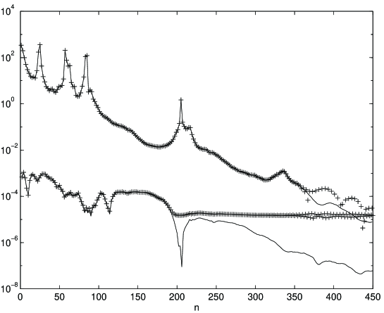
Figure 1: Residual error of the system $(H^{2})^{1/2}x=b$ as defined in (9): plus symbols that jump between two branches. The same quantity defined in terms of the Lanczos matrix is displayed by the solid line.

In Fig.1 we show the residual error $|(\rho_{1}||Hx_{n}||_{2})^{2}-1|^{1/2}$ computed directly from $x_{n}$ and compare with the same quantity given in terms of the Lanczos matrix, i.e. $|\beta_{n}z_{n}^{(n)}|$. It fluctuates between two branches: the upper one corresponds to odd $n$, the number of matrix-vector multiplications, and the lower one to even values of $n$. For large $n$, the computed and estimated errors deviate from each other, which may indicate accumulation of roundoff errors in the computed residual error. Note that we have employed 64 bit precision.

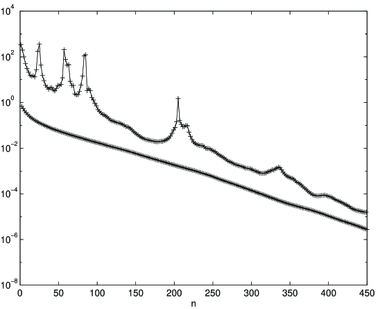
Figure 2: Residual error of the system $Hx=b$: plus symbols that jump between two branches. The same quantity defined in terms of the Lanczos matrix is displayed by the solid line.

For comparison, we show in Fig.2 the residual error $||\rho_{1}r_{n}||_{2}$ of the system $Hx=b$ as computed directly and from $|\beta_{n}y_{n}^{(n)}|$. Again, we have two branches as explained above, but here there is no distinction between the computed and estimated errors. The appearance of two branches is not surprising since we are dealing with a non-definite matrix $H$.

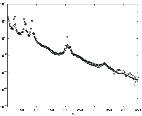
Figure 3: Residual error of the systems $Hx=b$ (plus symbols) and $(H^{2})^{1/2}x=b$ (circle symbols) for odd $n$.

In Fig.3 we compare the computed residual errors of the systems $Hx=b$ and $(H^{2})^{1/2}x=b$ (upper branches). They are the same most of the time, unless $n$ becomes large and deviations become clearer. This behavior shows that both systems are solved at the same time, which should serve us as a guide, because the computation of $x_{i}$ at each step $i$ is very demanding.

We have compared the efficiency of the above method with that of the rational polynomial approximation [8]. First, we solved the system $Hx=b$ by both Lanczos and CG with an $10^{-5}$ accuracy for the residual error. We needed the same number of multiplications with $H^{2}$, 226. To compute the inverse square root with the same accuracy ($10^{-5}$), we applied then the above method and the rational polynomial method with $N=30$, the number of the terms in the approximating sum ([8]). (Smaller $N$ will give a lower accuracy: in Fig. 4 we display the norm of the residual error (9) as a function of $N$.) Therefore, if we stored the Lanczos vectors as in the rational polynomial method, both methods need about the same amount of work. To avoid memory restrictions, we increase the work by a factor of two.

3. An immediate application of the above method is to check the locality of Neuberger’s overlap operator $D$.

We used 100 equilibrated SU(3) configurations at $\beta=5.7,6.0$ on a $8^{3}16$ lattice. For each configuration we computed the absolute value of $D$ elements in the first column with space, spin and color indices fixed at one, a selection that suffices to look for violations of the locality.

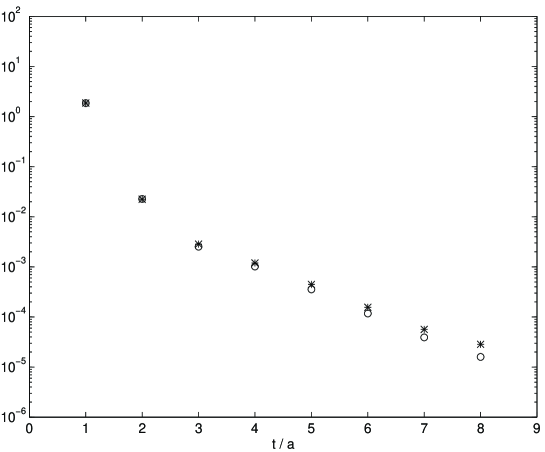
Figure 5: Absolute value of $D$ elements in the first column with space, spin and color indices fixed at one, as a function of time indices at $\beta=6.0$ (circles) and $\beta=5.7$ (stars).

The average over 100 configurations is plotted in Fig. 5. At both values of $\beta$, there was no single configuration to show an exceptional behavior: the maximum deviation is slightly above the mean value. The values of $D$ decrease rapidly with the time slices. For large $t/a$ but away from the center, they fall off exponentially.

Recently, it has been shown that for $\beta=6.0,6.2,6.4$ the occurrence of configurations with exceptionally small eigenvalues of $H^{2}$ becomes vanishingly small for $12^{4}$ and $16^{4}$ large lattices, whereas for sufficiently smooth gauge fileds the locality is guaranteed [7].

In fact at $\beta=5.7$ the complete spectrum of $1-D_{W}$ is in the left half of the complex plane. We computed partial spectra of $\gamma_{5}H$ by the implicitely restarted Arnoldi iteration [17] and found that indeed at this coupling there was no eigenvalue in the right half of the complex plane for all our 100 configurations. Therefore, there exist a $\beta\in(5.7,6.0)$ at which the operator $1-D_{W}$ becomes singular. In this case, there is an unbounded number of near zero modes of $H$ and therefore $D$ is no longer local.

4. As another application we consider the lattice index theorem for an SU(2) instanton background on a small $4^{4}$ lattice. An instanton on the lattice can be prepared in various ways. We follow [18] and prepare an instanton with size $\rho$ in the center of the lattice in the singular gauge. The index of $D$ is given by:

$$\mbox{index}(D)=\frac{1}{2}\mbox{Tr}[\mbox{sign}(H)]$$ (14)

Because of the O(a) lattice errors, we expect the instanton being observed for $\rho\geq a$. We computed the smallest eigenvalues of $D$ by an (implicitly restarted) Arnoldi iteration with the non-converged Ritz values used as explicit shifts [17]. We fixed the number of Arnoldi steps at 32 and have stopped the iteration when the next starting vector norm is smaller than $10^{-6}$. We have checked the stability of the computed eigenvalues by increasing the cutoff beyond the number of the converged eigenvalues. The stability is observed unless the cutoff becomes too large, which means that a larger Arnoldi matrix should be employed.

We note that it is crucial for the eigenvalue computation to have a proper accuracy in the computation of $D$, which in our case has been set at a residual error norm (9) less than $10^{-10}$.

We have computed eigenvalues for $\rho/a\in[0.5,1.5]$ with steps of $0.1$. For brevity, we show in Table 1 eigenvalues of a smaller set of $\rho$. For $\rho\leq a$ there are two zero modes, whereas for $\rho>a$ there is a single zero mode present. As numerical accuracy is an issue here, we have perturbed the instanton background by applying a small fluctuating gauge field. The picture doesn’t change, but the zero modes for $\rho\leq a$ become nearly zero modes with opposite chiralities.

We have also computed the eigenvalues exactly by standard QR algorithms. The instanton mode appears single in both approaches. While the values of the other smallest eigenvalues are reproduced exactly by the implicitly restarted Arnoldi algorithm, their multiplicity cannot be handled. Since $D$ is normal, the Arnoldi matrix is normal and tridiagonal and therefore irreducible, giving no information on the multiplicity. The latter is essential when $D$ has more exact zero modes and one must rely on block variants of the same algorithm.

Even on such a small lattice, the computation of the zero modes is not the fastest method to compute the topological charge. Tracing the crossings of the smallest eigenvalues of $H$ is more practical.

Nonetheless we note that an estimation of the topological charge can be made during the computation of $D$ as described in this work. Having computed the Lanczos matrix of $H$ one can estimate sign($H$), which for our SU(2) instanton gives excellent agreement for most of starting vectors $b$. In general, a separate study is needed to conclude on this method.

5. To conclude: we have computed with a new method the overlap operator based on the Lanczos algorithm applied on the Wilson-Dirac operator. Compared to the other methods [8, 9], its main advantage is of being free from memory restrictions. Additionally, there is no approximation made in the computation of the inverse square root of the Lanczos matrix.

The locality of the overlap operator has been tested. We recommend to check it always before any other computation.

The computation of $D$ turns to be more difficult than $D_{W}$. However, the so-called classically perfect actions [4] may help substantially to work on moderate lattices. Further studies are needed for the dynamical implementation of $D$.

We are grateful to stimulating discussions with Ferenc Niedermayer on the topics covered by this work and to Roland Rosenfelder and Philippe de Forcrand for making critical remarks on this paper.

We are grateful to Herbert Neuberger for comments on the method presented in this work following the posting of its first version.

We thank PSI where this work was done and SCSC Manno for the allocation of computer time on the NEC SX4.

Figure 4: Residual error of the system $(H^{2})^{1/2}x=b$ as a function of $N$ in the rational polynomial approximation.

$\rho$ = 0.9a	$\rho$ = 1.0a	$\rho$ = 1.1a
		0.277E -11+i0.660E -13
0.124E -12 -i0.198E -14	0.572E -11 -i0.694E -11	0.303E+00 -i0.717E+00
0.955E -11+i0.167E -13	0.575E -11+i0.697E -11	0.303E+00+i0.717E+00
0.947E+00 -i0.998E+00	0.940E+00 -i0.998E+00	0.303E+00 -i0.717E+00
0.947E+00+i0.998E+00	0.940E+00+i0.998E+00	0.303E+00+i0.717E+00
0.957E+00 -i0.997E+00	0.950E+00 -i0.995E+00	0.931E+00 -i0.997E+00
0.957E+00+i0.997E+00	0.950E+00+i0.995E+00	0.931E+00+i0.997E+00
0.102E+01 -i0.999E+00	0.102E+01 -i0.999E+00	0.939E+00 -i0.997E+00
0.102E+01+i0.999E+00	0.102E+01+i0.999E+00	0.939E+00+i0.997E+00
0.104E+01 -i0.998E+00	0.104E+01+i0.997E+00	0.103E+01 -i0.998E+00
0.104E+01+i0.998E+00	0.104E+01 -i0.997E+00	0.103E+01+i0.998E+00

Table 1: Smallest eigenvalues of $D$ for three instanton sizes $\rho$

References

- [1] R. Burkhalter for the CP-PACS Collaboration, Recent Results from the CP-PACS Collaboration, UTCCP-P-52, Oct. 1998, and hep-lat/9810043.
- [2] R. Narayanan, H. Neuberger, Phys. Lett. B 302 (1993) 62, Nucl. Phys. B 443 (1995) 305.
- [3] P. Hasenfratz, V. Laliena and F. Niedermayer, Phys. Lett. B 427 (1998) 125, M. Lüscher, Phys. Lett. B 428 (1998) 342.
- [4] F. Niedermayer, Exact chiral symmetry, topological charge and related topics, hep-lat/9810026.
- [5] P. H. Ginsparg and K. G. Wilson, Phys. Rev. D 25 (1982) 2649.
- [6] H. Neuberger, Phys. Lett. B 417 (1998) 141, Phys. Rev. D 57 (1998) 5417.
- [7] P. Hernández, K. Jansen and M. Lüscher, CERN-TH/98-250, DESY 98-094, and hep-lat/9808010.
- [8] H. Neuberger, Phys. Rev. Lett. 81 (1998) 4060.
- [9] R. G. Edwards, U. M. Heller and R. Narayanan, A study of practical implementations of the Overlap-Dirac operator in four dimensions, FSU-SCRI-98-71, and hep-lat/9807017.
- [10] N. J. Higham, Proceedings of ”Pure and Applied Linear Algebra: The New Generation”, Pensacola, March 1993.
- [11] B. Bunk, Nucl.Phys.Proc.Suppl. B63 (1998) 952.
- [12] While Legendre polynomials are not optimal in any sense here, Chebyshev polynomials are not optimal in the sense that their roots do not represent the actual distribution of the eigenvalues of [14].
- [13] H. Neuberger, hep-lat/9811019.
- [14] G. H. Golub and C. F. Van Loan, Matrix Computations, The Johns Hopkins University Press, Baltimore, 1989.
- [15] H. D. Simon, Linear Algebra and its Applications 61:101-131(1984).
- [16] F. Butler, et al., Nucl. Phys. B 430 (1994) 179.
- [17] D. C. Sorensen, SIAM J. Matrix Anal. Appl. 13 (1992), 357-385.
- [18] M. L. Laursen, J. Smit and J. C. Vink, Nucl. Phys. B 343 (1990) 522.