DESY 98-165
Evidence for discrete chiral symmetry breaking
in $N=1$ supersymmetric Yang-Mills theory

Abstract

In a numerical Monte Carlo simulation of SU(2) Yang-Mills theory with dynamical gauginos we find evidence for two degenerate ground states at the supersymmetry point corresponding to zero gaugino mass. This is consistent with the expected pattern of spontaneous discrete chiral symmetry breaking $Z_{4}\to Z_{2}$ caused by gaugino condensation.

1 Introduction

The basic assumption about the non-perturbative dynamics of supersymmetric Yang-Mills (SYM) theory is that there is confinement and spontaneous chiral symmetry breaking, similar to QCD [1]. (For a more recent introduction and review see also [2].) In the past years there has been great progress in the understanding of the non-perturbative properties of supersymmetric gauge theories, in particular following the seminal papers of Seiberg and Witten [3]. In case of $N=1$ SYM theory the non-perturbative results are not rigorous but fit into a self-consistent plausible picture of low energy dynamics of supersymmetric QCD (SQCD) [4]. The features of the low energy dynamics, like symmetries and bound state spectra, are formulated in terms of low energy effective actions [5, 6]. Lattice Monte Carlo simulations may contribute by directly testing some of these predictions.

The expected pattern of spontaneous chiral symmetry breaking in SYM theories is quite interesting: considering for definiteness the gauge group SU($N_{c}$), the expected symmetry breaking is $Z_{2N_{c}}\to Z_{2}$. This is because the global chiral symmetry of the gaugino (a Majorana fermion in the adjoint representation) is anomalous. The symmetry transformations are

$$\Psi_{x}\to e^{-i\varphi\gamma_{5}}\Psi_{x}\ ,\hskip 20.00003pt\bar{\Psi}_{x}\to\bar{\Psi}_{x}e^{-i\varphi\gamma_{5}}\ ,$$ (1)

where the Dirac-Majorana fields are used which satisfy, with the charge-conjugation Dirac matrix $C$,

$$\Psi_{x}=C\overline{\Psi}_{x}\ ,\hskip 20.00003pt\overline{\Psi}_{x}=\Psi_{x}^{T}C\ .$$ (2)

The group of symmetry transformations in (1) coincide with the $R$-symmetry and hence will be called ${\rm U(1)}_{R}$. The transformation is equivalent to the transformation of the gaugino mass $m_{\tilde{g}}$ and a shift of the $\theta$-parameter:

$$m_{\tilde{g}}\to m_{\tilde{g}}e^{-2i\varphi\gamma_{5}}\ ,\hskip 20.00003pt\theta\to\theta-2N_{c}\varphi\ .$$ (3)

Since $\theta$ is periodic with period $2\pi$, in the supersymmetric case with $m_{\tilde{g}}=0$ the ${\rm U(1)}_{R}$ symmetry is unbroken if

$$\varphi=\varphi_{k}\equiv\frac{k\pi}{N_{c}}\ ,\hskip 20.00003pt(k=0,1,\ldots,2N_{c}-1)\ .$$ (4)

Gaugino condensation means a non-zero vacuum expectation value

$$\langle\bar{\Psi}_{x}\Psi_{x}\rangle=\langle\lambda_{x}^{\alpha}\lambda_{x\alpha}+\bar{\lambda}_{x}^{\dot{\alpha}}\bar{\lambda}_{x\dot{\alpha}}\rangle\neq 0\ .$$ (5)

(Here, besides the Dirac-Majorana field, the Weyl-Majorana field components $\lambda_{x}^{\alpha}$ and $\bar{\lambda}_{x}^{\dot{\alpha}}$ are also introduced.) The gaugino condensate is transformed under ${\rm U(1)}_{R}$ according to

$$\langle\bar{\Psi}_{x}\Psi_{x}\rangle\to\langle\bar{\Psi}_{x}e^{-2i\varphi\gamma_{5}}\Psi_{x}\rangle\ .$$ (6)

If such a condensate is produced by the dynamics then it breaks the $Z_{2N_{c}}$ symmetry to $Z_{2}$: the expected spontaneous chiral symmetry breaking is $Z_{2N_{c}}\to Z_{2}$. This implies the existence of $N_{c}$ discrete degenerate ground (vacuum) states with different orientations of the gaugino condensate according to (4), (6).

A non-zero gaugino mass ($m_{\tilde{g}}\neq 0$) breaks the supersymmetry softly. As a function of the gaugino mass the degeneracy of the $N_{c}$ ground states is resolved. At $m_{\tilde{g}}=0$ the lowest ground state is changing. This gives rise to a characteristic pattern of first order phase transitions.

In the special case of SU(2) gauge group, which will be considered in this paper, we have $Z_{4}\to Z_{2}$ and in the two vacua the gaugino condensate has opposite signs. At $m_{\tilde{g}}=0$ the lowest ground states are exchanged and a first order phase transition occurs. In this letter we report on a large scale numerical Monte Carlo simulation with the aim to find numerical evidence for the existence of this phase transition.

2 Lattice formulation

The definition of an Euclidean path integral for Majorana fermions [7] may be obtained by starting from the well known Wilson formulation [8] of a Dirac fermion in the adjoint representation. If the Grassmanian fermion fields in the adjoint representation are denoted by $\psi^{r}_{x}$ and $\overline{\psi}^{\ r}_{x}$, with $r$ being the adjoint representation index, then the fermionic part of the lattice action can be written as

$$S_{f}=\sum_{xu,yv}\overline{\psi}^{\ v}_{y}Q_{yv,xu}\psi^{u}_{x}\ .$$ (7)

Here the fermion matrix $Q$ is defined by

$$Q_{yv,xu}\equiv Q_{yv,xu}[U]\equiv\delta_{yx}\delta_{vu}-K\sum_{\mu=1}^{4}\left[\delta_{y,x+\hat{\mu}}(1+\gamma_{\mu})V_{vu,x\mu}+\delta_{y+\hat{\mu},x}(1-\gamma_{\mu})V^{T}_{vu,y\mu}\right]\ .$$ (8)

$K$ is the hopping parameter and the matrix for the gauge-field link in the adjoint representation is defined as

$$V_{rs,x\mu}\equiv V_{rs,x\mu}[U]\equiv 2{\rm Tr}(U_{x\mu}^{\dagger}T_{r}U_{x\mu}T_{s})=V_{rs,x\mu}^{*}=V_{rs,x\mu}^{-1T}\ .$$ (9)

The generators $T_{r}\equiv\frac{1}{2}\lambda_{r}$ satisfy the usual normalization ${\rm Tr\,}(\lambda_{r}\lambda_{s})=\frac{1}{2}\delta_{rs}$. In case of SU(2) we have $T_{r}\equiv\frac{1}{2}\tau_{r}$ with the isospin Pauli-matrices $\tau_{r}$. Starting from the Dirac fermion fields one can introduce two Dirac-Majorana fields $\Psi^{(1,2)}$ satisfying (2):

$$\Psi^{(1)}\equiv\frac{1}{\sqrt{2}}(\psi+C\overline{\psi}^{T})\ ,\hskip 20.00003pt\Psi^{(2)}\equiv\frac{i}{\sqrt{2}}(-\psi+C\overline{\psi}^{T})$$ (10)

and $S_{f}$ can be rewritten as

$$S_{f}=\frac{1}{2}\sum_{j=1}^{2}\sum_{xu,yv}\overline{\Psi}^{(j)v}_{y}Q_{yv,xu}\Psi^{(j)u}_{x}\ .$$ (11)

Using this, the fermionic path integral for Dirac fermions becomes

$$\int[d\overline{\psi}d\psi]e^{-S_{f}}=\int[d\overline{\psi}d\psi]e^{-\overline{\psi}Q\psi}=\det Q=\prod_{j=1}^{2}\int[d\Psi^{(j)}]e^{-\frac{1}{2}\overline{\Psi}^{(j)}Q\Psi^{(j)}}\ .$$ (12)

For Majorana fields the path integral involves only $[d\Psi^{(j)}]$, either with $j=1$ or $j=2$ hence, omitting the index $(j)$, we have

$$\int[d\Psi]e^{-\frac{1}{2}\overline{\Psi}Q\Psi}=\int[d\Psi]e^{-\frac{1}{2}\Psi^{T}CQ\Psi}={\rm Pf}(CQ)={\rm Pf}(M)\ .$$ (13)

Here the Pfaffian of the antisymmetric matrix $M\equiv CQ$ is introduced. The Pfaffian can be defined for a general complex antisymmetric matrix $M_{\alpha\beta}=-M_{\beta\alpha}$ with an even number of dimensions ($1\leq\alpha,\beta\leq 2N$) by a Grassmann integral as

$${\rm Pf}(M)\equiv\int[d\phi]e^{-\frac{1}{2}\phi_{\alpha}M_{\alpha\beta}\phi_{\beta}}=\frac{1}{N!2^{N}}\epsilon_{\alpha_{1}\beta_{1}\ldots\alpha_{N}\beta_{N}}M_{\alpha_{1}\beta_{1}}\ldots M_{\alpha_{N}\beta_{N}}\ .$$ (14)

Here, of course, $[d\phi]\equiv d\phi_{2N}\ldots d\phi_{1}$, and $\epsilon$ is the totally antisymmetric unit tensor. It can be easily shown that

$$\left[{\rm Pf}(M)\right]^{2}=\det M\ .$$ (15)

One way to prove this is to use $\det M=\det CQ=\det Q$ and eqs. (12)-(13). Besides the partition function in (12), expectation values for Majorana fermions can also be similarly defined [9, 10].

It is easy to show [11] that the adjoint fermion matrix $Q$ has doubly degenerate real eigenvalues, therefore $\det Q$ is positive and ${\rm Pf}(M)$ is real. Omitting the sign of ${\rm Pf}(M)$ one obtains the effective gauge field action [12]:

$$S_{CV}=\beta\sum_{pl}\left(1-\frac{1}{2}{\rm Tr\,}U_{pl}\right)-\frac{1}{2}\log\det Q[U]\ ,$$ (16)

with the bare gauge coupling given by $\beta\equiv 2N_{c}/g^{2}$. The factor $\frac{1}{2}$ in front of $\log\det Q$ tells that we effectively have a flavour number $N_{f}=\frac{1}{2}$ of adjoint fermions. The omitted sign of the Pfaffian can be taken into account in the expectation values:

$$\langle A\rangle=\frac{\langle A\;{\rm sign\,Pf}(M)\rangle_{CV}}{\langle{\rm sign\,Pf}(M)\rangle_{CV}}\ .$$ (17)

This sign problem is very similar to the one in QCD with an odd number of quark flavours.

The value of the Pfaffian, hence its sign, can be numerically determined by calculating an appropriate determinant [13]. It turns out that in updating sequences with dynamical gauginos configurations with positive Pfaffian dominate. This is shown by explicit evaluation on $4^{3}\cdot 8$ lattices. It is plausible that the sign changes, as a function of the valence hopping parameter, typically occur at higher values than the value of $K$ in the dynamical updating [13]. Therefore, in the present work, we consider the effective gauge action in (16) and neglect the sign of the Pfaffian. To take into account the sign is possible but numerically demanding, therefore we postpone it for future studies.

Since the Monte Carlo calculations are done on finite lattices, one has to specify boundary conditions. In the three spatial directions we take periodic boundary conditions both for the gauge field and the gaugino. This implies that in the Hilbert space of states the supersymmetry is not broken by the boundary conditions. In the time direction we take periodic boundary conditions for bosons and antiperiodic ones for fermions, which is obtained if one writes traces in terms of Grassmann integrals. (The minus sign for fermions is the usual one associated with closed fermion loops.) Of course, boundary conditions do not influence the physical results in large volumes. For instance, we explicitly checked that the distribution of the gaugino condensate is not effected if in the time direction periodicity is assumed for the fermions, too (see below). Another interesting possibility would be to consider twisted boundary conditions [14] which are useful in theoretical considerations about supersymmetry breaking [15].

3 Monte Carlo simulation

The expected first order phase transition at zero gaugino mass should show up as a jump in the expectation value of the gaugino condensate (5). The renormalized gaugino mass is obtained from the hopping parameter $K$ as

$$m_{R\tilde{g}}=\frac{Z_{m}(a\mu)}{2a}\left[\frac{1}{K}-\frac{1}{K_{0}}\right]\equiv Z_{m}(a\mu)m_{0\tilde{g}}\ .$$ (18)

Here $a$ denotes the lattice spacing, $\mu$ is the renormalization scale and $K_{0}=K_{0}(\beta)$ gives the $\beta$-dependent position of the phase transition, which is expected to approach $K_{0}=1/8$ in the continuum limit $\beta\to\infty$. The bare gaugino mass $m_{0\tilde{g}}$ is defined, as usual, by omitting the multiplicative renormalization factor $Z_{m}$. The renormalized gaugino condensate is also obtained by additive and multiplicative renormalizations:

$$\langle\bar{\Psi}_{x}\Psi_{x}\rangle_{R(\mu)}=Z(a\mu)\left[\langle\bar{\Psi}_{x}\Psi_{x}\rangle-b_{0}(a\mu)\right]\ .$$ (19)

The renormalization factors $Z_{m}$ and $Z$ are expected to be of order ${\cal O}(1)$. The presence of the additive shift in the gaugino condensate $b_{0}(a\mu)$ implies that the value of its jump at $m_{R\tilde{g}}=0$ is easier available than the value itself.

A first order phase transition should show up on small to moderately large lattices as metastability expressed by a two-peak structure in the distribution of some order parameter, in our case the value of the gaugino condensate. By tuning the bare parameters in the action, in our case the hopping parameter $K$ for fixed gauge coupling $\beta$, one can achieve that the two peaks are equal (in height or area). This is the definition of the phase transition point in finite volumes. By increasing the volume the tunneling between the two ground states becomes less and less probable and at some point practically impossible.

In our simulations, besides the distribution of the gaugino condensate, we also studied other quantities as the string tension or the masses of the lightest bound states. The first results have been published recently [13, 16] together with a first hint for the existence of a phase transition from a simulation at ($\beta=2.3,K=0.195$). In the present paper we keep the gauge coupling at $\beta=2.3$ and exploit the region around $K=0.195$.

The Monte Carlo simulations are done by a two-step variant of the multi-bosonic algorithm [17] proposed in [9]. We use polynomial approximations discussed in detail in [18] and correction procedures which are adapting some known methods from the literature [19, 20] to the present situation with $N_{f}=\frac{1}{2}$ flavours. Our experience with this algorithm has been described already in previous publications [21, 13, 16] and will be discussed in detail in a forthcoming paper [22].

Table 1: Parameters of the numerical simulations on $6^{3}\cdot 12$ lattice at $\beta=2.3$.

$K$	$\epsilon$	$\lambda$	$n_{1}$	$n_{2}$	$n_{3}$	$n_{4}$	updates	$A_{nc}$	$\tau_{\rm plaq}$	$C_{\rho}^{(240)}$
0.19	0.0005	3.6	20	112	150	400	1487360	0.888	214(9)	0.136(42)
0.1925	0.0001	3.7	22	132	180	400	3655680	0.889	220(7)	0.220(36)
0.195	0.00001	3.7	24	200	300	400	460800	0.892	256(15)	0.063(38)
0.195∗	0.00003	3.7	22	66	102	400	1224000	0.823	-	-
0.196	0.00001	3.7	24	200	300	400	952320	0.889	321(26)	0.180(32)
0.1975	0.000001	3.8	30	300	400	500	506880	0.926	295(17)	0.367(31)
0.2	0.000001	3.9	30	300	400	500	599040	0.925	317(16)	0.424(26)

The parameters of the numerical simulations on $6^{3}\cdot 12$ lattice at $\beta=2.3$ are summarized in table 1. The run with an asterisk had periodic boundary conditions for the gaugino in the time direction, the rest antiperiodic. $K$ is the hopping parameter and $[\epsilon,\lambda]$ is the interval of approximation for the first three polynomials of orders $n_{1,2,3}$, respectively. The fourth polynomial of order $n_{4}$ is defined on $[0,\lambda]$. In the eighth column the number of performed updating cycles is given. The ninth column contains the acceptance rate in the noisy correction step $A_{nc}$, the tenth column gives the exponential autocorrelation length for plaquettes $\tau_{\rm plaq}$ observed in the range of about 100 updating steps. The integrated autocorrelation is roughly a factor four higher, with large errors: for instance at $K=0.1925$ $\tau_{\rm plaq}^{\rm int}\simeq 900\pm 300$. The last column contains the value of the autocorrelation function of the gaugino condensate at a distance 240, where the measurements were performed.

The order parameter of the supersymmetry phase transition at zero gaugino mass is the value of the gaugino condensate

$$\rho\equiv\frac{1}{\Omega}\sum_{x}\left(\bar{\Psi}_{x}\Psi_{x}\right)\ .$$ (20)

The normalization is provided by the number of lattice points $\Omega$. We determined the value of $\rho$ on a gauge configuration by stochastic estimators

$$\frac{1}{N_{\eta}}\sum_{i=1}^{N_{\eta}}\sum_{xy}\left(\bar{\eta}_{y,i}Q^{-1}_{yx}\eta_{x,i}\right)$$ (21)

on normalized Gaussian random vectors $\eta_{x,i}$. In practice $N_{\eta}=25$ works fine. Outside the phase transition region the observed distribution of $\rho$ can be fitted well by a single Gaussian, but in the transition region a reasonably good fit can only be obtained with two Gaussians (see figure 1). The fit parameters of the distributions ($i=1$ or $i=1,2$)

$$\frac{p_{i}}{\sigma_{i}\sqrt{2\pi}}\exp\left\{-\frac{(\rho-\mu_{i})^{2}}{2\sigma_{i}^{2}}\right\}$$ (22)

and the $\chi^{2}$ values per degrees of freedom are given in table 2. The normalization is such that $p_{1}+p_{2}=1$. Exact supersymmetry would imply that the widths of the two Gaussians are equal. This relation is broken by the lattice regularization and by the non-zero gaugino mass away from the phase transition point. In order to keep the number of fit parameters small we neglect this small symmetry breaking and the fits are done under the assumption $\sigma_{1}=\sigma_{2}\equiv\sigma$. The statistical errors of the fit parameters are determined by jack-knifing 64 statistically independent parallel runs.

Table 2: Fit parameters of the order parameter distributions corresponding to the runs in table 1. The statistical errors in last digits are given in parentheses.

$K$	$p_{1}$	$\mu_{1}$	$\mu_{2}$	$\sigma$	$\chi^{2}/d.o.f.$
0.19	1.0	11.0023(26)	-	0.0423(16)	27.9/20
0.1925	1.0	10.8807(30)	-	0.0524(17)	25.9/20
0.195	0.89(7)	10.762(30)	10.608(30)	0.066(7)	16.5/18
0.195∗	0.83(6)	10.78(3)	10.60(3)	0.055(7)	16.3/18
0.196	0.35(7)	10.722(11)	10.588(11)	0.073(3)	5.7/18
0.1975	0.26(5)	10.626(17)	10.484(17)	0.056(4)	19.5/18
0.2	0.0	-	10.3363(37)	0.0562(18)	21.4/20

As figure 1 and table 2 show, in the region $0.195\leq K\leq 0.1975$ the distribution of the gaugino condensate can only be fitted well by two Gaussians. Comparing the two runs at $K=0.195$ with antiperiodic, respectively, periodic boundary conditions in the time direction, one can see that the different boundary conditions do not have a sizeable effect on the distributions, as remarked before. For increasing $K$ (decreasing bare gaugino mass) the weights shift from the Gaussian at larger $\rho$ to the one with smaller $\rho$, as expected. The two Gaussians represent the contributions of the two phases on this lattice. The position of the phase transition on the $6^{3}\cdot 12$ lattice is at $K_{0}=0.1955\pm 0.0005$. The jump of the order parameter is $\Delta\rho\equiv\mu_{1}-\mu_{2}\simeq 0.15$.

The two-phase structure can also be searched for in pure gauge field variables as the plaquette or longer Wilson loops. It turns out that the distributions of Wilson loops are rather insensitive. They can be well described by single Gaussians with almost constant variance in the whole range $0.19\leq K\leq 0.2$ (see, for instance, table 3). This speaks against the appearance of a third chirally symmetric phase [23], which has been suggested in [24].

Table 3: Fit parameters of the plaquette distributions on $6^{3}\cdot 12$ lattice at $\beta=2.3$ for different hopping parameters. The statistical errors in last digits are given in parentheses.

$K$	$p_{1}$	$\mu_{1}$	$\sigma_{1}$	$\chi^{2}/d.o.f.$
0.19	0.974(25)	0.63165(8)	0.00425(13)	0.89/47
0.1925	1.014(27)	0.63511(8)	0.00461(15)	0.74/47
0.195	0.997(59)	0.63811(19)	0.00481(35)	2.58/47
0.196	1.059(63)	0.64182(22)	0.00518(36)	1.77/47
0.1975	0.987(54)	0.64452(18)	0.00444(30)	2.26/47
0.2	1.018(44)	0.64846(13)	0.00424(22)	2.00/47

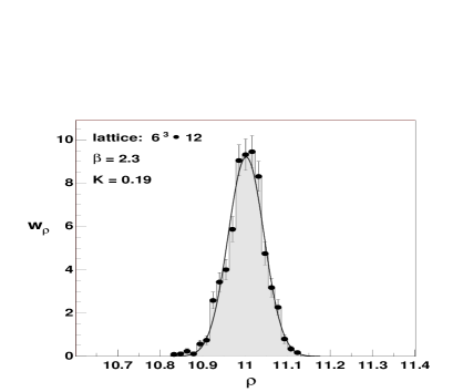
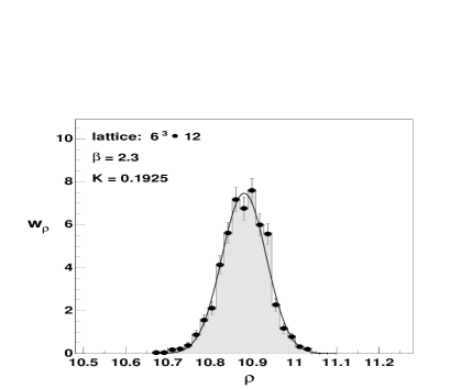
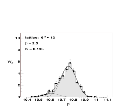
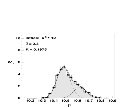
Figure 1: The probability distributions of the gaugino condensate for different hopping parameters at $\beta=2.3$ on $6^{3}\cdot 12$ lattice. The dased lines show the Gaussian components.

4 Summary and discussion

The observed dependence of the distribution of the gaugino condensate on the gaugino mass $m_{\tilde{g}}$ near $m_{\tilde{g}}=0$ is consistent with a typical behaviour characteristic of a first order phase transition between two phases (see figure 1 and table 2). Our lattice volume ($L^{3}\cdot T=6^{3}\cdot 12$) is, however, still not very large in physical units, therefore the expected two-peak structure is not yet well developed. For instance, at $K=0.1925$ we have $LM_{gg}^{0^{+}}\simeq 3.6$, with the smallest glueball mass $M_{gg}^{0^{+}}$ [13, 22]. In fact, a behaviour corresponding to a true first order phase transition can only be established in a detailed study of the volume dependence, which we postpone for future work. Therefore, the present observations are also consistent with a rapid cross-over at finite lattice spacings, approaching to a first order phase transition in the continuum limit $\beta\to\infty$. On our $6^{3}\cdot 12$ lattice for $\beta=2.3$ the phase transition (or cross-over) is at $K_{0}=0.1955\pm 0.0005$. The jump of the gaugino condensate in lattice units is $\Delta\rho\simeq 0.15$.

A rather positive aspect of our Monte Carlo simulations is the ability of the two-step multi-bosonic algorithm [9] to cope with the difficult situation at small dynamical fermion mass in the environment of metastability of phases.

In the numerical simulations we considered up to now only the unrenormalized gaugino mass and gaugino condensate. The transformation to the corresponding renormalized quantities defined in eqs. (18)-(19) will, however, not change the qualitative behaviour, because the multiplicative renormalization constants are expected to be of ${\cal O}(1)$. One has to note that in the exploited range the bare gaugino masses $m_{0\tilde{g}}$ are small compared to the lightest bound state masses. With $K_{0}=0.1955$ at $K=0.1925$ we have $m_{0\tilde{g}}/M_{gg}^{0^{+}}\simeq 0.07$. Similarly to QCD, it is expected that the mass gap in the spectrum is of the same order of magnitude as the scale parameter for the asymptotically free coupling $\Lambda$. As the preliminary results on the bound state masses show [13, 22], at $K=0.1925$ we already have an approximate degeneracy of the states which are expected to form the lowest chiral supermultiplet.

Besides the volume dependence, another interesting question is the development of the phase transition signal towards the continuum limit at $\beta=\infty$. In fact, the arguments in the introduction (at eqs. (1)-(6)) for the spontaneous chiral symmetry breaking $Z_{2N_{c}}\to Z_{2}$ refer to the continuum limit. The present numerical evidence shows that the discrete chiral symmetry breaking is manifested at non-zero lattice spacing in feasible numerical simulations and can be investigated by well established methods.

Acknowledgements: It is a pleasure to thank Gernot Münster for helpful discussions. The numerical simulations presented here have been performed on the CRAY-T3E-512 computer at HLRZ Jülich. We thank HLRZ and the staff at ZAM for their kind support.

References

- [1] D. Amati, K. Konishi, Y. Meurice, G.C. Rossi and G. Veneziano, Phys. Rep. 162 (1988) 169.
- [2] M.E. Peskin, in Proceedings of the Theoretical Advanced Study Institute in Elementary Particle Physics: Fields, Strings, and Duality, Boulder, June 1996; hep-th/9702094.
- [3] N. Seiberg and E. Witten, Nucl. Phys. B426 (1994) 19; ERRATUM ibid. B430 (1994) 485; Nucl. Phys. B431 (1994) 484.
- [4] N. Seiberg, Phys. Rev. D49 (1994) 6857; Nucl. Phys. B435 (1995) 129.
- [5] G. Veneziano, S. Yankielowicz, Phys. Lett. B113 (1982) 231.
- [6] G.R. Farrar, G. Gabadadze, M. Schwetz, Phys. Rev. D58 (1998) 015009; hep-th/9806204.
- [7] H. Nicolai, Nucl. Phys. B140 (1978) 294.
- [8] K.G. Wilson, Phys. Rev. D10 (1974) 2445; in New Phenomena in Subnuclear Physics, ed. A. Zichichi, Plenum Press, 1975, p. 69.
- [9] I. Montvay, Nucl. Phys. B466 (1996) 259.
- [10] A. Donini, M. Guagnelli, P. Hernandez, A. Vladikas, Nucl. Phys. B523 (1998) 529.
- [11] I. Montvay, Nucl. Phys. Proc. Suppl. 63 (1998) 108.
- [12] G. Curci and G. Veneziano, Nucl. Phys. B292 (1987) 555.
- [13] R. Kirchner, S. Luckmann, I. Montvay, K. Spanderen, J. Westphalen, to appear in the proceedings of the Lattice ’98 Conference, Boulder, July 1998, hep-lat/9808024.
- [14] G. t’Hooft, Nucl. Phys. B153 (1979) 141.
- [15] E. Witten, Nucl. Phys. B202 (1982) 253.
- [16] K. Spanderen, Monte Carlo simulations of SU(2) Yang-Mills theory with dynamical gluinos, PhD Thesis, University Münster, August 1998 (in German).
- [17] M. Lüscher, Nucl. Phys. B418 (1994) 637.
- [18] I. Montvay, Comput. Phys. Commun. 109 (1998) 144.
- [19] A.D. Kennedy, J. Kuti, Phys. Rev. Lett. 54 (1985) 2473.
- [20] R. Frezzotti, K. Jansen, Phys. Lett. B402 (1997) 328.
- [21] G. Koutsoumbas, I. Montvay, A. Pap, K. Spanderen, D. Talkenberger, J. Westphalen, Nucl. Phys. Proc. Suppl. 63 (1998) 727.
- [22] R. Kirchner, S. Luckmann, I. Montvay, K. Spanderen, J. Westphalen, in preparation.
- [23] N. Evans, S.D.H. Hsu, M. Schwetz, hep-th/9707260.
- [24] A. Kovner, M. Shifman, Phys. Rev. D56 (1997) 2396.