Field transformation and Monte Carlo simulations

Abstract

A new method to compute observables at many values of the parameters $\lambda$ for a model with lattice action ${\cal{S}}(\phi,\lambda)$ is described. After fixing a reference set $\lambda^{r}$ of parameters, a single simulation is carried out by using a “reference action” ${\cal{S}}(\phi^{r},\lambda^{r})$ to generate configurations of the field $\phi^{r}$. Then a suitable analytic transformation is performed from the configurations of $\phi^{r}$ to the ones corresponding to the action ${\cal{S}}(\phi,\lambda)$. Such a transformation allows to obtain the observables for values of the parameters $\lambda$ close to $\lambda^{r}$. I present studies on the reliability of the algorithm in the case of the $\phi^{4}$ model in 2 dimensions.

1 INTRODUCTION

Usually in Monte Carlo (MC) simulations observables are measured at the values of the Lagrangian parameters at which the run is carried out. However, it is often necessary to evaluate observables at many different values of the parameters, for instance, in problems requiring a fine tuning. This poses dramatic limitations to the numerical studies.

The reweighting technique [1] has long been a way out of this problem. Let us consider a single MC run performed according to a reference action ${\cal{S}}[\phi,\lambda^{r}]$ with given values $\lambda^{r}$ for the Lagrangian parameters. Field configurations are generated with probability $e^{-{\cal{S}}[\phi,\lambda^{r}]}$ and expectation values for observables are computed averaging over these configurations. Since the equilibrium distribution is known, physical quantities can be estimated for different parameters without performing a new simulation. The expectation value of an observable for the set of parameters $\lambda$ can be calculated as a reweighted average from the configurations generated by the MC simulation performed at the set $\lambda^{r}$. Moreover, the field configurations generated according to $e^{-{\cal{S}}[\phi,\lambda^{r}]}$ must be a good sampling for the distribution $e^{-{\cal{S}}[\phi,\lambda]}$. In the limit of an infinite number of configurations, $e^{-{\cal{S}}[\phi,\lambda]}$ is always correctly reconstructed but, as this is not the real case, there is a systematic distortion of the equilibrium distribution. To minimize this effect, the parameter set $\lambda$ should not differ much from the reference set $\lambda^{r}$.

Recently, an alternative technique [2] has been proposed to compute observables at various values of the couplings and masses by a single MC simulation. This method is based on a ”field transformation” from a reference field $\phi^{r}$, distributed with probability proportional to $e^{-{\cal{S}}[\phi^{r},\lambda^{r}]}$, to a field $\phi$ distributed according to $e^{-{\cal{S}}[\phi,\lambda]}$. The transformation is defined by the equation

$${\cal{D}}\phi\;e^{-{\cal{S}}[\phi,\lambda]}={\cal{D}}\phi^{r}e^{-{\cal{S}}[\phi^{r},\lambda^{r}]}$$ (1)

Thus, an importance sampling for the field $\phi^{r}$ can be transformed into an importance sampling for the field $\phi$. I will explore this technique by using a simplified version of (1). More precisely, I consider only the terms of the action depending on single sites. This simplification implies that it is necessary to reweight the data for observables with a suitable remainder action $\delta{\cal{S}}[\phi^{r},\lambda,\lambda^{r}]$. Work is in progress to take into account the full action.

Here I study how reliable is the field transformation technique compared with the reweighting method. The model I consider is the lattice $\phi^{4}$ scalar field theory in two dimensions.

2 THE CASE STUDIED: THE TWO-DIMENSIONAL $\phi^{4}$ MODEL

I consider the $2-d$ lattice scalar $\phi^{4}$ field theory with periodic boundary conditions and $L^{2}$ sites.

The lattice action is

$${\cal{S}}[\phi,\lambda]=-\frac{1}{2}\sum_{n\mu}\phi_{n}(\phi_{n+\mu}+\phi_{n-\mu})+\sum_{n}v^{\lambda}(\phi_{n})$$ (2)

where ( $\lambda\equiv(\lambda_{2},\lambda_{4})$ )

$$v^{\lambda}(\phi_{n})=\frac{1}{2}(\lambda_{2}+4)\phi_{n}^{2}+\frac{1}{4}\lambda_{4}\phi_{n}^{4}$$ (3)

The sum over $\mu$ is to be intended in the positive directions.

The expectation value for a monomial $P[\phi]=\phi_{n_{1}}\;\phi_{n_{2}}\ldots\phi_{n_{k}}$ in the field is defined to be

$$<P[\phi]>_{\lambda}\equiv\frac{1}{\cal{Z}}\int\prod_{n}d\phi_{n}\;e^{-{\cal{S}}[\phi,\lambda]}P[\phi]$$ (4)

where ${\cal{Z}}$ is the partition function.

A generic field transformation $\phi=\phi(\phi^{r})$ is defined by the jacobian matrix:

$${\cal{J}}_{nm}=\frac{\partial\phi_{n}}{\partial\phi^{r}_{m}}$$ (5)

Re-expressing the field polynomial $P[\phi]$ in terms of $\phi^{r}$, we obtain a function ${\cal{P}}[\phi^{r}]$ of the reference field. The same transformation in the measure of the functional integral yields

$$\prod_{n}d\phi_{n}\;e^{-{\cal{S}}[\phi,\lambda]}=\prod_{n}d\phi^{r}_{n}\;e^{-{\cal{S}}[\phi^{r},\lambda^{r}]+\delta{\cal{S}}[\phi^{r},\lambda,\lambda^{r}]}$$ (6)

where $\delta{\cal{S}}$, the ”remainder action”, is

$$\delta{\cal{S}}[\phi^{r},\lambda,\lambda^{r}]=-{\cal{S}}[\phi,\lambda]+{\cal{S}}[\phi^{r},\lambda^{r}]+\mbox{Tr}\;\ln{\cal{J}}$$ (7)

Now the Green function assumes the following form

$$<P[\phi]>_{\lambda}=\frac{<{\cal{P}}[\phi^{r}]\;e^{\delta{\cal{S}}[\phi^{r}]}>_{\lambda^{r}}}{<e^{\delta{\cal{S}}[\phi^{r}]}>_{\lambda^{r}}}$$ (8)

The remainder action vanishes if (1) is exactly solved, otherwise it enters as a reweighting term. The integration of (5) for a pair $\lambda\equiv(\lambda_{2},\lambda_{4})$ allows to compute ${\cal{P}}[\phi^{r}]$ and $\delta{\cal{S}}[\phi^{r},\lambda,\lambda^{r}]$ for each MC generated configuration of the reference field $\phi^{r}$. Then by averaging over the reference field configurations, one obtains the Green function $<P[\phi]>_{\lambda}$ corresponding to the Lagrangian with parameters $\lambda$.

2.1 Form of the Field Transformation

The field transformation defined by (1) is not easily integrable. Thus, a simpler case has been considered. In the simulation, I have used the following diagonal jacobian:

$${\cal{J}}_{nm}=\frac{\partial\phi_{n}}{\partial\phi^{r}_{m}}=C\delta_{nm}\;e^{v^{\lambda}(\phi_{n})-v^{\lambda^{r}}(\phi_{n}^{r})}$$ (9)

where $C$ is a constant. The solution of the previous differential equation with the condition $\phi_{n}=0$ when $\phi_{n}^{r}=0$ is

$$\int_{0}^{\phi_{n}}d\phi\;e^{-v^{\lambda}(\phi)}=C\int_{0}^{\phi_{n}^{r}}d\phi\;e^{-v^{\lambda^{r}}(\phi)}$$ (10)

The fields $\phi$ and $\phi^{r}$ are non-compact and the constant $C$ is determined requiring that $\phi_{n}\rightarrow\infty$ when $\phi_{n}^{r}\rightarrow\infty$.

With the choice (9), it follows

$$\mbox{Tr}\;\ln\;{\cal{J}}=\sum_{n}[v^{\lambda}(\phi_{n})-v^{\lambda^{r}}(\phi_{n}^{r})]$$ (11)

and consequently a non vanishing remainder action has to be used in (8) to evaluate Green functions as a ratio of reweighted averages.

2.2 Field Transformation and Reweighting

In this section I report on the tests of confidence performed for the field transformation method. These results are compared with those obtained by the reweighting technique. This analysis extends the first studies of reliability carried out for the $\phi^{4}$ scalar field theory in 4 dimensions [2]. I have examined the susceptibility and the expectation value of the action ${\cal{S}}[\phi,\lambda]$.

The MC simulation has been performed at the reference point $\lambda^{r}=(-.2,.23)$ and 66 pairs of parameters have been considered: 28 pairs had $\lambda_{2}=\lambda_{2}^{r}$ (group 1), while the remaining 38 ones had $\lambda_{4}=\lambda_{4}^{r}$ (group 2). Moreover, independent MC simulations have been carried out to check the results.

In the reference simulation 210000 uncorrelated data for the action and 40000 uncorrelated data have been collected for the susceptibility; the MC test runs have amounted to 40000 uncorrelated data.

The figures below show the results for the expectation value of the action.

Figure 1: Expectation value of the action for the group 1 pairs

Figure 2: Expectation value of the action for the group 2 pairs

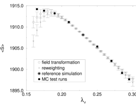
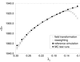
Both for the group 1 and the group 2 pairs, the reweighting technique, the field transformation method and the MC test runs agree within the error bars, except at small values of $\lambda_{2}$ and $\lambda_{4}$ where the field transformation method performs better.

The results for the susceptibility are analogous: the agreement between reweighting, field transformation and MC test runs is within one standard deviation provided that the values of $\lambda_{2}$ and $\lambda_{4}$ are not small and the critical region is not approached.

As a consequence of the choice (9) for the field transformation, the statistical error analysis is similar to that performed for the reweighting technique [3].

3 CONCLUSIONS

The field transformation method is a generalization of the reweighting technique. The simple case considered of a field transformation depending on single sites does not provide a substantial improvement respect to reweighting. Though the studies presented are preliminary, the results obtained are similar to those given by the reweighting technique. However, including the full action in the field transformation could yield a consistent improvement in the algorithm. Work is in progress in this direction. The aim is to modify the field transformation in order to eliminate the need of the weight.

References

• [1] Z. W. Salzburg et al, J. Chem. Phys. 30 (1959) 65
J. P. Valleau, D. N. Card, J. Chem. Phys. 57 (1972) 5457
A. M. Ferrenberg, R. H. Swendsen, Phys. Rev. Lett. 61 (1988) 2635; 63 (1989) 1195; Erratum 63 (1989) 1658
R. H. Swendsen, J. S. Wang, A. M. Ferrenberg, in The Monte Carlo Method in Condensed Matter Physics edited by K. Binder (Springer, Berlin, 1992).
• [2] B. Allรฉs, P. Butera, M. Della Morte, G. Marchesini, hep-lat/9807007.
• [3] A. M. Ferrenberg, D. P. Landau, R. H. Swendsen, Phys. Rev. E 51 (1995) 5092
A. M. Ferrenberg, D. P. Landau, K. Binder J. Stat. Phys. 63 (1991) 867
H. Mรผller-Krumbhaar, K. Binder, J. Stat. Phys. 8 (1973) 1
E. Munger, M. Novotny, Phys. Rev. B 43 (1991) 5773
M. E. Newman, R. G. Palmer, cond-mat/9804306