Local topological and chiral properties of QCD

Abstract

To elucidate the role played by instantons in chiral symmetry breaking, we explore their properties, in full QCD, around the critical temperature. We study in particular spatial correlations between low-lying Dirac eigenmodes and instantons. Our measurements are compared with the predictions of instanton-based models.

We have examined the local topological structure of full QCD and its impact on the physics of chiral symmetry breaking and restoration, by comparing the local topological structure obtained by improved cooling[1], with the lowest eigenmodes of the Dirac operator on the same (uncooled) lattices. We use a set of dynamical finite temperature $N_{t}=12$ (MILC[2]) lattices spanning the chiral phase transition, and have extracted the lowest 8 eigenmodes and eigenvalues of the staggered Dirac operator.

To summarize our findings, we see:

$\bullet$ agreement with the Banks-Casher relationship using the density of eigenvalues near zero (not discussed in this writeup).

$\bullet$ good correlation ($\sim$ 70% level) between the spatial structure of zero modes and instantons.

$\bullet$ some space-time asymmetry in the local topological susceptibility above $T_{c}$ (and not below), the underlying mechanism of which is under further investigation.

1. LOCAL STRUCTURE

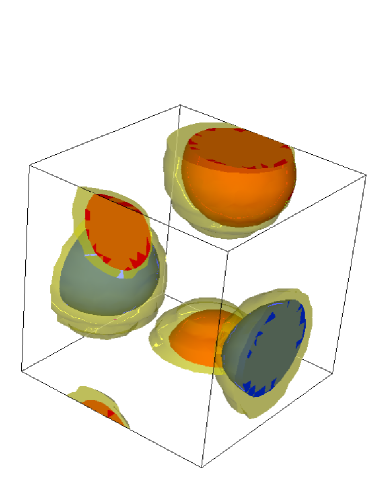
Figure 2: Isosurfaces of topological charge density $F\tilde{F}(x)$ (red[+] and blue[-]) and $\bar{\psi_{0}}(x)\psi_{0}(x)$ (yellow) using the lowest eigenmode $\psi_{0}$. Here $\bar{\psi_{0}}(x)\psi_{0}(x)$ is computed on the cooled configuration.

To illustrate the relationship between instantons and the zero modes of the Dirac operator we show in Figures 2 and 3, the topological charge density $F\tilde{F}(x)$, on a configuration obtained after 150 sweeps of improved cooling. The timeslice shown happens to contain part of an instanton and anti-instanton, and we plot isosurfaces of positive and negative values of $F\tilde{F}(x)$.

On this cooled configuration, we identify the lowest eigenmode of the Dirac operator; an isosurface of the magnitude of the eigenvector is plotted along with $F\tilde{F}(x)$, and is shown in Figure 2. We see that on this smooth configuration in which the UV fluctuations have been removed, $|\bar{\psi}\psi(x)|$ follows $F\tilde{F}(x)$ exactly, showing that on continuum like configurations, the zero mode “tracks” the topology, as expected from continuum arguments.

Next, Figure 3b compares the uncooled zero mode to the cooled topological charge; we see surprisingly good correlation, even after many (150) cooling sweeps. Cooling identifies the dominant instanton—anti-instanton (I-A) pairs and the ensemble correlation between the uncooled Dirac mode and cooled topological charge density is about 70%, after 150 sweeps of improved cooling, on configurations containing one or more I-A pairs. This validates a posteriori the improved cooling process; the topology seen by the Dirac zero mode is largely the same as that seen by the cooled topological charge.

In Figure 3a, we show isosurfaces of $\bar{\psi}\gamma_{5}\psi(x)$, which takes value $\pm 1$ for a right- or left-handed eigenmode respectively. Yellow and blue surfaces indicate right and left-handedness. We see what amounts to the chirality flip as quarks “tunnel” from an instanton to an anti-instanton.

2. ABOVE $T_{c}$

At $T\sim 1.25~{}T_{c}$, all configurations have Q=0, as $\chi\rightarrow 0$ sharply. It is very difficult to say that there are instantons and anti-instantons. After a minimal degree of smoothing ($\sim$20 cooling sweeps) a fit to non-interacting (anti)instantons or calorons does not converge. Before that, the configurations are too rough to attempt any topological identification, and we cannot really say for sure that there are instantons at all.

We can however try to characterize the fluctuations of $F\tilde{F}(x)$. In instanton liquid models[3], instanton—anti-instanton dipoles are thought to orient in the timelike direction. Inspired by this theoretical picture we examined our data in the following way[4].

We slice the lattice up into smaller sublattices, taking slabs of a given thickness $d$. While the slabs have a given thickness in direction $\mu$, they span the lattice in the other three directions. $\mu$ is chosen either along the time axis or one of the spatial axes, so that our slabs span either space or time. Within the slab we compute $\int[F\tilde{F}(x)]^{2}d^{4}x=Q^{2}_{\rm slab}$, then average over all possible slabs of thickness $d$ which are of the same orientation w.r.t. space or time.

If instantons and anti-instantons are randomly placed in an isotropic lattice, we expect that, up to a volume normalization factor, spatial and temporally oriented slabs of the same thickness $d$ should have the same value of $\langle Q^{2}\rangle_{d}$. This is what we see on the lattices below $T_{c}$.

If dipole pairs have formed in the timelike direction, we would expect $\langle Q^{2}\rangle_{d}$ to plateau for large $d$ for slabs which span the time-like direction ($\mu$ in the spatial direction). This is because we are always adding a $Q=0$ pair to the slab as we increase its thickness, and this does not increase $Q^{2}$ in the slab. For spatially spanning slabs on the other hand, the addition of charge is more or less random.

What we see above $T_{c}$, after a small amount of cooling (less than 20 sweeps), is the behavior just described: a plateau in $\langle Q^{2}\rangle_{d}$ for $d$=spacelike oriented slabs (time-spanning), and no such plateau in the corresponding $d$=timelike (space-spanning) slabs. Although it is quickly washed out by cooling, the asymmetry is quite clear and unmistakable. What is less clear is its interpretation.

Figure 1: $\langle Q^{2}\rangle$ versus volume: The lattice is sliced into sections of given volume, and $\langle Q^{2}\rangle$ is computed on these. The solid curve has time-spanning slices ($d$ in the spatial direction) and the dashed curve has space-spanning slices ($d$ is in the timelike direction). If there are dipoles in a particular direction (timelike it would appear), then $\langle Q^{2}\rangle$ should plateau when slices are taken so that they span that direction. Notes: the spatial axes have been rescaled to match the temporal dimension ($N_{t}=12$), and $Q^{2}$ is measured after 5 cooling sweeps. Below $T_{c}$, both curves are identical within statistics.

It is important to note that we see this asymmetry for quenched SU(2) as well, where it is not predicted to be by instanton liquid models.

Since obtaining this result we have generated synthetic configurations with a controlled topological charge density, and computed $\langle Q^{2}\rangle_{d}$ on these. On synthetic configurations we see:

$\bullet$ For randomly placed point charges, $q(x)=\sum_{i}\pm\delta(x-x_{i})$, there is no asymmetry. This corresponds to the data below $T_{c}$.

$\bullet$ With randomly oriented dipoles having point charges, we see a trivial asymmetry of geometric origin. There is a plateau in both space and time slices, and the ratio of the plateau values is equal to the ratio of the slab sections (i.e. 2).

$\bullet$ For randomly placed calorons, we see a reverse asymmetry which shows dependence on the radius of the caloron. By reverse asymmetry, we mean that it is the space-spanning ($d$ timelike) slabs which plateau at a lower value, the reverse of what is seen in Figure 1.

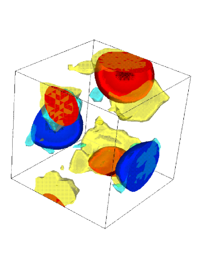
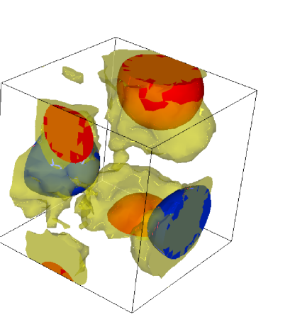
Figure 3: Isosurfaces of topological charge density $F\tilde{F}(x)$ (red[+] and blue[-]) and $\bar{\psi_{0}}(x)\psi_{0}(x)$ (yellow) using the lowest eigenmode $\psi_{0}$. Here $\bar{\psi_{0}}(x)\psi_{0}(x)$ is computed on the original uncooled configuration. Above (a), chiral components; Below (b) $|\bar{\psi_{0}}\psi_{0}(x)|$

References

- [1] Ph. de Forcrand, M. García Pérez, and I.O. Stamatescu, Nucl. Phys. B499 (1997) 409
- [2] C. Bernard et al, (MILC Collaboration) Phys.Rev. D54 (1996) 4585
- [3] T. Schäfer and E. Shuryak, Rev. Mod. Phys. 70 (1998) 323
- [4] E.-M. Ilgenfritz, E. Shuryak, Phys. Lett. B325 (1994), 263