Abstract

We discuss lattice methods to obtain the derivatives of a lattice meson mass with respect to the bare sea and valence quark masses. Applications are made to quenched and dynamical fermion configurations. We find evidence for significant differences between quenched and dynamical fermion configurations. We discuss how to relate dependence on the bare lattice parameters to more phenomenologically useful quantities.

1 Introduction

In lattice studies of QCD, the action depends on several bare parameters such as the inverse coupling $\beta$ and those controlling the quark masses. Here we distinguish the sea quarks which contribute to the vacuum and valence quarks which propagate in the vacuum but do not contribute to it. Thus there will be two possible parameters describing the quarks masses: the sea and valence hopping parameters ($\kappa_{s}$ and $\kappa_{v}$). In lattice studies, unlike experiment, it is possible to vary each of these mass parameters independently.

It is of interest to establish the dependence of quantities of physical interest, such as hadron masses, on these quark mass parameters. For instance, the valence-quark mass dependence of the meson mass controls the $J$ parameter which is related [1] to the slope of $M_{V}$ versus $M_{P}^{2}$ (where $M_{P}$ and $M_{V}$ are the pseudoscalar and vector meson masses respectively). This slope is found in lattice studies to be significantly smaller than the experimental value. It is a challenge for dynamical fermion studies on a lattice to narrow this discrepancy as the sea quark mass is reduced. Another area of current interest is the magnitude of sea quark effects on hadron masses. The dominant effect of sea quarks is just to renormalise the coupling ($\beta$) so it is valuable to have techniques to explore in fine detail the sea quark effects so that physically significant effects can be explored in dynamical fermion studies.

One direct way to achieve this is to study the theory at many different combinations of parameters. This is the conventional way to study the valence quark mass dependence and is reasonably efficient since the lattice configurations themselves do not depend on $\kappa_{v}$. For the sea quark mass, however, this is a computationally challenging endeavour since different gauge configurations must be constructed for each $\kappa_{s}$ value and then the finite differences of hadron masses between these different ensembles of configurations will be small and quite noisy.

One way to obtain estimates of derivatives by working with a lattice ensemble at one set of parameters is described in ref[2]. Here we specialise to explore a method to obtain the derivative of a hadron mass with respect to a parameter such as $\kappa_{s}$. The method is essentially to take formally the derivative of a lattice identity. This method, often called a ‘sum rule’, has been used before to obtain derivatives with respect to $\beta$ [3]. Here we use a similar approach to extract derivatives with respect to $\kappa_{s}$ and $\kappa_{v}$ - see also [4].

The derivative with respect to $\kappa_{v}$ involves a three point function of fermion fields and so cannot be obtained from propagators from one source only. Here we choose to use stochastic propagators [6] with maximal variance reduction [5] which allow the appropriate propagator combination to be evaluated.

For the derivative with respect to $\kappa_{s}$, a disconnected three point function is needed. In this case we use Z2 noise methods [7, 8] to evaluate the appropriate combination of propagators. We apply this to quenched and dynamical fermion gauge configurations and see a significant difference. We discuss the impact of these results on the sea-quark dependence of meson masses.

This study is exploratory and we discuss the computational effort needed to extract these derivatives with respect to bare quark masses. We also compare our results with those obtained by taking finite differences.

2 Quark mass dependences

The mesonic masses in lattice studies are determined by measuring two-point correlations of appropriate operators at large time separation $t$. We then wish to take the formal derivative with respect to a parameter representing the quark mass. This will give the required sum rules for the derivative of the lattice hadron mass with respect to the quark mass parameter.

Consider an action density

$$S=S_{f}+\beta S_{g}=\sum_{1}^{N_{f}}\bar{\psi}{\cal M}\psi+\beta S_{g}$$ (1)

where, for the Wilson-Dirac discretisation of fermions,

$${\cal M}=m+D$$ (2)

where the quark mass parameter $m\equiv 1/\kappa$, with $\kappa$ the conventional hopping parameter, so in terms of the bare quark mass $m_{b}$ in the naive continuum limit $m=8+2am_{b}$. The term $D$ contains the Wilson nearest neighbour gauge link terms as well as the SW-clover terms with coefficient $C_{SW}$. The hadronic correlation is then given by

$$C(t)={1\over Z}\int H(0)H^{{\dagger}}(t)e^{S}$$ (3)

Here for mesons $H$ will be of the form $\bar{\psi}\Gamma\psi$ and in this work we will concentrate on the case of flavour non-singlet mesons so that the hairpin diagrams will not be needed. Then the fermionic degrees of freedom are integrated out giving a factor of the inverse of the fermion matrix ($G={\cal M}^{-1}$) for each pairing:

$$C(t)=\langle 0|\left(G(0,t)\Gamma G(t,0)\Gamma\right)|0\rangle$$ (4)

At large $t$, this correlation will be dominated by the ground state meson with the quantum numbers created by $H$:

$$C(t)=c_{0}^{2}e^{-M_{0}t}+\dots$$ (5)

This sketch of the formalism allows us to explore taking the derivative with respect to the quark mass parameter $m$ (actually the inverse hopping parameter) on each side of the above expressions for $C(t)$. This derivative is to be taken at fixed $\beta$. Then, since formally the only $m$-dependence is in the exponent, the derivative brings down a factor of $N_{f}\bar{\psi}\psi$.

$${dC(t)\over dm}={1\over Z}\int H(0)H^{{\dagger}}(t)N_{f}\bar{\psi}\psi e^{S}-C(t){1\over Z}\int N_{f}\bar{\psi}\psi e^{S}$$ (6)

where the second term comes from the $m$-dependence implicit in $Z$. On integrating out the six fermions, this will give two diagrams, connected and disconnected (actually only the connected part of the disconnected diagram will contribute as discussed below). Thus, summing explicitly over the insertion at $t_{1}$, we have

$${dC(t)\over dm}=\sum_{t_{1}}\left(-C_{3}(t_{1},t)+N_{f}D_{3}(t_{1},t)\right)$$ (7)

Figure 1:

The diagrams corresponding to $C_{3}$ and $D_{3}$.

Where for the connected diagram there will be terms from the insertion on either quark line:

$$C_{3}(t_{1},t)=\langle 0|\left(G(0,t_{1})G(t_{1},t)\Gamma G(t,0)\Gamma\right)+\left(G(0,t)\Gamma G(t,t_{1})G(t_{1},0)\Gamma\right)|0\rangle$$ (8)

while the disconnected diagram is, for each flavour of quark in the loop,

$$D_{3}(t_{1},t)=\langle 0|\left(G(0,t)\Gamma G(t,0)\Gamma\right)\left(G(t_{1},t_{1})\right)|0\rangle-\langle 0|\left(G(0,t)\Gamma G(t,0)\Gamma\right)|0\rangle\langle 0|\left(G(t_{1},t_{1})\right)|0\rangle$$ (9)

where curved brackets imply a trace over colour, spin and space coordinates.

In the quenched approximation, only the connected diagram contributes. This can be seen another way since ${\cal M}G=1$ implies ${\cal M}dG/dm+d{\cal M}/dm\,G=0$ and since $d{\cal M}/dm=1$ by definition, then $dG/dm=-{\cal M}^{-1}G=-GG$. Thus either fermion propagator in the mesonic correlator can be ‘opened’ by an insertion.

For dynamical fermions, both types of diagram contribute but one can see that the connected diagram corresponds to varying the valence quark mass while the disconnected diagram corresponds to varying the sea quark mass.

The two point hadronic correlation can be expressed in terms of a sum over intermediate states of masses $M_{i}$

$$C(t)=\sum_{i}c_{i}^{2}e^{-M_{i}t}$$ (10)

The leading term in the derivative at large $t$ can be then be evaluated

$${dC(t)\over dm}=-t{dM_{0}\over dm}c_{0}^{2}\,e^{-M_{0}t}+{dc_{0}^{2}\over dm}e^{-M_{0}t}+\dots$$ (11)

and it thus behaves as $te^{-M_{0}t}$ where $M_{0}$ is the ground state meson mass.

We now extract the contribution from the right hand side which has this same behaviour. For both $C_{3}$ and $D_{3}$, the insertion is summed over all space and time. Then the leading term arises when the lightest allowed meson propagates and when $0<t_{1}<t$. This will produce terms which are linear in $t$ which arise from the $t$ possible insertions (at $t_{1}$) between the creation and destruction of the meson. Then evaluating this ground state meson contribution, for the connected diagram, gives

$$\sum_{t_{1}}C_{3}(t_{1},t)=c_{0}^{2}\,t\left(X^{(1)}+X^{(2)}\right)e^{-M_{0}t}=t\,\left(X^{(1)}+X^{(2)}\right)C(t)$$ (12)

where the suffix refers to the insertion on quark propagator 1 or 2 and $X$ is the matrix element of the $\bar{\psi}\psi$ insertion between ground state hadrons. A similar expression applies for the disconnected case.

Equating the coefficients of the terms behaving as $te^{-M_{0}t}$ on each side of the identity, then gives the exact result that

$${dM_{0}\over dm_{v}}=X^{(1)}+X^{(2)}$$ (13)

where the matrix element sum can be obtained by extracting the ground state contribution to $C_{3}/C$. In principle this can be obtained by taking the insertion in $C_{3}$ such that $0<t_{1}<t$ and both $t_{1}$ and $t-t_{1}$ are large so that the ground state contributes. So we can write

$${dM_{0}\over dm_{v}}=\lim_{t_{1},(t-t_{1})\to\infty}{C_{3}(t_{1},t)\over C(t)}$$ (14)

This sum rule relates the derivative to an expression that can be evaluated from lattice configurations at only one set of parameters. It is an exact identity. If there is a dependence of the lattice meson mass $M_{0}$ on the finite spatial size $L$ of the lattice, the derivative should be taken at fixed number of lattice spacings, not at fixed physical size. These considerations are very similar to those used in the lattice sum rules derived by taking formal derivatives with respect to $\beta$ [3].

For the disconnected diagram, the equivalent expression is

$${dM_{0}\over dm_{s}}=-N_{f}\lim_{t_{1},(t-t_{1})\to\infty}{D_{3}(t_{1},t)\over C(t)}$$ (15)

In order to evaluate these expressions on a lattice, it is useful to consider efficient ways in which excited state contributions can be eliminated, since the formal limits of large $t$ will have big noise to signal. Here we consider the connected correlation $C_{3}$ and use a complete set of hadron states of mass $M_{i}$ in the intermediate intervals of time extent $t_{1}$ and $t_{2}=t-t_{1}$.

In practice, we will be using more than one operator to create and destroy the hadronic state. This allows an optimal combination of these operators to be formed that minimises the excited state contribution. Then the two-body correlation between operators $a$ at $t=0$ and $b$ at $t$ will be given by

$$C^{(ab)}(t)=\sum_{i}c^{(a)}_{i}e^{-M_{i}t}c^{(b)}_{i}$$ (16)

$$C_{3}^{(ab)}(t_{1},t_{2})=\sum_{i,j}c^{(a)}_{i}e^{-M_{i}t_{1}}x_{ij}e^{-M_{j}t_{2}}c^{(b)}_{j}$$ (17)

where $x_{00}$ is the required quantity ($X^{(1)}+X^{(2)})$ - the matrix element appropriate to the ground state meson of mass $M_{0}$. We might expect $x_{11}$ to be similar in sign and magnitude to $x_{00}$ if the quark mass dependence of the excited state is comparable to that of the ground state and thus excited state contributions would cancel in the ratio $C_{3}/C$. This is incorrect, since the off-diagonal terms ($x_{01}$) will dominate the excited state contributions to $C_{3}$ since the excited state only propagates for the shorter interval $t_{1}$ (or $t_{2}$). One way to extract $x_{00}$ is to make a fit to the three point data with both $t_{1}>t_{\rm min}$ and $t_{2}>t_{\rm min}$, keeping the coefficients and masses ($c^{(a)}_{i}$ and $M_{i}$) fixed from the fit to the two-point function data with $t>t_{\rm min}$. This can be compared with the more direct approach of looking for a plateau in $C_{3}(t_{1},t_{2})/C(t)$ as $t_{1}$ and $t_{2}$ are increased (with $t=t_{1}+t_{2}$).

When two (or more) different types of hadronic creation operators are used, a variational method is an effective way to determine the ground state contribution to $C$ and hence to extract the ground state contribution to $C_{3}$. Alternatively, if a two state fit to the two-body correlation between two operators at each end is made, then from the coefficients, it follows that a combination of operators $c^{(2)}_{1}H_{1}-c^{(1)}_{1}H_{2}$ will remove the contribution of the excited state in the approximation that only two states contribute to the correlations. Then we can use this combination to evaluate the ground state component of $C_{3}/C$, using

$${c_{1}^{(2)}c_{1}^{(2)}C_{3}^{(11)}-2c_{1}^{(2)}c_{1}^{(1)}C_{3}^{(12)}+c_{1}^{(1)}c_{1}^{(1)}C_{3}^{(22)}\over c_{1}^{(2)}c_{1}^{(2)}C^{(11)}-2c_{1}^{(2)}c_{1}^{(1)}C^{(12)}+c_{1}^{(1)}c_{1}^{(1)}C^{(22)}}$$ (18)

A similar analysis holds equivalently for the extraction of the ground state contribution $d_{00}$ to $D_{3}$.

When $t\approx T/2$, the contributions from propagation around the time boundary of the lattice may be significant. For $C_{3}$ there will be no such ‘round the back’ term because the insertion is made explicitly, while for $D_{3}$ the connected matrix element involved will cancel for the round the back term. In contrast the two-body correlator $C$ will be a sum of two terms. Illustrating this for the ground state component for one type of operator, we have:

$$C=c_{0}^{2}e^{-M_{0}t}+c_{0}^{2}e^{-M_{0}(T-t)}$$ (19)

$$C_{3}=c_{0}^{2}e^{-M_{0}t}x_{00}$$ (20)

Hence

$$C_{3}/C=x_{00}{1\over 1+e^{M_{0}(T-2t)}}$$ (21)

This formalism can be used to correct for the different $t$-dependences when looking for a plateau in $C_{3}/C$ and in $D_{3}/C$ as $t$ increases.

We now discuss efficient methods to evaluate these correlators on a lattice.

3 Valence quark mass dependence

As a first application, we consider the dependence of the hadron mass on the valence quarks. For this a three point function needs to be evaluated - see fig. 1a. Thus conventional quark propagators from one source are inadequate for this task. One feasible way forward is to use a stochastic inversion method which allows the evaluation of quark propagators from any site to any other site. Although the stochastic method is not more efficient than the conventional inversion from one source for mesons made of light quarks [5], it does allow the flexibility to evaluate three point correlations readily. For this reason it allows an exploratory study of this area.

Stochastic propagators [5, 6] are one technique to invert the fermionic matrix for the light quarks. They can be used in place of light quark propagators calculated with the usual deterministic algorithm. The stochastic inversion is based on the relation:

$$G_{ij}={\cal M}_{ij}^{-1}=\frac{1}{Z}\int{\cal D}\phi\;({\cal M}_{jk}\phi_{k})^{\ast}\phi_{i}\;\exp\left(-\phi_{i}^{\ast}({\cal M}^{\dagger}{\cal M})_{ij}\phi_{j}\right)$$ (22)

where, in our case, ${\cal M}$ is the improved Wilson-Dirac fermionic operator and the indices $i,j,k$ represent simultaneously the space-time coordinates, the spinor and colour indices. For every gauge configuration, an ensemble of independent fields $\phi_{i}$ (we use 24 following [5]) is generated with gaussian probability:

$$P[\phi]=\frac{1}{Z}\exp\left(-\phi_{i}^{\ast}({\cal M}^{\dagger}{\cal M})_{ij}\phi_{j}\right)$$ (23)

All light propagators are computed as averages over the pseudo-fermionic samples:

$$G_{ij}=\left\{\begin{array}[]{l}\langle({\cal M}\phi)_{j}^{\ast}\phi_{i}\rangle\\ \mathrm{or}\\ \gamma_{5}\langle\phi_{j}^{\ast}({\cal M}\phi)_{i}\rangle\gamma_{5}\end{array}\right.$$ (24)

where the two expressions are related by $G_{ij}=\gamma_{5}G_{ji}^{\dagger}\gamma_{5}$. Moreover, the maximal variance reduction method is applied in order to minimise the statistical noise [5]. The maximal variance reduction method involves dividing the lattice into two boxes ($0<t<T/2$ and $T/2<t<T$) and solving the equation of motion numerically within each box, keeping the pseudo-fermion field $\phi$ on the boundary fixed. According to the maximal reduction method, the fields which enter the correlation functions must be either the original fields $\phi$ or solutions of the equation of motion in disconnected regions. The stochastic propagator is therefore defined from each point in one box to every point in the other box or on the boundary. For this reason, when computing the three-point correlation function,

$$\sum_{x,y,z}\langle 0|H(t_{1},x){\cal O}(t_{0},y)H^{\dagger}(t_{2},z)|0\rangle$$ (25)

the operator ${\mathcal{O}}$ (which is $\bar{\psi}\psi$) is forced to be on the boundary ($t_{0}=0$ or $T/2$) and the other two operators must be in different boxes, while the spatial coordinates are not constrained. If $j$ is a point of the boundary, not all the terms in $({\cal M}\phi)_{j}$ lie on the boundary because the operator ${\cal M}$ involves first neighbours in all directions. Hence, whenever a propagator $G_{ij}$ is needed with one of the points on the boundary, we use whichever of the two expressions in Eq. 24 has ${\cal M}\phi$ computed away from the boundary. This implies that we are restricted to $t\geq 2$.

The numerical analysis used 24 stochastic samples on each of 20 quenched gauge configurations, generated [5] on a $12^{3}\times 24$ lattice at $\beta=5.7$, corresponding to $a^{-1}=0.91$ GeV. With improved clover coefficient $C_{SW}=1.57$, we use two values of $\kappa$: $\kappa_{1}=0.14077$ and $\kappa_{2}=0.13843$. The lighter value $\kappa_{1}$ corresponds to a bare mass of the light quark around the strange mass. The chiral limit corresponds to $\kappa_{c}=0.14351$ [9]. Error estimates come from bootstrap over the gauge configurations. We also made an exploratory study of some dynamical fermion configurations, as will be discussed later.

In smearing the hadronic interpolating operators, spatial fuzzed links are used. Following the prescription in [5, 10], to which the interested reader should refer for details, the fuzzed links are defined iteratively as:

$$U_{\mathrm{new}}={\mathcal{P}}\left(fU_{\mathrm{old}}+\sum_{i=1}^{4}U_{\mathrm{bend},i}\right)$$ (26)

where ${\mathcal{P}}$ is a projector over $SU(3)$, and $U_{\mathrm{bend},i}$ are the staples attached to the link in the spatial directions. Five iterations of fuzzing with $f=2.5$ are used and then the fuzzed links are combined to straight paths of length three. The fuzzed fermionic fields are defined following [10].

We employed two types of hadronic operator for the correlations - local and fuzzed - yielding a $2\times 2$ matrix. From this we use a variational approach to extract the linear combination of operators which maximises the ground state contribution - as described above. Since we are able to get good two state fits to the two-body correlations for the pseudoscalar meson for $t\geq 3$, this variational linear combination was determined using $t$-values 3 and 4. In order to maximise the ground state contribution relative to excited states, we evaluated the three point diagram $C_{3}(t_{1},t_{2})$ using values of $t_{1}$ and $t_{2}$ near to $t/2$ where $t=t_{1}+t_{2}$. The ground state improved ratio of $C_{3}(t_{1},t_{2}/C(t)$ is plotted in fig. 2. The extraction of the ground state should be good if $t_{1},t_{2}\geq 3$. For odd values of $t$ there are higher statistics (from the 3,4 and 4,3 partitions of t=7 for instance). Thus we expect $t=7$ to be the best determined value and this is given in table 1. Consistency at higher $t$-values confirms that the ground state extraction is correct.

Table 1: Connected loop correlations.

$\kappa_{v}$	$M_{P}$	$dM_{P}/dm_{v}$	$M_{V}$	$dM_{V}/dm_{v}$	$n_{\rm gauge}$
0.14077	0.529(2)	1.97(27)	0.815(5)	1.9(9)	20
0.13843	0.736(2)	1.56(22)	0.938(3)	0.3(4)	20
0.1395	0.558(8)	1.3(3)	0.786(9)	0.2(1.1)	5

Figure 2: The connected correlation $C_{3}/C$ versus time $t=t_{1}+t_{2}$ in lattice units. The data are for the variational combination that reduces the excited state contribution and are from quenched lattices with $\kappa=0.14077$ with $|t_{1}-t_{2}|<2$. We expect the ground state contribution to be dominant when $t_{1}>2$ and $t_{2}>2$, that is for $t\geq 6$.

For the pseudoscalar meson, we expect that $M_{P}^{2}$ is approximately linear in $m_{v}$. Thus $dM_{p}/dm_{v}$ should decrease like $1/M_{P}$ which is indeed consistent with the results shown in table 1. From the high statistics spectroscopy at these two hopping parameters [9], one can evaluate the finite difference obtaining $dM_{P}^{2}/dm_{v}=2.18(4)$ which agrees very well with the values determined from the sum rules of $2M_{P}dM_{P}/dm_{v}=2.08(29)$ and 2.30(32) at $\kappa_{v}=0.14077$ and 0.13843 respectively.

For the vector meson, the expectation is that $M_{V}$ is approximately linear in $m_{v}$. The finite difference [9] gives $dM_{V}/dm_{v}=1.02(7)$. The sum rule determination with our current statistics is too noisy at $t=7$ to give an accurate value. For the heavier quark mass ($\kappa_{v}=0.13843$) a good two-state fit to the two point correlation data can be made for $t\geq 2$. This allows us to use $t=4$ and 5 for the $C_{3}/C$ ratio and we obtain 0.90(18) and 0.93(26) respectively, in excellent agreement with the expected value. At the lighter quark mass, we need $t\geq 3$ for a two-state fit so the poor result remains. This is a disappointment, since from the values of $dM_{V}/dm_{v}$ and $dM_{P}/dm_{v}$, one can evaluate the $J$ parameter (which is the physical quantity, defined in the continuum limit as $M_{V}dM_{V}/dM_{P}^{2}$ at $M_{V}/M_{P}=1.8$) at a quark mass corresponding to $m_{v}$. Thus $J$ can be determined at the lightest quark mass directly, rather than as a difference between two quark masses. This $J$ parameter is a useful indicator [1] of the distance between quenched QCD (with $J\approx 0.37$) and experiment (with $J=0.48(2))$. Hence a quick and accurate method to determine $J$ would be useful to calibrate dynamical fermion studies.

We also evaluated the same quantities for dynamical fermion configurations [11] at $\beta=5.2$ with two flavours of sea quarks at $\kappa_{s}=0.1395$ on a $12^{3}24$ lattice using a SW-clover improved action with $C_{SW}=1.76$. The correlation was evaluated with $\kappa_{v}=\kappa_{s}$. In this case the higher statistics determination of the masses [11] allows the derivative at fixed $\kappa_{s}$ to be evaluated, giving $dM_{P}/dm_{v}=2.2(4)$ from the finite difference between $\kappa_{v}$ of 0.1395 and 0.1390. Our analysis is from only 5 gauge configurations and so the error may be underestimated because of the small sample size. For the pseudoscalar, we find acceptable two state fits for $t\geq 2$ (the hadronic operators are local and fuzzed with straight paths of 2 links) and so we may use the variational method from $t$ of 2 to 3 to determine the ground state couplings. This yields a value at t=4 and 5 of $C_{3}/C$ of 1.4(4) and 1.5(3), respectively. This is consistent with the value in table 1 and with the finite difference value within errors. The vector meson case is too noisy to be of any use. The main conclusion is that the ratio of correlations $C_{3}/C$ is very similar in the dynamical configurations to the quenched case. This is not really surprising since the sea quark masses used in the dynamical quark study are fairly large - larger than the strange quark mass.

4 Sea quark mass dependence

The disconnected diagram (see fig. 1b) involves measuring two gauge invariant contributions: the two-point hadronic correlator $C$ and the loop contribution corresponding to ${\rm Trace}{\cal M}^{-1}$ where the trace is a sum over colour, spin and spatial coordinates at a given time $t_{0}$. This needs the propagator from each site on a time slice to a sink corresponding to the same site. There is an efficient way to evaluate this making use of Z2 stochastic sources [7, 8]. Here we propose a variant of this method which is appropriate for our current study. This method also gives the two point correlator $C(t_{1},t_{2})$ for pseudoscalar mesons and vector mesons from any time $t_{1}$ to any other time $t_{2}$. Then combined with the loop contribution at $t_{0}$, we have the ingredients needed to evaluate the required connected part $D_{3}$ of the disconnected correlation.

Details of the Z2 method used are given in the Appendix. In this exploratory study on $12^{3}24$ lattices, we use local operators to create the pseudoscalar and vector mesons. We have used rather generous values of the number of Z2 samples per time slice (namely between 16 and 32 for each of the two related types of source used). This amounts to 768 or more inversions (equivalent to 64 conventional propagator inversions from 12 colour spin sources) per gauge configuration. Because of the decreased number of iterations of the inversion algorithm in our case, the time used is equivalent to about 30 conventional propagator determinations per gauge configuration. This is a substantial computational challenge, but it does provide a significant resource: the loop contributions at each $t$ and the pseudoscalar and vector correlators from any $t_{1}$ to any $t_{2}$. Because of our choice of number of Z2 samples, we have negligible errors coming from the Z2 noise for the value of ${\rm Trace}{\cal M}^{-1}$ from each time-slice and for the pseudoscalar correlator from $t_{1}$ to $t_{2}$. For the vector meson correlator, the error from the Z2 method is in some cases comparable to the intrinsic variation and we correct for this in derived quantities by increasing our errors appropriately where necessary. Indeed, in retrospect, it would have been more efficient for the present study to use less Z2 samples and to explore more gauge configurations. Our approach, however, was that so much computational effort has gone into the production of the dynamical fermion configurations that the large number of inversions used in measurement are in effect a relatively small extra overhead.

We evaluated these quantities for dynamical fermion configurations [11] at $\beta=5.2$ with two flavours of sea quarks at $\kappa_{s}=0.1390,\ 0.1395$ and 0.1398 on a $12^{3}24$ lattice using a SW-clover improved action with $C_{SW}=1.76$. In our evaluations we restrict ourselves to the case where the propagating quarks have the sea-quark mass, i.e. $\kappa_{v}=\kappa_{s}$. The number of gauge configurations used and number of Z2 samples $n_{Z}$ are given in table 2. We also quote, for completeness, the pseudoscalar and vector meson masses and the $R_{0}$ values obtained from higher statistics by conventional methods [9, 12, 11].

It is possible to measure the disconnected diagram in quenched gauge configurations as well as in dynamical fermion configurations. We use the same gauge configurations as discussed in the previous section. For the quenched case, we include a factor of $N_{f}=2$ explicitly to facilitate comparison with the dynamical fermion configurations that have $N_{f}=2$.

As discussed previously, the disconnected 3-point correlation $D_{3}(t_{1},t_{2})$ can be fitted to obtain the matrix element $d_{00}$ that gives us $dM/dm_{s}$. Because we only have data on the correlations from local hadronic operators in this study, we choose to make use of the results of conventional studies of the 2-point correlators from both local and non-local (smeared or fuzzed) operators from larger samples of configurations [9, 11] to determine the couplings $c_{i}$ of the ground state and excited state mesons to our operators. We find that adequate two-state fits can be made to these 2-point correlations for $t>2$. Then keeping the masses and coefficients $c_{i}$ fixed, we can fit all the 3-point data with $t_{1}>2$ and $t_{2}>2$. Some typical fits are shown in fig. 3. The fit results are shown in table 2: the upper two lines are from quenched configurations while the lower three lines are with dynamical fermions.

Table 2: Disconnected loop correlations.

$\kappa$	$M_{P}$	$dM_{P}/dm_{s}$	$M_{V}$	$dM_{V}/dm_{s}$	$R_{0}$	$n_{\rm gauge}$	$n_{Z}$
0.14077	0.529(2)	1.18(26)	0.815(5)	1.6(5)	2.92(1)	20	$16\times 2$
0.13843	0.736(2)	0.86(15)	0.938(3)	1.0(2)	2.92(1)	20	$16\times 2$
0.1398	0.476(14)	3.0(5)	0.706(16)	2.7(6)	3.65(4)	20	$32\times 2$
0.1395	0.558(8)	3.1(6)	0.786(9)	3.0(7)	3.44(6)	20	$32\times 2$
0.1390	0.707(5)	1.9(4)	0.901(10)	1.8(3)	3.05(7)	24	$20\times 2$

Figure 3: The disconnected correlation $-N_{f}D_{3}/C$ with $N_{f}=2$ versus time $t=t_{1}+t_{2}$ in lattice units. The upper data are from dynamical fermions with $\kappa_{\rm sea}=0.139$, while the lower data from quenched lattices with $\kappa=0.13843$. The curves show the two-state fits to these data with $|t_{1}-t_{2}|=0$ or 1 as described in the text. The additional points (crosses and octagons) have $|t_{1}-t_{2}|=2$ or 3 and are fitted by the dotted curve.

The sign of the effect implies that the loop (${\cal T}={\rm Trace}{\cal M}^{-1}$) is anti-correlated with the pion two-point correlation $C$ which straddles it in time on a lattice. This anticorrelation is large with, for example,

$$\langle\delta C\ \delta{\cal T}\rangle/(\langle(\delta C)^{2}\rangle\ \langle(\delta{\cal T})^{2}\rangle)^{1/2}\approx-0.5$$ (27)

at $t=6$ for both the dynamical fermion and quenched cases.

This anti-correlation is seen to be very similar for pseudoscalar and vector mesons. One qualitative argument for the sign of the correlation is that an upward fluctuation of $C$ corresponds to configurations in which quarks propagate easily over large distances whereas an upward fluctuation of the loop (${\cal T}$) comes from configurations in which quarks do not propagate easily - and so have a bigger amplitude at the origin. In terms of our identities which relate this disconnected correlation to the derivatives $dM/dm_{s}$, we see that the main effect comes from the dependence of the lattice spacing $a$ on $m_{s}$ at fixed $\beta$. It is well known that $a$ decreases as the sea-quark mass decreases: indeed this is why the $\beta$ value used in dynamical simulations is smaller than that used in quenched. The UKQCD study [11] of the dynamical fermion configurations we are using finds $d\,\log a/dm_{s}\approx-4$ - as shown in fig. 4. Furthermore the slope appears larger at smaller sea quark mass - in line with what we find in table 2.

Figure 4: The lattice evaluation of $R_{0}$ for dynamical fermion configurations with sea quarks of hopping parameter $\kappa$ from ref[11]. We define $m_{s}\equiv 1/\kappa$.

We also measure the same disconnected correlation in quenched configurations. The results are qualitatively similar to those from dynamical fermion configurations. This implies that one can explore the sea-quark dependence of meson masses using quenched configurations. This appears a striking advance - one can get at essential information concerning sea-quarks without the heavy computational overhead of dynamical fermion simulations. However, it is widely appreciated that most lattice observables are insensitive to the presence of sea quarks if the lattice spacing and $M_{P}/M_{V}$ ratio are lined up. Hence, once one has expressed the quantity of interest as a vacuum expectation value, it may be evaluated using quenched configurations. We now explore this in a little more detail.

For the heavier quenched ($\kappa=0.13843$) and dynamical ($\kappa=0.1390$) cases, the lattice spacings (taken from $R_{0}\approx 3$) and the $M_{P}/M_{V}$ ratio (at 0.78) are very similar. Thus we may directly compare the $dM/dm_{s}$ values obtained. From table 2, we see that $dM/dm_{s}$ has significantly smaller values (by two standard deviations) in quenched than in dynamical fermion configurations. This conclusion is reinforced by the presentation of the fits to these data shown in fig. 3. These data suggest that this observable is indeed capable of distinguishing between configurations with different sea quark structure. One note of caution is that since the lattice spacing is rather coarse, the different finite lattice spacing effects in quenched and dynamical simulations may be partly responsible for this observed difference.

This ability to distinguish quantitatively between quenched and dynamical gauge configurations is important - in most cases previously studied, no such discrimination was detectable. That the observable currently under study allows this discrimination is not entirely unexpected since the dynamical fermion configurations are weighted by ${\rm det}({\cal M})$ which is closely related to ${\rm Trace}{\cal M}^{-1}$ which is a component of the disconnected correlator.

For dynamical fermions it is possible to evaluate by conventional methods the hadronic mass differences as the sea quark mass is varied and so obtain an estimate of the derivative which can be compared with our results. For the pseudoscalar meson, finite difference determinations [11] at fixed valence quark mass of $\kappa_{v}=0.1390$ give $dM_{P}/dm_{s}=3.1(3)$ and of $\kappa_{v}=0.1395$ give $dM_{P}/dm_{s}=4.3(4)$. Both of these finite difference estimates are somewhat larger than the derivatives determined above. The situation is the same for the vector meson mass derivatives where the finite difference determinations give 3.4(5) and 4.0(1.2) at a fixed valence mass of 0.139 and 0.1395, respectively.

The two different approaches to determining these sea-quark mass derivatives used different gauge ensembles (propagators from the origin from about 100 gauge configurations for ref[11], compared to propagators from all sites on about 20 gauge configurations here) and the differences are only at the two standard deviation level. At present the quoted statistical errors from the derivative method we use are comparable to those from finite differences of masses. Using the full set of gauge configurations available, our derivative method would give the more accurate determination of the sea quark dependence of the meson masses.

5 Discussion

There are several issues of interest in determining the dependence of hadron masses on the quark masses. Here we are not concerned with the problem of defining precisely the quark masses. Rather we discuss the dependence of the meson masses as the sea quark mass is reduced to look for explicit signs of different physics as the quark loops become more important in the vacuum. One of the complicating features in the lattice approach is that changing the sea-quark mass parameter has several consequences - among them that the lattice spacing is changed.

As an illustration, since the lattice spacing $a$ depends on the sea quark parameter $m_{s}$, let us consider the dimensionless ratio $M_{V}/M_{P}$. Then

$${d\over dm_{s}}\ln({M_{V}\over M_{P}})={1\over M_{V}}{dM_{V}\over dm_{s}}-{1\over M_{P}}{dM_{P}\over dm_{s}}$$ (28)

can be evaluated. Since we find $dM_{P}/dm_{s}\approx dM_{V}/dm_{s}$, this gives a negative result which implies that the $M_{V}/M_{P}$ ratio increases as the sea quark mass is decreased. This change in sea-quark mass parameter is at a constant $\kappa_{v}$, however, which is not necessarily what is required.

To clarify this discussion, it must be remembered that the bare parameters $(\beta,\kappa_{v},\kappa_{s})$ which occur in the lattice formalism are not simply related to the more physical parameters $a$ and the sea and valence quark masses which we denote here as $q_{v}$ and $q_{s}$. One example of this intricate relationship is that as $\kappa_{s}$ is increased (i.e. towards $\kappa_{c}$ so that the sea quarks are lighter) then $a$ becomes smaller (this can be seen from the observation that $\beta$ needs to be reduced for dynamical fermions to keep $a$ approximately the same). Furthermore, this change of $\kappa_{s}$ is also likely to result in a different value of $\kappa_{c}$ (here defined as the value which gives a massless pion on varying $\kappa_{v}$ at that sea quark mass) and hence the relationship of $\kappa_{v}$ with $q_{v}$ will be modified too.

Thus one needs to set up a prescription to determine appropriate values of the lattice parameters. One proposal is to identify physical quantities which should not depend on all of the physical parameters. Thus we can choose to use $r_{0}$ (defined via the static potential at moderate separations) to determine the lattice spacing $a$, assuming it to be independent of the quark masses. This would not have been true if the string tension were to have been used to set the scale since the string breaking at large separation will be strongly affected by the sea quark mass.

For the quark mass dependence, we are considering a world where the valence quark mass $q_{v}$ can be varied independently of the sea quark mass $q_{s}$. This is not so far from experiment if one regards the $u,d$ quarks as sea quarks and the strange quark as a valence quark whose contribution to the sea is relatively small.

To isolate the quark mass dependence, we choose to make use of a very conspicuous experimental fact: the vector mesons are ‘magically mixed’ with the $\phi$ meson being almost pure $\bar{s}s$ while the $\rho$ and $\omega$ are almost degenerate and composed of $u,d$ quarks. Furthermore the $\phi$ has much reduced decay matrix elements to final states containing only $u,d$ quarks. This is the OZI rule: disconnected quark diagrams are suppressed. All of this phenomenology suggests that the vector meson nonet is well described by the naive quark model: it does not contain significant sea quark contributions to the masses. Thus we choose to define the sea quark mass $q_{s}$ such that the vector meson masses are independent of it. For other mesons, especially the pseudoscalar mesons, we do expect some dependence of the masses explicitly on the sea-quark mass $q_{s}$ and we shall try to estimate it.

One way to proceed is to remove the explicit $a$-dependence of the lattice masses by forming the product with $R_{0}$. Then $R_{0}M_{P}$ will be equal to the continuum product $r_{0}m_{P}$ up to lattice artefact corrections which are of order $a$ for the Wilson fermion discretisation but the clover-improvement scheme we use should reduce these lattice artefact corrections to being dominantly of order $a^{2}$. For ease of notation we define $P_{s}=d(R_{0}M_{P})/dm_{s}$ etc. Here we assume, as discussed above, that $R_{0}$ is independent of $m_{v}$ and that it does depend on $m_{s}$ through the dependence of $a$ on $m_{s}$. This sea quark mass dependence of $R_{0}$ can be extracted by explicitly evaluating $R_{0}$ at a range of $m_{s}$ values [11], as illustrated in fig. 4, giving

$${1\over R_{0}}{dR_{0}\over dm_{s}}=-4.7(1.8)\ ;-4.0(2.0)$$ (29)

where differences are taken from $\kappa_{s}$ of 0.1390 to 0.1395 and then 0.1395 to 0.1398 respectively. These values can then be used to obtain

$${1\over R_{0}M_{P}}P_{s}={1\over R_{0}M_{P}}{d(R_{0}M_{P})\over dm_{s}}={1\over R_{0}}{dR_{0}\over dm_{s}}+{1\over M_{P}}{dM_{P}\over dm_{s}}$$ (30)

where a substantial cancellation occurs between the latter two terms. Thus we find that the resulting errors are sufficiently large that even the sign of $P_{s}$ is not well determined. However, the sign of $P_{s}$ does not necessarily have any direct physical meaning as we now discuss.

Assuming one had accurate values, we now discuss how to interpret them. The situation is illustrated on a plot of $P\equiv R_{0}M_{P}$ against $V\equiv R_{0}M_{V}$ in fig. 5.

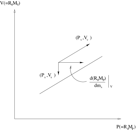
Figure 5: An illustration of the bare valence ($v$) and sea ($s$) quark mass dependence of pseudoscalar ($P$) and vector ($V$) meson masses in units of $R_{0}$.

As the valence quark mass parameter $m_{v}$ is varied, a curve is traced out. What is of interest, however, is the difference between such curves as the sea quark mass parameter $m_{s}$ is varied. Assuming, as discussed above, that the vector mass ($V\equiv R_{0}M_{V}$) is independent of $q_{s}$, then yields the required dependence of the pseudoscalar mass on $m_{s}$ at fixed $V$:

$$\left.{d(R_{0}M_{P})\over dm_{s}}\right|_{V}=P_{s}-{V_{s}\over V_{v}}P_{v}$$ (31)

We claim that this quantity will give the physically relevant part of the sea-quark dependence of meson masses: $d(R_{0}M_{P})/dq_{s}=r_{0}d(m_{P})/dq_{s})$. Indeed a presentation in this spirit was already shown in ref. [11]. There it was concluded that as the sea-quark mass is reduced, the meson masses move towards closer agreement with the experimental data point ($\eta_{s}$, $\phi$) with $d(R_{0}M_{P})/dm_{s}|_{V}>0$ (here $\eta_{s}$ is the mass expected for a $s\bar{s}$ pseudoscalar meson).

Since the precision we obtain in this preliminary study on the derivatives is not superior to that which was obtained by directly varying the sea and valence masses [11], the conclusions of that work are not modified. However, for dynamical fermion studies where only one sea-quark mass is employed, our methods will enable the derivatives with respect to the sea-quark mass to be evaluated.

6 Conclusions

One of the current problems in lattice study of hadron spectra, is to evaluate the physical consequences of including sea quark effects in the vacuum. We have presented lattice techniques to evaluate the dependence of meson masses on the valence and sea-quark parameters. These techniques allow such studies to be made using gauge configurations at a single set of lattice parameters. This is a significant advance for dynamical fermion studies which are very computationally intensive. Moreover it implies that some estimates of these sea-quark properties can even be made using quenched configurations.

We have discussed how to extract physically useful information about the sea-quark effects from these observables. Our proposal takes account of the changes induced in the lattice spacing and in the valence mass definition as the sea quark parameter is changed.

One rather encouraging feature is that we see evidence for a significant difference for the disconnected correlation ratio (our $D_{3}/C$) between quenched and dynamical quark configurations. It will be of interest to explore this difference at finer lattice spacing to establish that it is indeed a continuum effect.

7 Acknowledgements

We acknowledge the support from PPARC under grants GR/L22744 and GR/L55056 and from the HPCI grant GR/K41663.

Appendix A Appendix: Analysis of Z2 noise vector methods.

A.1 Introduction

We summarise first the salient ideas in the Z2 method [7, 8], before indicating the special features that we have made use of.

The required time-slice loop term can be expressed in terms of the quark propagator ${\cal M}^{-1}$ on a given gauge configuration as

$$T(t)=\sum_{x}{\cal M}^{-1}_{aj,aj}(x,t;x,t)$$ (32)

where we explicitly show the colour index $a$ and Dirac index $j$ here. Since ${\cal M}$ is $\gamma_{5}$-hermitian, then $T$ is real on any time-slice of any gauge configuration. To evaluate this expression for all $x$ on a time slice using point sources would require solving the lattice Dirac equation for $L^{3}$ sources of each colour and Dirac index. Let us instead explore using distributed sources $\xi^{p}(x,t)_{bk}$ where $p$ labels the source.

Then solving the lattice Dirac equation from such a source

$$G^{p}_{aj}(x^{\prime},t^{\prime})={\cal M}^{-1}_{aj,bk}(x^{\prime},t^{\prime};x,t)\ \xi^{p}_{bk}(x,t)$$ (33)

and combining with an appropriate combination involving the same source, we have

$${\cal T}^{p}(t)=\sum_{x}\xi^{p}_{aj}(x,t)^{*}\,G^{p}_{aj}(x,t)=\xi^{p}_{aj}(x,t)^{*}\,{\cal M}^{-1}_{aj,bk}(x,t;x^{\prime},t^{\prime})\ \xi^{p}_{bk}(x^{\prime},t^{\prime})$$ (34)

Interpreting the sources $\xi$ as random with specific properties then makes this quantity, averaged over realisations of the random source, to be just that required, namely

$$\langle{\cal T}^{p}(t)\rangle=T(t)$$ (35)

This allows the possibility of an unbiased estimate of the required quantity with a moderate number of inversions ($n_{Z}$). We require that the random sources $\xi^{p}_{aj}(x,t)$ with $p=1,\dots n_{Z}$ are such that the only non-zero expectation values of bilinears are given by

$$\langle\xi^{p}_{aj}(x_{1},t_{1})^{*}\ \xi^{q}_{bk}(x_{2},t_{2})\rangle=\delta_{pq}\delta_{ab}\delta_{jk}\delta_{x_{1},x_{2}}\delta_{t_{1},t_{2}}$$ (36)

This can be implemented by assigning an independent random number to each site $x$, colour $a$ and Dirac index $j$ for each sample $p$. The optimum distribution of those random numbers can be chosen to minimise the variance of the required observable.

The variance of this estimator is minimised [7] by taking Z2 noise (more correctly Z2$\times$Z2) , namely each component (for real and imaginary parts separately) to be randomly $\pm 1/\sqrt{2}$. Then

$$\sigma_{z}^{2}={1\over 2}{\rm Real}\left({\cal M}^{-1}_{ij}{\cal M}^{-1}_{ji}+{\cal M}^{-1}_{ij}{\cal M}^{-1*}_{ij}\right)_{i\neq j}$$ (37)

where only the off-diagonal part of ${\cal M}^{-1}$ contributes and here we include space, time, colour and Dirac indices into $i$.

The variance can be reduced by using a more selective source, for example [8] with specific Dirac components. This involves more inversions, however, if the full signal is to be evaluated. Here we choose, instead, to use a source which is only on a specific time-plane $t_{0}$. Thus in the above formalism $\xi^{p}(x,t)_{bk}$ is to be taken as zero outside the time-slice $t_{0}$ of interest. This reduces the variance by a factor of approximately 4 at the expense of 24 (in our case) times as many inversions. This is not cost-effective for evaluating $T$ but it does enable us to extract mesonic two-point correlators as we now discuss.

A.2 Meson correlators

It is also possible to use Z2 source methods to determine meson correlators. For illustration, consider the correlator between local hadron operators of zero momentum given by the average in the gauge configurations:

$$C(t)=\langle 0|H(t_{1})H^{{\dagger}}(t_{2})|0\rangle$$ (38)

with $t=|t_{1}-t_{2}|$ and where

$$H(t)=\sum_{x}\bar{\psi}_{aj}(x,t)\Gamma_{jk}\ \psi_{ak}(x,t)$$ (39)

creates a meson with quantum number given by the Dirac matrix $\Gamma$, where $\Gamma=\gamma_{5}$ for pseudoscalar mesons and $\Gamma=\gamma_{i}$ for vector mesons.

Then, using the $\gamma_{5}$-hermitian property of the fermion matrix, we need to evaluate (suppressing the colour indices)

$$C(t)=\sum_{x_{1},x_{2}}\langle 0|(\Gamma\gamma_{5})_{ij}{\cal M}^{-1}_{ik}(x_{1},t_{1};x_{2},t_{2})(\Gamma\gamma_{5})_{kl}{\cal M}^{-1*}_{jl}(x_{1},t_{1};x_{2},t_{2})|0\rangle$$ (40)

This can be evaluated using Z2 methods where $G^{p}(t)$ is the propagator from source $\xi^{p}$ on time-slice $t$ provided one also has the propagator $G^{p\Gamma}(t)$ from source $(\Gamma\gamma_{5})\xi^{p}$ on the same time-slice. Then the average over samples $p$ of this source will give the contribution to $C(t)$ from one time-slice on one gauge configuration:

$$C(t)=\langle\sum_{x_{2}}G_{i}^{p}(t_{1};x_{2},t_{2})G_{j}^{p\Gamma*}(t_{1};x_{2},t_{2})(\Gamma\gamma_{5})_{ij}\rangle$$ (41)

This method allows us to obtain mesonic correlators from any time slice to any other. For the pseudoscalar meson, no additional inversions are needed since $\Gamma\gamma_{5}=1$ in that case. For the vector meson case, we use $\Gamma=\gamma_{i}$ with $i=1,2$ or 3 randomly chosen for each sample $p$.

In principle, one could obtain mesonic correlations using Z2 methods without additional inversions - for example by explicitly evaluating the average over samples $p,\ q$ of

$$\sum_{x_{2}}G^{p}_{i}(t_{1};x_{2},t_{2})\Gamma_{ij}\xi^{q*}_{j}(x_{2},t_{2})\times\sum_{x_{1}}G^{q}_{k}(t_{2};x_{1},t_{1})\Gamma_{kl}\xi^{p*}_{l}(x_{1},t_{1})$$ (42)

In this case, combinatorial factors make the variance of this estimator comparable to the signal so it is an inefficient estimator. Using sources at all $t$ would aggravate this problem considerably.

As described in the text, we can combine the Z2 estimate of the loop at $t_{0}$ with the Z2 estimate of the mesonic correlator, provided $t_{0}$ is not the source point of the mesonic correlator determination. This restriction is of no consequence since we are interested in a loop roughly midway along the mesonic correlator.

A.3 Propagators from Z2 sources

.

The techniques used to evaluate the propagator from a given Z2 source are just those used in a standard inversion from any source. This is achieved by an iterative inversion process (either minimal residual or BiCGstab algorithms were used). The special feature is that the precision needed in this iteration is such that any biases are at a level substantially below the statistical noise from the Z2 method. We are able to monitor several quantities of interest (eg. ${\rm Trace}{\cal M}^{-1}$ on a time slice and the pion propagator to large $t$) continuously during the iterative inversion process. The convergence of these quantities of interest during the iterative process is not monotonic, but we are able to establish a value of the residual that guarantees sufficiently small systematic errors from lack of convergence. In practice we need approximately one half of the number of iterations used in a conventional inversion. This has also been discussed by the SESAM collaboration [8].

References

- [1] UKQCD Collaboration, P. Lacock et al., Phys. Rev. D 52, 5123 (1995).
- [2] UKQCD Collaboration, A.C. Irving et al., hep-lat/9807015.
- [3] C. Michael, Nucl. Phys. B280 [FS18], 13 (1987).
- [4] G. Bali, C. Schlichter and K. Schilling, Phys. Lett. B363, 196 (1995).
- [5] UKQCD Collaboration, C. Michael, J. Peisa, hep-lat/9802015.
- [6] G.M. de Divitiis, R. Frezzotti, M. Masetti, R. Petronzio, Phys. Lett. B 382, 393 (1996).
- [7] S. Dong et al., Phys. Rev. D54, 5496 (1996); K.F. Liu et al., PRL74 (1994) 2172; Phys. Rev. D49, 4755 (1994); S.J. Dong and K.F. Liu., Phys. Lett. B328, 130 (1994).
- [8] SESAM Collaboration, N. Eicker et al., Phys. Lett. B389 (1996) 720; J. Viehoff et al., Nucl. Phys. B (Proc. Suppl.) 63, 269 (1998).
- [9] UKQCD Collaboration, H. Shanahan et al., Phys. Rev. D 55, 1548 (1997).
- [10] UKQCD Collaboration, P. Lacock, A. McKerrell, C. Michael, I.M. Stopher, P.W. Stephenson, Phys. Rev. D 51, 6403 (1995).
- [11] UKQCD Collaboration, C. Allton et al., hep-lat/9808016.
- [12] Alpha Collaboration, M. Guagnelli et al., hep-lat/9806005.