Magnetic Monopole Content of Hot Instantons

Abstract

We study the Abelian projection of an instanton in $R^{3}\times S^{1}$ as a function of temperature (T) and non-trivial holonomic twist ($\omega$) of the Polyakov loop at infinity. These parameters interpolate between the circular monopole loop solution at $T=0$ and the static ’t Hooft-Polyakov monopole/anti-monopole pair at high temperature.

1 INTRODUCTION

Although many qualitative features of QCD are well described by a vacuum state dominated by an instanton “liquid’, confinement appears to be an exception [1]. Instead, magnetic monopoles are thought to be the crucial ingredient. This raises the question of how magnetic degrees of freedom can be incorporated into (or reconciled with) an instanton “liquid”. A recent step in this direction was taken by Brower, Orginos and Tan (BOT)[2] who studied in detail the magnetic content of a single isolated instanton, defining magnetic currents via the Maximally Abelian (MA) projection. They found a marginally stable direction for the formation of a monopole loop. Now with the more general caloron solution of T. Kraan and P. van Baal [3], and K. Lee and C. Lu [4], this analysis can be extended to an isolated SU(2) instanton at finite temperature ($T$) with a non-trivial holonomy ($\omega$) for the Polyakov loop.

Figure 1: Magnetic monopole phase plane for the caloron in polar co-ordinates: $(\rho T,2\pi\omega)$.

The resultant picture that emerges is appealing (see Fig. 1). For $\omega=0$, the small monopole loop at the core of a cold instanton grows in size as one increases the temperature and is transformed into a single static ’t Hooft-Polyakov monopole at infinite temperature, as noted earlier by Rossi [5]. Note that the other quadrants of Fig. 1 can be found by applying $Z_{2}$ center symmetry ($\omega\rightarrow\omega+{\textstyle{1\over 2}}$) and monopole to anti-monopole charge conjugation ($\omega-{\textstyle{1\over 4}}\rightarrow{\textstyle{1\over 4}}-\omega$).

The MA projection provides a fully gauge and Lorentz invariant definition of monopole currents by introducing an auxiliary adjoint Higgs field, $\vec{\phi}(x)$, fixed at the classical minimum,

$$G={\textstyle{1\over 2}}\int[(D_{\mu}(A)\vec{\phi})^{2}+\lambda(\vec{\phi}\cdot\vec{\phi}-1)^{2}]d^{4}x\;,$$ (1)

in a fixed background gauge field, $A_{\mu}$. This yields the Abelian projected field strength,

$$f_{\mu\nu}={\mathbf{n}}\cdot{\mathbf{F}}_{\mu\nu}-{\mathbf{n}}\cdot D_{\mu}{\mathbf{n}}\times D_{\nu}{\mathbf{n}}\;,$$ (2)

with its U(1) monopole current,

$$k_{\mu}=\frac{1}{4\pi}\partial_{\nu}\tilde{f}_{\nu\mu}\rightarrow\frac{1}{8\pi}\epsilon_{\mu\nu\rho\sigma}\partial_{\nu}{\mathbf{n}}\cdot\partial_{\rho}{\mathbf{n}}\times\partial_{\sigma}{\mathbf{n}}\;,$$ (3)

where ${\mathbf{n}}(x)\equiv\vec{\phi}(x)/|\phi(x)|$. It is conventional to identify the MA gauge by the rotation $\Omega(x)$ in the coset $SU(2)/U(1)$ that aligns ${\mathbf{n}}$ along the 3 axis. We have extended the conventional Abelian projection ($\lambda=\infty$) to a continuous family including the analytically more tractable BPS limit ($\lambda=0$), where the difficult problem of minimizing the MA functional $G$ reduces to an eigenvector problem for the Higgs field, $D_{\mu}(A)^{2}\vec{\phi}_{E}=E\vec{\phi}_{E}$.

2 COLD MONOPOLE LOOP

We begin at the origin of Fig. 1, where there is a single isolated instanton at zero temperature. A trivial, but essential, observation is that the singular gauge instanton in the ’t Hooft ansatz,

$$A^{a}_{\mu}=\bar{\eta}^{a}_{\mu\nu}\partial_{\nu}\log(1+\rho^{2}/x^{2}).$$ (4)

is also the MA projection which minimizes the Higgs action $G$. In the BPS limit, this is equivalent to having a zero eigenvalue solution,

$$\vec{\phi}_{0}(x)=\frac{x^{2}}{x^{2}+\rho^{2}}[0,0,1],$$

for the Higgs field aligned with the 3-axis. Consequently there is no magnetic content to the MA projection. This would be the entire story except that there is another zero eigenvalue that implies a flat direction for the formation of an infinitesimal monopole loop.

The geometry of this loop is interesting. The gauge singularity at the origin is caused by a rotation, $g(x)=x_{\mu}\tau_{\mu}/|x|$ and $\tau_{\mu}=(1,i\vec{\tau})$. Locally it is advantageous to “unwind” this singularity to a distance R further reducing the MA functional $G$. This almost wins, creating a monopole loop of radius R which only slightly increases G, $\delta G/G\simeq R^{4}\log(R)$. Almost any local disturbance, due to a nearby instanton for example, will stabilize the loop [2]. The second zero mode vector in the BPS limit is easily constructed using conformal invariance.

$$\vec{\phi}_{1}(x)=\frac{1}{x^{2}(x^{2}+\rho^{2})}[\sin\beta\cos\alpha,\sin\beta\sin\alpha,\cos\beta],$$

where $\alpha=\varphi-\psi$ , $\cos\beta=(v^{2}-u^{2})/(u^{2}+v^{2})\;$, with $x_{1}+ix_{2}=ue^{\textstyle{i\varphi}}$, $x_{3}+ix_{0}=ve^{\textstyle{\psi}}$.

The superposition of the two zero modes produces a loop. Finally note that the topological charge is related to the magnetic charge, through a surface term on the boundary of the loop, $\Sigma$,

$$Q\rightarrow\int_{\Sigma}\frac{Tr[\Omega_{R}d\Omega_{R}^{\dagger}\wedge\Omega_{R}d\Omega_{R}^{\dagger}\wedge\Omega_{R}d\Omega_{R}^{\dagger}]}{24\pi^{2}}\;,$$

where $\Omega_{R}$ is the singular gauge transformation providing a Hopf fibration for the infinitesimal “non-contractible” loop.

3 HOT BPS MONOPOLES

At low temperature with $\omega=0$ the MA projection is similar. The periodic instanton in the ’t Hooft ansatz,

$$A^{a}_{\mu}\!\!=\!\bar{\eta}^{a}_{\mu\nu}\partial_{\nu}\log\!\left(\!1\!+\frac{\pi T\rho^{2}\sinh(2\pi Tr)}{2r(\sinh^{2}(\pi Tr)+\sin^{2}(\pi Tt))}\!\right)\!,$$

is again equivalent to the MA projection. “Unwinding” the periodic copies of the singularities at $x=0$ is now accomplished by $g=X_{\mu}\tau_{\mu}/|X|\;,\;X_{\mu}=[\tan(\pi Tt),\hat{r}\tanh(\pi Tr)]$, leaving a monopole loop. However surprisingly at infinite temperature, or equivalently $\rho=\infty$ as noted by Rossi, the instanton is gauge equivalent to the static ’t Hooft-Polyakov monopole solution. With ${\mathbf{n}}(x)=\hat{r}$, this is the correct MA projection (or unitary gauge). For the case of the BPS limit, the solution is simply $\vec{\phi}(x)\equiv\vec{A}_{0}(x)$, as one might expect. Consequently the MA projection correctly identifies the standard static monopole.

4 CALORON $\bf T$-$\bf\omega$ PLANE

For $\omega\neq 0$, we encounter the full complexity of the new caloron solution [3],

$$A_{\mu}\!\!=\!\tau^{3}\bar{\eta}^{3}_{\mu\nu}\partial_{\nu}\log\phi(x)\!+\!(\tau^{+}\bar{\eta}^{-}_{\mu\nu}\partial_{\nu}\chi(x)\!+\!c.c.)\psi(x),$$

in the singular gauge. In the limit of $T\rightarrow\infty$, we have verified that MA projection now gives a pair of ’t Hooft-Polyakov BPS monopole/anti-monopole separated by distance $D=\pi\rho^{2}T$ as expected. However, now the singular gauge caloron no longer satisfies the MA projection and it is difficult to find the MA projection analytically. Thus we have minimized G numerical in the interior of the $T-\omega$ phase plane of Fig. 1 by placing the functional on a grid.

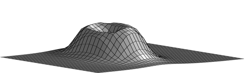
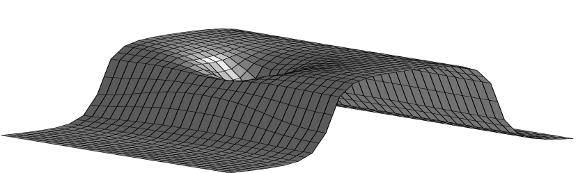
Figure 2: Profiles of $\beta(0,z,t)$ at $\omega=.125$ for a loop (top, $\rho T=0.56$) and for monopole/anti-monopole pair (bottom, $\rho T=0.57$).

On symmetry grounds, one can prove the existence of cylindrical solutions with $\alpha=\varphi+\tilde{\alpha}(u,z,t)\;,\;\beta(u,z,t)$. The Dirac sheet is located by a jump in $\beta(t,x)$ by $\pi$. In Fig. 2, we give the profile for $\beta(u,z,t)$ in the z-t plane slicing through the instanton centered at $u=0$.

Figure 3: The area $A$ of the minimal spanning Dirac sheet versus temperature $T$ for $\omega=0.125$.

To explore further the transition from the monopole loop to a pair of monopole lines, we plot in Fig. 3 the area of the minimal spanning Dirac sheet. At $\rho T\simeq 0.56$, there is a clear transition separating the two regimes.

Based on the absence of a loop for a single isolated instanton [2], we anticipate that the formula for the size of the loop (or separation of the lines) must involve a new length scale, $L$. This scale represents the distance to nearby perturbations such as the anti-instanton presented in Ref. [2]. For the single caloron plotted here, the new scale is $L=\beta=1/T$ . This suggests a simple scaling form: $R\sim\rho(\rho T)^{\gamma}$ with $\gamma>0$. Indeed in Fig. 3 for $(\rho T)^{2}<0.32$, we do see a positive curvature for the area, $A/\beta^{2}\sim(RT)^{2}\sim(\rho T)^{2+2\gamma}$, i.e., $\gamma>0$, consistent with our expectation. On the other hand, at high temperatures, the monopole/anti-monopole trajectories are known [3, 4] to be separated asymptotically by $D=\pi\rho(\rho T)^{\gamma}$ with $\gamma=1$, which is also confirmed by a linear fit to $A=D\beta\simeq\pi\rho^{2}$ for $(\rho T)^{2}>0.3$.

Finally it is interesting to note that the kinematical “transition” seen in Fig. 3 is near to the Yang-Mills deconfinement temperature for a typical instanton size of ${\textstyle{{1}\over{3}}}$ fermi. However, a serious analysis of deconfinement dynamics and its possible relations to the monopole content of the caloron is left to future investigations.

References

- [1] Talks by J. W. Negele and D. Chen at this conference.
- [2] R. Brower, K. Orginos and C-I Tan, Phys. Rev. D55 (1997) 6313.
- [3] T. Kraan and P. van Baal, “Periodic Instantons with non-trivial Holonomy”, hep-th/9805168.
- [4] K. Lee and C. Lu, Phys.Rev. D58 (1998) 025011.
- [5] P. Rossi, Nucl. Phys. B149 (1979) 170.