Abstract

Qualitative features of Ginsparg-Wilson fermions, as formulated by Neuberger, coupled to two dimensional $U(1)$ gauge theory are studied. The role of the Wilson mass parameter in changing the number of massless flavors in the theory and its connection with the index of the Dirac operator is studied. Although the index of the Dirac operator is not related to the geometric definition of the topological charge for strong couplings, the two start to agree as soon as one goes to moderately weak couplings. This produces the desired singularity in the quenched chiral condensate which appears to be very difficult to reproduce with staggered fermions. The fermion determinant removes the singularity and reproduces the known chiral condensate and the meson mass within understandable errors.

1. Introduction

Our understanding of chiral symmetry on the lattice has matured recently. The overlap formulation [1] has lead to a new Dirac operator that is expected to describe exactly massless fermions [2]. The chiral symmetry on the lattice that makes this possible has been discovered in Ref. [3]. This symmetry arises when the Dirac operator $D$ satisfies

$$D\gamma_{5}+\gamma_{5}D=D\gamma_{5}D,$$ (1)

called the Ginsparg-Wilson relation [4]. This relation appears to be quite powerful. It helps to reproduce the continuum relations arising due to chiral symmetry, and thus leads to elegant renormalization properties [5]. Further, like in the continuum, it also suggests an elegant resolution of the $U(1)$ problem on the lattice which has interesting consequences for the lattice calculations of QCD [6]. We will refer to the fermion formulations which obey the Ginsparg-Wilson relation as Ginsparg-Wilson fermions.

In addition to the Neuberger operator [7], the fixed point Dirac operator also obeys the Ginsparg-Wilson relation [8]. Here we do not discuss the latter approach. In the context of the Neuberger’s Dirac operator it is important to point out that there is another closely related approach to massless fermion based on an extension [9] of an idea of Kaplan [10] called domain wall fermions. These fermions can be considered as a truncated version of the overlap [11]. The appropriate Dirac operator of domain wall fermions satisfy the Ginsparg-Wilson relation up to exponentially small violations in the limit where the separation of the walls, on which the physical fermions live, becomes large. The domain wall fermions have been used in QCD calculations [12] and appear to have very good chiral properties compared to the Wilson fermion approach. More recently this approach has also been shown to reproduce some of the singularities in the chiral condensate due to exact zero modes that have not been seen in staggered fermion formulations [13]. Thus the domain wall fermions appear to be a practical way to implement the Ginsparg-Wilson relation approximately. However, in this article we explore the possibility of keeping the Ginsparg-Wilson relation exact by working directly with Neuberger’s Dirac operator.

Although chiral symmetry emerges naturally with Ginsparg-Wilson fermions, their dynamical consequences are just beginning to be explored. The first study of the fixed point Dirac operator was done in the Schwinger model in Ref. [14]. A similar study for Neuberger’s Dirac operator is lacking. Tests performed in closely related formulations like the overlap [16] and domain wall fermions [17] can only be used to gain confidence, since all these formulations differ in their cutoff effects. In Neuberger’s Dirac operator such effects enter through a mass parameter $M$. It is important to understand such effects and check for universality. This has not yet been done. Further, in the context of the Schwinger model, the studies in the overlap and domain wall formulations have only concentrated on the chiral condensate [18, 19]. The meson mass has been ignored. As we discuss below, this is another important quantity to calculate to confirm universality.

A new feature of the Ginsparg-Wilson fermions is that the Dirac operator has a non-zero coupling between any two lattice points which are exponentially small in the distance between the points [20]. Such actions are still considered local if they do not destroy the mass spectrum of the theory. This can be checked in the free theory. On the other hand it is important to see if this feature continues at a non-perturbative level and no spurious long range correlations originate. This question has been recently addressed for smooth gauge fields in Ref. [21]. Non-perturbatively one can study the mass spectrum of the theory. Thus determining the meson mass in the Schwinger model is important to confirm our beliefs.

In this article we study a two dimensional $U(1)$ lattice gauge theory coupled to fermions proposed by Neuberger [2]. In the continuum limit, this model approaches the Schwinger model up to four-Fermi couplings [19]. To control these couplings is quite difficult. and will not be attempted here. Instead we will try to learn qualitative features of the model as a way to learn how it could reproduce the main properties of the Schwinger model if a more thorough and complete analysis is made. We also leave the more interesting multi- flavor case to later studies since there the dynamics is considerably more complicated and finite volume effects must be carefully studied before the effects of complete chiral symmetry guaranteed by Neuberger’s Dirac operator can be understood. In particular it is important to obtain results like $\langle\bar{\psi}\psi\rangle\sim m^{1/3}$ and the pion mass $\sim m^{2/3}$ [22, 17].

This article is organized as follows. In section 2 we introduce the model. In section 3 we discuss the role of the Wilson mass parameter that enters the definition of the Dirac operator. In particular we show an interesting relation between the zero modes of the Dirac operator and the number of fermion flavors that the theory describes for background gauge field configurations. In section 4 we discuss the connection between topology and index of the Dirac operator. This was recently studied for semi-classical gauge field configurations in Ref. [24]. Here we understand this connection as a function of the gauge coupling. We then argue that this is responsible for reproducing the singularities of the quenched approximation. In section 5 we calculate the spectral density of the Dirac operator as a function of the fermion mass. We also calculate the chiral condensate and the meson mass after including the fermion determinant and compare it with the results in the Schwinger model. A short discussion showing the relevance of the results to QCD and directions for future work are pointed out in section 6.

2. The Model

The model that we investigate can be described by the action

$$S=\beta\sum_{\cal P}\left(1-\frac{1}{2}[U_{\cal P}+U_{\cal P}^{\dagger}]\right)+\sum_{x,y}\bar{\Psi}_{x}[D_{x,y}+m\delta_{x,y}]\Psi_{y}$$ (2)

where $U_{\cal P}$ is the phase obtained by multiplying the four $U(1)$ phase angles attached to a plaquette and $\beta=1/g^{2}$ is the gauge coupling. Fermions of mass $m$ interact with the gauge fields through the Dirac operator $D$, chosen to be the one proposed by Neuberger [2]. In terms of the hermitian Wilson-Dirac operator

$$H_{x,y} = -\frac{\gamma_{5}}{2}\left(\delta_{x,y-\hat{\mu}}U^{\dagger}_{\mu}(x)\left[1-\gamma_{\mu}\right]+\delta_{x,y+\hat{\mu}}U_{\mu}(y)\left[1+\gamma_{\mu}\right]\right)+\delta_{x,y}\gamma_{5}(2+M),$$ (3)

with the mass parameter $M$, $D$ is given by

$$D=1+\gamma_{5}H/\sqrt{H^{\dagger}H}.$$ (4)

It is easy to show that $D$ satisfies eq.(1). The fermions obey (anti)periodic boundary conditions in the (temporal) spatial directions and the gauge fields are periodic.

The condensate that characterizes chiral symmetry breaking was defined in Ref. [6]. After integrating out the fermions this can be written as

$$\langle\bar{\psi}\psi\rangle=Z\frac{1}{L_{s}L_{t}}\left\langle{\rm Tr}\left[(1-\frac{D}{2})\frac{1}{D+m}[{\rm Det}(D+m)]^{N_{f}}\right]\right\rangle/\langle[{\rm Det}(D+m)]^{N_{f}}\rangle$$ (5)

where $L_{s},L_{t}$ are the lattice sizes in the spatial and temporal directions and $Z$ takes care of the wave function normalization. $N_{f}$ is the number of flavors. $N_{f}=0$ corresponds to the quenched theory. We do not consider $N_{f}\geq 2$ in this article.

All our calculations are performed on an $8\times 16$ lattice. Gauge fields are generated by a combination of head bath and over relaxation algorithm. Every gauge field configuration is generated after 500 sweeps (one sweep = one heat bath update + 5 over-relaxation step over the entire lattice). The fermion determinants are absorbed into the observable and the expectation value is taken over gauge field configurations generated with the Boltzmann weight of the pure gauge theory. Although not a very reliable method for large lattices, the procedure seems to produce results with controlled errors in the present calculation. This is because the physics of the one flavor model is mainly sensitive to topology and the fermion determinant within a topological sector does not fluctuate much. Further these sectors are updated well with the above algorithm on lattice sizes such as ours. Calculations involve a statistics over 2500 independent gauge field configurations. The errors are obtained through a jack-knife procedure.

The model contains three additional parameters. The coupling $g=1/\sqrt{\beta}$ controls the lattice spacing. Since $g$ is dimensionful in two dimensions, $g\sim 1/a$. The continuum limit of this model is reached in the $\beta\rightarrow\infty$ limit. The mass parameter $M$ does not effect the fermion mass, which is determined by $m$. It controls the effects of the fermion doubling. We will clarify its role further in the next section. Since it is difficult to control the four Fermi-couplings induced by the above model, it is considerably more difficult to do a systematic continuum extrapolation. Based on results in Ref. [19] it is likely that in the continuum limit the above model will show differences with the results in the Schwinger model at the $10\%$ level. Hence we study the model at a fixed $\beta$, which also introduces finite lattice spacing errors. As we will see the results from the present study differ from the Schwinger model by $10\%-15\%$, and based on the above discussion can be considered understandable.

3. The role of $M$

The parameter $M$ is the mass of the Wilson Dirac operator that enters the definition of $D$. The theory can describe massless fermions for a range of values of $M$. Interestingly, as $M$ changes it can change the number of massless fermions in the theory and thus can reintroduce fermion doubling. This happens at some critical values, say $M_{c}$. It is easy to understand this in the free theory by analyzing the propagator. The free propagator at $M=-1$ was constructed in Ref. [24]. Extending this result to arbitrary $M$ we get

$$S_{F}(p)=\frac{1}{2}-\frac{i\gamma_{\mu}\sin(p_{\mu})}{2[N(p)+u(p)]}$$ (6)

where $-\pi<p\leq\pi$, with

$$u(p)=2+M-\sum_{\mu}\cos(p_{\mu}),\;\;\;N(p)=\sqrt{u^{2}(p)+\sum_{\mu}\sin^{2}(p_{\mu})}$$ (7)

When $M>0$ there are no massless particles. For $-2<M<0$ the only pole in the propagator describing massless particles is at the origin of the $(p_{1},p_{2})$ plane. However, in the region $-4<M<-2$ two additional poles appear at $(\pi,0)$ and $(0,\pi)$. Here the Dirac operator describes three flavors of massless fermions. Finally for $M<-4$ a fourth pole at $(\pi,\pi)$ also appears and the theory describes four massless fermions. Thus the theory can describe different phases which are distinguished by the number of massless fermion flavors. In the free theory the critical values $M_{c}=0,-2$ and $-4$ separate these phases. The number of massless flavors in the various phases discussed here differ from the those in domain wall fermions when the extra dimension is discrete [25]. This question was recently investigated by Shamir who observes the above results in the limit where the lattice spacing in the extra dimension becomes zero [26].

The critical values of $M_{c}$ will fluctuate in the presence of gauge fields. It is important to find a region in $M$ in the full interacting theory where one can isolate the one flavor phase. In the weak coupling limit such a phase is most likely to exist. Since this also coincides with the continuum limit, both for the present model and in QCD, it is likely that one can actually obtain the physics of one flavor, sufficiently close to the continuum. On the other hand in realistic calculations it will be important to establish this before the results can be trusted. We will show that there is an interesting connection between the index (or equivalently the number of zero modes with a given chirality) and the number of massless fermions described by the Dirac operator in a background gauge field configuration at a given value of $M$. It may be possible to use this connection to determine the values of $M$ that belong to the one flavor phase for each given background gauge field configuration.

Consider a background gauge field configuration with a non-trivial index in the one flavor phase. As we cross a critical value of $M$ the index can change. Such effects have been studied recently in Ref. [27]. The change appears to be related to the change in the number of massless flavors the Dirac operator describes. We can predict it as a function of $M$ based on this relationship. For example, let $\nu\neq 0$ be the index of $D$ in the one flavor phase. In the three flavor phase, we expect massless fermions from the poles at $(0,0)$, $(\pi,0)$ and $(0,\pi)$. However, the chirality definition of the fermions with poles at $(\pi,0)$ and $(0,\pi)$ are opposite to that of $(0,0)$ and $(\pi,\pi)$. This means that in the three flavor phase the index of $D$ will be $-\nu$. A similar argument shows that the index of the operator in the four flavor case would be zero. Since the operator is designed to produce zero modes equal to the index, this means that the Dirac operator will not have any (except accidental) zero modes in the zero and four flavor phases and will have $\nu$ zero modes of opposite chirality in the one and three flavor phases. Thus one can scan through $M$ to find the four phases for any gauge field with a non-zero index. In order to check the above observations numerically, we generated a series of gauge field configurations at $\beta=3.$ on a $8\times 16$ lattice. In table 1 we give values of the index of the Dirac operator for ten such configurations for four values of $M$ in the various phases. The results indicate that $M=-1.0$ is a region dominated by the physics of one fermion flavor, when $\beta\geq 3.$

	Index
Gauge Action	M=1.0	M=-1.0	M = -3.0	M = -5.0
0.1665	0	-1	1	0
0.1589	0	1	-1	0
0.1962	0	3	-3	0
0.1669	0	0	0	0
0.1822	0	0	0	0
0.2309	0	-1	1	0
0.1933	0	2	-2	0
0.1904	0	0	0	0
0.1753	0	1	-1	0
0.1527	0	0	0	0

Table 1: The table shows the index of the Dirac operator as a function of the Wilson mass $M$. The connection of the index with the number of massless fermion flavors and their chiralities is responsible for the above results. The first column indicates the value of the plaquette term of eq.(2) for the various configurations used. The results are consistent with theoretical predictions.

As far as we know, the above connection between the index of the Dirac operator and the number of fermion flavors has not been appreciated before. In fact this connection leads to an amusing conjecture. In the region $M<-4$ there are four massless flavors but the Dirac operator does not produce any zero modes related to topology. The zero modes, if they exist, are accidental. However, there is a $U(1)$ chiral symmetry in the action because the operator obeys the Ginsparg-Wilson relation [3]. Since there are no zero modes to break the symmetry through the measure, the exact chiral symmetry present must be flavored and hence not anomalous. This reminds one of staggered fermions where such a symmetry exists although the theory describes two flavors of massless fermions .

In addition to producing the different phases, $M$ is expected to renormalize the relevant couplings including the gauge coupling and the fermion mass. In fact it also introduces a wave-function renormalization. This can be seen by expanding the fermion propagator in small momenta near the poles in the various phases. We get

$$2[N(p)+u(p)]=\left\{\begin{array}[]{cc}\frac{1}{|M|}(p_{1}^{2}+p_{2}^{2})+...&\hbox{expansion near}\;(0,0),\;\;M<0\\ \frac{1}{|2+M|}(p_{1}^{2}+p_{2}^{2})+...&\hbox{expansion near}\;(0,\pi)\;\;{\rm or}\;\;(\pi,0),\;\;M<-2\\ \frac{1}{|4+M|}(p_{1}^{2}+p_{2}^{2})+...&\hbox{expansion near}\;(\pi,\pi),\;\;\;M<-4\\ \end{array}\right.$$ (8)

This shows that the wave-function renormalization at tree level turns out to be $Z=1/|M|$ in the one flavor phase. As we will see below, the dominant effect of $M$ on the chiral condensate of eq.(5) comes from $Z$. Interestingly, we see that the residue at the various poles are different showing that the various massless fermions can have different wavefuntion renormalization constants. This suggests that the renormalization properties of the three and four flavor phases needs to be understood further before they can be treated as a regularized version of legitimate field theories.

4. Zero Modes and Quenching

The one flavor Schwinger model is mainly governed by the dynamics of the gauge field topology and its connection with zero modes of the Dirac operator through the index theorem. Previous studies have shown that Ginsparg-Wilson fermions can reproduce the index theorem easily. We confirm this here. We choose the geometric definition of the topological charge given by

$$Q=\frac{1}{2\pi}\sum_{\cal P}\log(U_{\cal P})$$ (9)

where the value of the log is defined on the principal sheet, i.e., $0\leq\log(U_{\cal P})<2\pi$. For smooth fields one expects that the index of the Dirac operator will be related to the above definition of the topological charge [24]. For rough fields there is no reason for such a relation. In order to quantify this effect we compared Q with the index of the Dirac operator at a strong coupling $\beta=0.5$ and a moderately weak coupling $\beta=3.0$ lattice. The results for fifty configurations are plotted in the figure (1). These results show that even though the index of the Dirac operator is not related to the geometrical definition in any formal sense, the two start to agree quite well at moderately weak couplings and that $\beta=3$ is sufficiently weak to reproduce the topological properties of the two dimensional theory. In figure (2) we plot the histogram for the topological sectors obtained from an ensemble of 2500 configurations at $\beta=3$. This further shows that the algorithm samples the various topological sectors adequately.

The realization of the index theorem on the lattice has important consequences. In QCD it is well known that the mass of the $\eta^{\prime}$ particle is a consequence of the dynamics of the zero modes of the Dirac operator. In the quenched theory the zero modes are enhanced since the suppression of these modes due to the fermion determinant is absent. This causes many interesting singularities in the theory. In the infinite volume limit, these singularities have been predicted based on quenched chiral perturbation theory in Ref. [28]. At small volumes semi-classical expansions suggest that there will be instanton like configurations that will dominate the path integral and this will lead to exact zero modes of the Dirac operator. This leads to new singularities. One of the consequences is the divergence of the quenched chiral condensate.

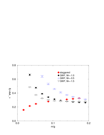
Figure 3: The chiral condensate including the factor $Z=1/|M|$ in the quenched limit is shown. For comparison we also include the results from staggered fermion simulations.

The divergence of the quenched chiral condensate in the Schwinger model has been discussed in Ref. [29]. The condensate was first calculated in Ref. [30] using staggered fermions on a $16\times 16$ lattice. The divergence as a function of the fermion mass was not found and was completely ignored even in the discussion. The singularity was first discussed in some detail in Ref. [31] where simulations on $64\times 64$ lattices were reported. These calculations have not been confirmed by other groups. Recent studies in QCD suggest that such singularities are difficult to obtain with staggered fermions [32, 33], but appear rather easily in the domain wall formalism [13]. The above discussion of the index theorem shows that with Ginsparg-Wilson fermions these divergences must appear easily. In order to show the dramatic difference between staggered fermions and the Ginsparg-Wilson fermions, we plot the quenched chiral condensate as a function of the fermion mass in figure (3) for both types fermions.

5. Dirac Spectral Density and Meson Mass

The study of the chiral condensate and the meson mass is important in any study of the Schwinger model. The chiral condensate is given by eq.(5). Written in terms of the eigenvalue density $\rho(\theta)$ of the Dirac operator [6], it reads

$$\langle\bar{\psi}\psi\rangle=Z\int_{-\pi}^{\pi}d\theta\;\rho(\theta)\frac{1+\cos(\theta)+i\sin(\theta)}{2(1-\cos(\theta)-i\sin(\theta)+am)}.$$ (10)

In deriving the above representation, we have used the fact that the eigenvalues of the Ginsparg-Wilson Dirac operator are distributed on a unit circle in the complex plane centered at $(1,0)$. The density is normalized using the relation $\int d\theta\rho(\theta)=2$.

An eigenvalue at $\theta=0$ is an exact zero mode. It is easy to see that every eigenvalue at $\theta=0$ will be accompanied by an eigenvalue at $\theta=\pi$ for topological reasons. Separating these topological zero modes, we find

$$\rho(\theta)=\rho_{0}\left[\delta(\theta)+\delta(\theta-\pi)\right]+\rho^{\prime}(\theta)$$ (11)

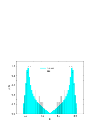
Figure 4: This figure shows the eigenvalue density of $D$ for the quenched run at $\beta=3.0$ and for free field theory.

In figure (4) we plot $\rho^{\prime}(\theta)$ at $\beta=3.0$ and $|M|=1.0$ obtained using quenched configurations. For comparison we also plot the free field eigenvalue density.

It is useful to understand the dependence of $\rho(\theta)$ on the dynamical fermion mass. Since all the eigenvalues are measured, this is easily obtained. For each configuration we divide the range $(-\pi,\pi)$ into 50 bins and count the number of eigenvalues falling into each bin and divide it by $(L_{s}L_{t})2\pi/50$ to obtain the value of $\rho^{\prime}(\theta)$ where $\theta$ refers to the center of the bin. For $\theta=0$ we give the value of $\rho_{0}$ which is obtained by counting the zero modes and dividing by the $L_{s}L_{t}$. $\rho(\theta)$ for four values of the dynamical fermion mass is given in table 2. The errors are obtained by a jackknife method. $\rho(\theta)$ is even and we give the values for positive $\theta$. From the results it appears that the statistics of 2500 configurations is far from sufficient to see the effects of the fermion determinant except in the region $|\theta|<0.35$. This corresponds to masses less than 0.06 in lattice units.

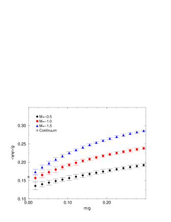
Figure 5: The chiral condensate including the factor $Z=1/|M|$ is plotted as a function of the fermion mass for various values of $M$. The dominant role of $|M|$ comes through $Z$. The continuum value in the massless Schwinger model is shown on the $m/g=0$ axis.

The chiral condensate is evaluated for three different values of $M$, in the one flavor phase, in order to study its effects. The dominant effect comes from the tree level wave function renormalization factor $Z=1/|M|$. This factor will get corrections from loop effects. The results after including this factor are shown as a function of the fermion mass in figure (5). In the continuum it can be shown that

$$\frac{\langle\bar{\psi}\psi\rangle}{g}=\frac{{\hbox{\rm\bf C}}}{2\pi\sqrt{\pi}},$$ (12)

where ${\hbox{\rm\bf C}}=1.78107...$ is the Euler’s constant. This is indicated on the $m=0$ axis. As discussed in section 2, it will be difficult to reproduce the results of the Schwinger model with errors of less than $10-15\%$ from the present lattice study. Our results are consistent with this expectation.

$\theta$	$\rho(\theta)$
	m=0.01	m = 0.1	m = 1.0	quenched
3.0788	0.180(08)	0.189(04)	0.209(01)	0.2110(12)
2.9531	0.411(22)	0.395(09)	0.384(02)	0.3839(10)
2.8274	0.655(38)	0.648(17)	0.638(03)	0.6379(11)
2.7018	0.926(60)	0.922(33)	0.914(03)	0.9130(09)
2.5761	0.978(52)	0.970(23)	0.960(03)	0.9590(11)
2.4504	0.755(44)	0.762(18)	0.770(02)	0.7697(09)
2.3248	0.573(34)	0.583(22)	0.596(03)	0.5965(16)
2.1991	0.503(28)	0.498(12)	0.495(02)	0.4948(10)
2.0735	0.431(25)	0.425(11)	0.417(02)	0.4176(11)
1.9478	0.370(22)	0.364(09)	0.359(02)	0.3590(12)
1.8221	0.310(17)	0.310(07)	0.312(02)	0.3130(13)
1.6965	0.264(15)	0.270(07)	0.277(02)	0.2774(14)
1.5708	0.236(15)	0.240(06)	0.245(01)	0.2448(10)
1.4451	0.219(13)	0.219(06)	0.217(02)	0.2174(09)
1.3195	0.203(13)	0.199(06)	0.194(01)	0.1938(09)
1.1938	0.185(12)	0.180(05)	0.175(01)	0.1745(07)
1.0681	0.151(10)	0.152(04)	0.154(01)	0.1537(09)
0.9425	0.127(09)	0.131(07)	0.135(01)	0.1350(09)
0.8168	0.109(08)	0.112(03)	0.116(01)	0.1161(09)
0.6912	0.099(05)	0.098(03)	0.099(01)	0.0988(08)
0.5655	0.083(06)	0.082(03)	0.079(01)	0.0784(08)
0.4398	0.070(04)	0.068(02)	0.0648(7)	0.0645(08)
0.3142	0.069(04)	0.059(02)	0.0502(7)	0.0500(08)
0.1885	0.036(03)	0.029(01)	0.0286(6)	0.0289(07)
0.0628	0.008(01)	0.008(01)	0.0129(5)	0.0131(05)
0.0000	0.0008(1)	0.0044(1)	0.0068(2)	0.0070(02)

Table 2: The table gives the eigenvalue density of the Dirac operator as a function of the fermion mass that appears in the determinant. The last column refers to the infinite mass limit (which is equivalent to the quenched limit) and is shown in figure (4).

Next we look at the two point meson correlator as defined by

$$G_{\pi\pi}(t) = \frac{1}{L_{s}}\sum_{x,y}\left\langle\left({\rm tr}\left\{\langle x,0|\gamma_{5}\frac{1}{D+m}|y,t\rangle\langle y,t|\gamma_{5}\frac{1}{D+m}|x,0\rangle\right\}\right.\right.$$ (13)

$$-\left.\left.{\rm tr}\left\{\langle x,0|\gamma_{5}\frac{1}{D+m}|x,0\rangle\right\}{\rm tr}\left\{\langle y,t|\gamma_{5}\frac{1}{D+m}|y,t\rangle\right\}\right)[{\rm Det}(D+m)]^{N_{f}}\right\rangle$$

$$\;\;\;\;\;\;\;\;\;/\left\langle[{\rm Det}(D+m)]^{N_{f}}\right\rangle$$

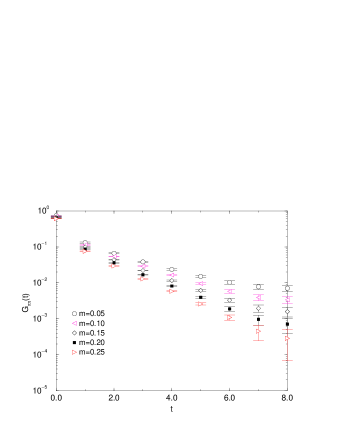
Figure 6: This figure shows the zero momentum correlation function $G_{\pi\pi}(t)$ as a function of time slice.

in order to extract the meson mass $\mu$. The kets $|x,t\rangle$ represent the normalized position basis states and the trace is over the spinor index. Using the eigenvalues and eigenstates of $D$ it is easy to evaluate the propagators necessary for the calculation of $G_{\pi\pi}(t)$. In figure (6) we plot it as a function of $t$. The function appears to fit to the usual form of $A\cosh(m(t-T/2))$, suggesting that conventional methods will be useful to extract the meson masses. A simple estimate of the meson mass can be made using the effective mass analysis. Defining the effective mass by

$$\mu_{\rm eff}(t)=-\log(G_{\pi\pi}(t)/G_{\pi\pi}(t-1)).$$ (14)

we plot the results in figure (7), which shows evidence for plateaux. We chose the values of $\mu_{\rm eff}$ at $t=5$ to estimate the meson mass. The meson masses are plotted in figure (8) as a function of the fermion mass. The continuum result in the Schwinger model, $\mu/g=1/\sqrt{\pi}$ is shown on the $m=0$ axis. Again our results agree with in the expected $10-15\%$ error margin. It is interesting to note that no factors of $Z$ are necessary here as this is a spectral quantity. However, the dependence of the meson mass on $M$ indicates a renormalization of the fermion mass and the coupling. This effect can be studied more concretely and is left for the future.

6. Discussion and Conclusions

We have reproduced the essential features of the Schwinger model rather easily on a coarse lattice using Neuberger’s formulation of Ginsparg-Wilson fermions. This was possible because the physics of the one flavor model is essentially governed by the topological sectors, which was reproduced quite well on a moderately coarse and finite lattice. We discovered an interesting connection between the zero modes and number of fermion flavors as a function of $M$. The value of $M$ was important in getting the right connection between the number of flavors and the zero modes of the Dirac operator. In the region $0>M>-2$, where the theory is expected to describe the right physics the dominant effect of $M$ in the chiral condensate was a wave-function renormalization. Evidence for the renormalization of the fermion mass and the coupling was also seen.

All this means that questions that are dominated by topological effects in QCD, such as the $\eta^{\prime}$ mass, may also be easily addressed with these fermions, once the right region in $M$ is isolated. Reproducing the physics of the anomaly has other interesting consequences. In particular it can help in a better understanding of the QCD phase transition. Most calculations in lattice QCD indicate a second order phase transition for two flavor QCD. The most reliable calculations come from staggered fermions which have a remnant chiral symmetry. However, we have seen that staggered fermions produce very weak anomalous effects. These results have been confirmed in QCD just above the phase transition [34]. As is well known [35], a very weak anomaly close to the transition can make the transition first order. Since this is not seen in simulations, our understanding of the two flavor transition may not be complete. On the other hand, since the Ginsparg-Wilson fermions reproduce the effects of the anomaly rather easily and in addition have the correct flavor structure, they may give a more definitive understanding of the chiral transition. First such results have been reported in the domain wall formulation [36]. The present study also indicates that the Ginsparg-Wilson fermions behave quite differently with respect to quenching: another feature of reproducing the zero mode physics well. Hence the effects of the fermion determinant will play a more interesting role in QCD and quenched singularities [28] could be easily seen with these fermions. This is perhaps the easiest to study, since it involves only quenched calculations.

One of the striking feature of QCD is the spontaneous breaking of chiral symmetry. Unfortunately this cannot be addressed in a two dimensional model due to the Mermin-Wagner theorem. On the other hand, there is very interesting physics associated with the many flavor Schwinger model. For example one expects a non-analytic dependence of the meson mass and the chiral condensate on the fermion mass [22]. As far as we know this has not been reproduced in the past mainly due to the lack of a good fermion formulation. We plan to extend the present calculation in that direction. However, since we cannot expect non-analytic behavior to emerge on a finite lattice, a more careful finite size scaling analysis would be necessary. Thus the many flavor Schwinger model will be considerably more difficult, but perhaps can serve as a useful guide for the study of chiral symmetry in QCD.

Acknowledgment

I would like to thank W. Bietenholz, T. Bhattacharya, T.-W. Chiu, N. Christ, R. Edwards, P. Hasenfratz, I. Hip, R. Mawhinney, R. Narayanan, F. Niedermayer, A. Smilga and P. Vranas for helpful discussions. As this article was about to be submitted I came to know of the work of T.-W. Chiu [37], who has also analyzed the role of $M$ discussed in this article. I also thank W. Bietenholz for his suggestions after a critical reading of the manuscript.

Figure 1: The geometric definition of the topological charge is compared with the index of the Dirac operator for 50 configurations generated at $\beta=0.5$ (top) $\beta=3.0$ (bottom).

Figure 2: This figure shows a histogram of the topological sectors generated at $\beta=3.0$ in the 2500 configurations that were analyzed.

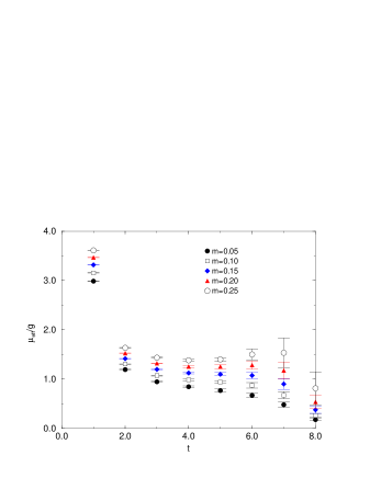
Figure 7: The effective meson mass at various time slices is plotted here to show evidence for plateaus.

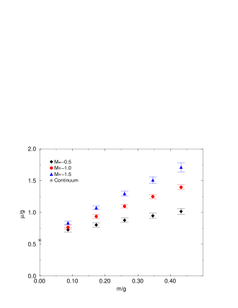
Figure 8: The meson mass is plotted as a function of the fermion mass for various values of $M$. The value in the continuum massless Schwinger model is represented by a star at $m/g=0$.

References

- [1] R. Narayanan and H. Neuberger, Nucl. Phys. B443 (1995) 305.
- [2] H. Neuberger, Phys. Lett. B417, (1997) 141.
- [3] M. Lüscher, Phys. Lett. B428 (1998) 342.
- [4] P. Ginsparg and K. Wilson, Phys. Rev. D25, (1982) 2649.
- [5] P. Hasenfratz, Nucl. Phys. B525 (1998) 401.
- [6] S. Chandrasekharan, hep-lat/9805015.
- [7] H. Neuberger, Phys. Lett. B427 (1998) 353.
- [8] P. Hasenfratz, Nucl Phys. B (Proc. Suppl.) 63 (1998) 53.
- [9] Y. Shamir, Nucl. Phys. B406 (1993), 90.
- [10] D. Kaplan, Phys. Lett. B288 (1992) 342.
- [11] H. Neuberger, Phys. Rev. D57 (1998) 5417.
- [12] T. Blum and A. Soni, Phys. Rev. D56 (1997) 174; Phys. Rev. Lett. 79 (1997) 3595.
- [13] P. Chen et.al., hep-lat/9807029.
- [14] F. Farchioni, C. B. Lang and M. Wohlgenannt, Phys.Lett. B433 (1998) 377.
- [15] F. Farchioni, I. Hip and C. B. Lang, hep-lat/9809016.
- [16] R. Narayanan, and P. Vranas, Nucl. Phys. B506 (1997) 373; Y. Kikukawa, H. Neuberger, Nucl. Phys. B(Proc. Suppl.)63 (1998) 590; Y. Kikukawa, R. Narayanan, and H. Neuberger Phys.Rev.D57 (1998) 1233.
- [17] P. Vranas, Phys. Rev. D57 (1998) 1415.
- [18] R. Narayanan, H. Neuberger and P. Vranas, Phys. Letts. B353 (1995) 507.
- [19] R. Narayanan, H. Neuberger and P. Vranas, Nucl. Phys. B(Proc. Suppl.) 47 (1996) 596;
- [20] I. Horváth, hep-lat/9808002.
- [21] P. Hernández, K. Jansen and M. Lüscher, hep-lat/9808010.
- [22] S. Coleman, Ann. Phys. 101 (1976) 239.
- [23] W. Bietenholz, hep-lat/9803023.
- [24] T.-W. Chiu, Phys. Rev. D58, (1998) 074511.
- [25] K. Jansen and M. Schmaltz, Phys. Lett. B296 (1992), 374.
- [26] Y. Shamir, hep-lat/9807012.
- [27] R. Narayanan and P. Vranas, Nucl. Phys. B506 (1997) 373; R. Edwards, U. Heller and R. Narayanan, hep-lat/9802016.
- [28] S. Sharpe, Phys. Rev. D46 (1992) 3146; C. Bernard and M. Golterman, Phys. Rev. D46 (1992) 853; R. Mawhinney, Nucl. Phys. B(Proc. Suppl.) 47 (1996) 557.
- [29] C. P. van den Doel, Nucl. Phys. B230 (1984), 250.
- [30] E. Marinari et. al., Nucl. Phys. B190 (1981) 734.
- [31] S. R. Carson and R. D. Kenway, Ann. of Phys. 166, (1986) 364.
- [32] A. Kaehler, hep-lat/9709141; Also see contribution to Lattice 98.
- [33] S. Chandrasekharan and N. Christ, Nucl. Phys. B(Proc. Suppl.) 47 (1996) 527;
- [34] N. Christ, Nucl. Phys. B(Proc. Suppl.) 53 (1997) 253; S. Chandrasekharan, et., al., hep-lat/9807018.
- [35] R. Pisarski and F. Wilczek, Phys. Rev. D29 (1984) 338.
- [36] P. Chen et. al., hep-lat/9809159
- [37] T.-W. Chiu, hep-lat/9810002.