A lattice potential investigation of quark mass and volume dependence of the $\Upsilon$ spectrum

Abstract

We investigate bottomonia splittings by solving a Schrödinger-Pauli-type equation with parametrisations of QCD potentials around those that have been determined previously in lattice simulations. This is done both, in the continuum and on finite lattices with resolutions ranging from $a=0.2$ fm down to $a=0.025$ fm and extent of up to 12 fm or $144^{3}$ lattice points. We find a strong dependence of some splittings, in particular the $2S-1S$ and $1P-1S$ splittings, on both the quark mass and the short range form of the static potential in the neighbourhood of the $b$ quark mass, while splittings such as $3S-2S$ and $2P-2S$ show reduced dependence on the short distance potential. We conclude that the quenched quarkonium spectrum cannot be matched to experiment with a simple redefinition of the lattice spacing. We investigate the size of relativistic corrections as a function of the quark mass. Finite size effects are shown to die out rather rapidly as the volume is increased, and we demonstrate the restoration of rotational symmetry as the continuum limit is taken.

I Introduction

Potential models have been applied to explain quarkonium spectroscopy [1] in cave paintings dating from the mesolithic era of QCD [2, 3, 4, 5, 6]. In the beginning, they were based on parametrisations of the potential [2, 3, 7] which were — at best — QCD motivated and subsequently fitted to the observed spectrum. During the past few years, however, a two-body Schrödinger-Pauli-type Hamiltonian incorporating the static potential and relativistic corrections due to spin dependent interactions as well as perturbations of the heavy quark propagator around the static Wilson line has been derived directly from the QCD Lagrangian to order $v^{4}$ in the heavy quark velocity [8, 9, 10, 11]. One-loop matching coefficients with renormalisation group running between terms within the effective Hamiltonian and QCD have been obtained [12, 11, 13, 14, 15]. Non-QCD input has still been required until all non-perturbative potentials have recently been determined from quenched lattice QCD by one of the present authors [11, 16]. Parametrisations have been fitted to these lattice potentials enabling Schrödinger-Pauli-type solutions to be formed that are genuine predictions of (quenched) QCD. The spectroscopy for quarkonia shows similar behaviour to that obtained using quenched NRQCD; however due to the use of a Hamiltonian formulation of the problem the potential approach allows the calculation of a wider range of states than it is possible within NRQCD, in a manner that is both accurate and more robust against finite size effects (FSE). Moreover, once the Hamiltonian is obtained, the quark mass can easily be varied.

We would like to mention that so far retardation effects have been neglected within the potential approach[17]. However, it appears likely that such effects, which have their origin in radiation of ultra-soft gluons, can be incorporated into the potential formulation in a rather elegant and straightforward manner [18] that should automatically account for spin exotic states and mixing between quark model and hybrid states [19]. This work indicates that — at least for the lowest lying bottomonium states in the quenched approximation — such effects are tiny, which explains the good agreement of our results with Lattice NRQCD predictions.

The obvious drawbacks of the potential approach are (a) that it cannot easily be extended to higher orders in the velocity where more and more non-potential type contributions will have to be included and (b) that — unlike HQET/NRQCD — it only applies to heavy-heavy systems. Bottomonia systems are the ideal application and — having access to all excited states — we are indeed provided with much more insight than if we were just able to calculate the lowest few excitations.

In this paper we shall investigate the major sources of error in lattice calculations of the bottomonium spectrum. For simplicity, we will only employ Cornell-type parametrisations of the potentials, neglecting a weakening of the effective QCD coupling at small quark separation. We study finite volume and discretisation effects by solving the order $v^{2}$ Hamiltonian on (three-dimensional) lattices, varying the physical volume and lattice spacing. Moreover, we study the size of relativistic and radiative corrections and estimate possible quenching effects by simulating the order $v^{2}$ and order $v^{4}$ Hamiltonians in the continuum, using parametrisations of the potentials that are motivated by fits to quenched lattice data [11]. We shall argue that, in order to reproduce the observed spectrum correctly, the unquenched potential must have a significantly stronger effective Coulomb coefficient at intermediate distances than determined within the quenched approximation, even when ignoring the weakening of this coefficient with the distance in the latter case.

The principal effect of this is that observable quantities which exhibit a large sensitivity to the short distance potential (e.g. states of small physical extent or fine splittings) will yield results that are inconsistent with those obtained from states that are more sensitive to physics at larger distances. These discrepancies will depend on the mean radius of the state in a manner that is far less benign than the naïve perturbative expectation of an enhanced slope of the logarithmic running of the coupling in the quenched approximation would suggest.

The paper is organised as follows. In Sec. II we present some simple theoretical expectations for the spin averaged spectrum and comment on results from Lattice spectroscopy investigations in view of these general considerations. In Sec. III we discuss the methods used for solving the Schrödinger-Pauli equation both in the continuum and using a discrete lattice formulation with boundary conditions imposing various cubic group representations to fix the orbital angular momentum, before we present our results in Sec. IV. We start with a discussion of systematic uncertainties imposed by truncating the expansion of the QCD Lagrangian at a given order in $v$ as well as due to radiative corrections to the matching coefficients of operators of dimension higher than four. Subsequently, results on the quarkonium spectrum as a function of the inverse quark mass with various effective Coulomb coefficients around those suggested by quenched and partially unquenched Lattice simulations are presented. The implications on the expected $n_{f}=3$, $m_{u}\approx m_{d}\approx 5$ MeV, $m_{s}\approx 100$ MeV Coulomb coefficient are discussed, and we rationalise both, the calculated mass dependence of the quenched $1P\,1S$ splitting and the analysis methods common in lattice heavy quark simulations. Finally, we proceed to a discussion of the dependence of the results on the lattice volume and spacing and characterise the likely finite volume errors and rotational symmetry restoration properties in the continuum limit of the lattice theory. In Sec. V, we summarise our results and present a brief outlook.

II General expectations

Naïvely one might expect that prior to a lattice simulation the lattice resolution $a$, at which the real world will be studied, is selected. In practice, however, the theory is non-dimensionalised and simulated at a given value of the bare coupling. Subsequently, the dimensionful lattice spacing is determined by matching an observable to its experimental value. If this observable depends on quark masses, the process of fixing the lattice scale cannot be disentangled from the problem of adjusting the quark masses, and simultaneous matching of two or more quantities to experiment has to be performed. It is therefore common to either choose a non-hadronic quantity, such as [20] $r_{0}$ (which is related to the static QCD potential) or to choose quantities defined at almost vanishing quark mass, such as $f_{\pi}$, to alleviate this problem. Despite the significant difference between the mass of a charm and a bottom quark, the spin averaged $1P\,1S$ splittings of the $\Upsilon$ and $J/\psi$ systems are found to be essentially the same in experiment. Therefore, it has been suggested that, in the above mentioned sense, this splitting was a particularly good quantity to set the lattice scale $a$ [21].

We note that in the potential picture the spin averaged splittings scale as $\Delta m\propto m^{-\frac{1}{3}}$ for a purely linear potential and as $\Delta m\propto m$ in the pure Coulomb case. For a logarithmic potential, the splittings are independent of the quark mass (see e.g. Ref. [5]). With a string tension $\kappa\approx 450$ MeV transition from one of these limits to the other sets in at a separation of order 0.5 fm, the static potential in the region $0.2$ fm$<r<1$ fm being approximately compatible with a logarithmic parametrisation, which provides an explanation of the similarity between the spin averaged charmonia and bottomonia level splittings.

It has been reported in quenched simulations, however, that the $1P\,1S$ splitting shows a significant slope as a function of [22, 23] $m_{\Upsilon}^{-1}$. Moreover, both the $2S\,1S$ and $1P\,1S$ splittings are found to be almost $20\%$ smaller than the experimental values if one sets the lattice spacing from light hadronic quantities [21, 24, 25, 26, 27] like $f_{\pi}$ or $m_{\rho}$ or the square root of the string tension 420 MeV$<\sqrt{\kappa}<$ 450 MeV, as determined from Reggé trajectories. Furthermore, calculations over a mass range extending above bottom have displayed a steep rise in the splittings [23] in the $m\rightarrow\infty$ limit, starting somewhat above the $b$ quark. From the potential picture, this can be explained as follows: as one increases the quark mass beyond the bottom mass, the states under consideration move deeper into the Coulomb region and splittings will diverge linearly in $m$, while in the limit of light quark masses splittings should grow like $m^{-1/3}$. This suggests that the beauty and charm masses lie within a broad minimum of the $1P\,1S$ and $2S\,1S$ splittings, the extent of experimental agreement largely being accidental. Of course in the limiting cases themselves, the potential picture will not be applicable: at light quark masses the description as a non-relativistic system breaks down while at extremely heavy quark masses, retardation effects will eventually dominate the dynamics [17].

It has been argued that the relevant physical momentum scales that affect bottomonia masses differ from those of light hadronic quantities. Neglecting sea quark loops in the quenched approximation alters the running of the QCD coupling, thereby resulting in large quenching errors when comparing quantities determined by different momentum scales [21, 26, 27, 28]. Indeed, in the presence of two light flavours of dynamical fermions the disagreement between mass ratios determined on the lattice and in experiment appears to be reduced [28, 26]. Some authors, therefore, suggest to adapt the lattice scale $a$ to the system under consideration in order to reduce quenching uncertainities [21].

The “different lattice spacings for different systems” argument obviously reduces the predictive power of quenched and partially unquenched simulations while it does not even work consistently within the $\Upsilon$ system: by integrating a Schrödinger-Pauli equation with quenched lattice potentials, the $\Upsilon$ $2S\,1S$ and $1P\,1S$ have been found [11] to be significantly smaller than one would have expected from the value of $am_{\rho}$. Deviations between experimental and quenched lattice ratios between $m_{\rho}$ and splittings incorporating larger radial states like $3S\,2S$ or $2P\,1P$, however, are found to be small [11, 29]. The first observation is in agreement with Lattice NRQCD results [21, 28]. Unfortunately, NRQCD precision results are only available for the $1S$, $1P$ and, to a lesser extent, $2S$ states, such that the above mentioned inconsistencies within the quenched $\Upsilon$ spectrum are largely hidden behind statistical errors and, possibly, FSE for $3S$ or $2P$ states.

We remark that the relevant exchange momentum will in general not only depend on the system but also on the state under consideration. One should also keep in mind that within the non-perturbative regime universality of the QCD $\beta$-function is lost. Therefore, interpreting differences between mass ratios determined within the quenched approximation and in full QCD as effects of an altered running of the strong coupling constant with one relevant scale is an overly simplistic picture. We conclude that neglection of sea quarks results in a scatter between different scale determinations of up to 20 %, a systematic uncertainty of the quenched approximation that cannot be repaired or discussed away.

Present day high precision data on the (partially) unquenched static QCD potential is limited to two light quarks with mass $m_{q}>25$ MeV. Apart from one very exploratory study [30], determinations of relativistic corrections for dynamical fermions are completely missing. Within statistical accuracy, data on the static potential obtained with two flavours of Wilson sea quarks as well as within the quenched approximation are compatible with the parametrisation, $V_{0}(r)=\kappa r-e/r$, down to distances as small as $0.2$ fm. From a fit to data with $r\geq r_{\min}=0.2$ fm one of the authors has obtained $e=0.292(5)$ in quenched simulations and $e=0.352(9)$ in the two flavour case with $m_{u}=m_{d}\approx 50$ MeV [29]. If we allow for an additional term, $f/r^{2}$, to mimic running coupling effects, we end up with $e\approx 0.32$ and $e\approx 0.37$, respectively. The latter fits incorporate the running of the Coulomb coefficient to distances $r\approx 0.1$ fm, significantly less than the mean radius of $\Upsilon(1S)$, $\langle r^{2}\rangle^{1/2}\approx 0.25$ fm, but only affect the parameter $e$ slightly, in comparison to the change induced by “switching on” two sea quarks. We conclude that the renormalisation of the effective intermediate distance Coulomb-coefficient is the dominant effect of unquenching, rather than the slightly different running of the coupling with the scale at large momenta.

For the sake of consistency with Ref. [11] we use the value $e=0.32$ throughout this article for what we call “quenched” while we estimate a value $e\approx 0.40$ for what we consider to be the real world with three flavours of light quarks. It is apparent from both, lattice data on the $1P\,1S$ splitting, and from the above information on the static potential that the Coulomb term is indeed underestimated in the quenched approximation. In what follows, we will investigate the dominant effect of unquenching by just varying the Coulomb coefficient in a Cornell potential simulation.

III Method

Throughout this paper we only use the Cornell-type parametrisation of QCD potentials, and neglect running coupling effects which would weaken the interaction at short distance. This means that we are likely to (slightly) overestimate fine structure splittings while the effect on spin averaged splittings is small. Physical states with small spatial extent like the $1S$ state should be thought of as being shifted into the direction of the corresponding prediction at somewhat weaker Coulomb coupling. Within this model, we estimate the sizes of various systematic effects, allowing conclusions on the degree of accuracy of lattice predictions on the $\Upsilon$ system.

Quenching effects and the importance of relativistic corrections are studied by solving a continuum Schrödinger equation by use of the Numerov method. Like in Ref. [11], we start from the Hamiltonian,

$$H=2\left[m+\delta m(m)\right]+H_{0}+\delta H_{\mbox{kin}}+\delta H_{\mbox{SI}}+\delta H_{\mbox{SD}},$$ (1)

with

$$H_{0}=\frac{{\mathbf{p}}^{2}}{m}+\overline{V}(r),$$ (2)

where

$$\overline{V}(r)=V_{0}(r)-\frac{1}{4m^{2}}\left\{c_{D}(m)b-2\left[c_{D}(m)-\frac{1}{3}\right]\kappa\right\}\frac{1}{r}.$$ (3)

The parametrisation,

$$V_{0}(r)=\kappa r-\frac{e}{r},$$ (4)

corresponds to the static QCD potential, the additional terms of Eq. (3) giving rise to order $v^{4}$ corrections to the energy levels. After solving the unperturbed Schrödinger equation,

$$\left(H_{0}-E_{nl}\right)\psi_{nll_{z}}({\mathbf{x}})=0,\quad\psi_{nll_{z}}({\mathbf{x}})=\frac{u_{nl}(r)}{r}Y_{ll_{z}}(\theta,\phi),$$ (5)

the remaining order $v^{4}$ relativistic corrections are computed as perturbations. The kinetic correction reads as follows,

$$\delta H_{\mbox{kin}}=-\frac{p^{4}}{4m^{3}}.$$ (6)

For the spin independent corrections we obtain,

$$\delta H_{\mbox{SI}}=\frac{1}{2m^{2}}\left\{4\pi e\left[1+\frac{c_{D}(m)}{2}-d_{s}(m)\right]\delta^{3}(r)-\frac{2e}{r}p^{2}-\left(\frac{\kappa}{3r}-\frac{e}{r^{3}}\right)L^{2}\right\},$$ (7)

while the spin dependent correction terms read,

$$\delta H_{\mbox{SD}}(r) = \frac{1}{2m^{2}}\left\{\left[-\frac{\kappa}{r}+\frac{4c_{F}(m)(e-h)-e}{r^{3}}\right]{\mathbf{L}\cdot S}\right.$$ (8)

$$+ 6c_{F}^{2}(m)\frac{(e-h)}{r^{3}}T$$ (9)

$$+ \left.8\pi\left[2c_{F}^{2}(m)-d_{v}(m)\right](e-h)\delta^{3}(r)\frac{\mathbf{S}_{1}\cdot S_{2}}{3}\right\},$$ (10)

with

$$\frac{{\mathbf{S}_{1}\cdot S_{2}}}{3} = \frac{1}{6}\left[s(s+1)-\frac{3}{2}\right],$$ (11)

$$\mathbf{L}\cdot S = \frac{1}{2}\left[j(j+1)-l(l+1)-s(s+1)\right],$$ (12)

$$T=\frac{{\mathbf{x}\cdot S_{1}}{\mathbf{x}\cdot S_{2}}}{r^{2}}-\frac{\mathbf{S}_{1}\cdot S_{2}}{3} = -\frac{6({\mathbf{L}\cdot S})^{2}+3{\mathbf{L}\cdot S}-2s(s+1)l(l+1)}{6(2l-1)(2l+3)}.$$ (13)

In the present investigation, we choose to approximate the matching coefficients by their tree-level values, $c_{F}(m)=c_{D}(m)=1$ and $d_{s}(m)=d_{v}(m)=\delta m(m)=0$, as it is usually done in Lattice NRQCD simulations too. If the quark mass $m$ differs from the gluon momentum cut-off $\mu$ at which the potentials have been evaluated, radiative corrections have to be considered.

With relations, such as $\langle nll_{z}|f(r){\mathbf{p}}^{2}|nll_{z}\rangle=m\langle nll_{z}|f(r)[E_{nl}-\overline{V}(r)]|nll_{z}\rangle$, all perturbations can be reduced to functions of the expectation values $\langle r^{\alpha}\rangle$ with $\alpha=-4,\ldots,1$ and $4\pi\langle\delta^{3}(r)\rangle=|\psi(0)|^{2}$ and the unperturbed energy levels $E_{nl}$. We use the parameter values of Ref. [11],

$$r_{0}^{-1}=406\mbox{~{}MeV},\quad h=0.065,\quad b=3.81\kappa.$$ (14)

We can convert $r_{0}$, defined as the distance $r$ at which [20] $r^{2}dV(r)/dr=1.65$, into the string tension,

$$\kappa=\frac{1.65-e}{r_{0}^{2}}.$$ (15)

The above value of $r_{0}$ has been obtained by optimising the spectrum with respect to all experimentally observed bottomonium states. The advantage of this procedure over a matching of just the two lowest lying splittings is that this $r_{0}$ comes out to be in closer agreement with scales obtained from light hadronic observables, such as $m_{\rho}$ or $f_{\pi}$. $e$ is varied starting from the (quenched) value $e=0.32$ in order to estimate sea quark effects while $m$ is varied between 1 and 15 GeV for investigation of the mass dependence of splittings. The values of $m$ that optimally reproduce the bottomonium and charmonium levels (within the quenched set-up) have been found to be $m_{b}\approx 4.68$ GeV and $m_{c}\approx 1.33$ GeV, respectively. An increase of $e$ by 25 % results in an increase of these mass estimates by only 1 % and 4 %, respectively.

We expect electromagnetic interactions to yield an increase of the parameter $e$ by $(1/3)^{2}\alpha_{f}(m_{b})\approx 10^{-3}$ for $\Upsilon$ states and $(2/3)^{2}\alpha_{f}(m_{c})\approx 3.5\times 10^{-3}$ for $J/\psi$ states. thereby having a negligible impact on the spectrum. $\alpha_{f}$ denotes the QED fine structure constant. The change results in an increase of about 2 MeV for a QCD prediction of $m_{b}$ and of about 8 MeV for $m_{c}$.

We estimate FSE for the $\Upsilon$ system by numerically solving the Schrödinger equation on three-dimensional cubic lattices. For this purpose, we work at order $v^{2}$ only and employ the following definition of the lattice Laplacian,

$$\nabla^{2}\psi({\mathbf{x}})=\frac{1}{a^{2}}\sum_{j=1}^{3}\left[\psi({\mathbf{x}}+a{\mathbf{e}}_{j})+\psi({\mathbf{x}}-a{\mathbf{e}}_{j})-2\psi({\mathbf{x}})\right],$$ (16)

which is correct up to order $a^{2}$ lattice artifacts (${\mathbf{e}}_{j}$ denotes a unit vector in direction $j$). Note that — to this order in $v$ — we use the standard Schrödinger equation,

$$\left[\frac{p^{2}}{m}+V_{0}(r)-E_{n}\right]\psi_{n}({\mathbf{x}})=0,$$ (17)

with the static potential $V_{0}(r)$ of Eq. (4) only, instead of $\overline{V}(r)$ of Eq. (3). $n$ is to be understood as a multi-index that completely characterises a given state. We choose the coordinate system such that the origin is in the centre of an elementary cube, therefore avoiding problems with the divergence of $V_{0}(r)$ at $r=0$. Throughout the simulations the parameters of Ref. [11] are used:

$$\sqrt{\kappa}=468\mbox{~{}MeV},\quad e=0.32,\quad m=4.676\mbox{~{}GeV}.$$ (18)

The discretised Hamiltonian is solved by use of a successive over-relaxation algorithm. Excitations are accessed via Gram-Schmidt orthogonalisation with respect to previously obtained solutions. Only one octant needs to be simulated, and different orbital states are generated by enforcing combinations of periodic (even) or anti-periodic (odd) boundary conditions along various lattice directions. We use the $z$-axis as our quantisation axis. Thus, we always apply the same boundary conditions along the $x$- and $y$-directions, such that four different combinations are realised: even $x$, even $z$ ($ee$); even $x$, odd $z$ ($eo$); odd $x$, even $z$ ($oe$); odd $x$, odd $z$ ($oo$). All other solutions can be obtained as linear superpositions of the solutions obtained in this manner with eventually permuted lattice axes.

For a cubic lattice the relevant discrete symmetry group is $O_{h}$. States can be classified in accord to the five irreducible representations $A_{1}$, $A_{2}$, $E$, $T_{1}$ and $T_{2}$. $A_{1}$ and $A_{2}$ are one-dimensional, $E$ is two-dimensional and $T_{1}$ and $T_{2}$ both are three-dimensional. The implemented boundary conditions determine the symmetry of the wave function under reflections with respect to a lattice plane through the origin. While this suffices to unambiguously single out $T_{1}$ ($eo$), $T_{2}$ ($oe$) and $A_{2}$ ($oo$) states, both $A_{1}$ and $E$ states fall into the same $ee$ class.

Each $O_{h}$ state has overlap to various continuum states with different angular momenta. In order to allow for an identification of the continuum spin content, the expectation value $\langle L^{2}\rangle=l(l+1)$ has been traced. Moreover, lattice spacing and volume have been changed and continuum and infinite volume extrapolations performed. In Table I, we have listed which states we expect to find within each set of boundary conditions. $S$ waves can only be found with $ee$ boundary conditions and $P$ waves only with $eo$ boundaries. In the latter case, with antiperiodic boundaries in the $z$-direction, we will only obtain the $l_{z}=0$ state. $D$ waves will be generated with both, $ee$ boundaries (two states, corresponding to $l_{z}=\pm 2$) and with $oe$ boundaries (three states of which only the $l_{z}=0$ state is possible with odd boundary conditions in the $z$ direction). Finally, $F$ waves will be obtained in the $eo$ and $oe$ (three states in each sector, of which we will only find one in either case) as well as in the $oo$ (one state) sectors.

Lattices with octants of up to $72^{3}$ sites are being realised and lattice spacings down to $a=0.025$ fm are simulated, enabling us to study both, finite volume effects and the restoration of rotational symmetry between different lattice representations with overlap to the same continuum angular momentum.

IV Results

A Relativistic and radiative corrections

We intend to estimate the uncertainties on spin averaged order $v^{4}$ NRQCD level splitting predictions, due to higher order corrections. For this purpose, in Fig. 1, we have plotted the average velocity $\langle nl|v^{2}|nl\rangle$ for various states as a function of the inverse quarkonium ground state mass, $M_{\Upsilon}^{-1}$. The vertical lines correspond to bottomonium and charmonium. For bottomonia states, we typically find $\langle v^{2}\rangle\approx 0.1$ while for charmonia we obtain $\langle v^{2}\rangle\approx 0.4$. Two sources of uncertainties that are common to both, the potential approach and Lattice NRQCD, exist: (a) radiative corrections to the coefficients of the NRQCD Lagrangian and (b) higher order relativistic corrections. Note that for the moment being our estimates apply to an exact prediction from order $v^{4}$ NRQCD with tree-level matching coefficients. We ignore errors that are due to the lattice discretisation or an inadequate representation of the potentials at short distance by the parametrisation used. In particular for $S$ wave and, to a lesser extent, $P$ wave fine structure splittings we expect such effects to be another significant source of uncertainty.

If we start from the non-relativistic result for a mass splitting, $\Delta M_{v^{2}}$, calculated at order $v^{2}$, the correct relativistic splitting can be obtained as an expansion in powers of the typical heavy quark velocity $v^{2}$,

$$\Delta M=\Delta M_{v^{2}}\left(1+c_{1}v^{2}+c_{2}v^{4}+\cdots\right).$$ (19)

We find values $c_{1}v^{2}=0.034(0.036)$ for the $\overline{2S}\,\overline{1S}$ and $c_{1}v^{2}=0.025(0.029)$ for the $\overline{1P}-\overline{1S}$ bottomonium splittings. The first numbers refer to the quenched estimate ($e=0.32$) while the numbers in brackets refer to $e=0.40$. The overline symbol denotes arithmetic averaging of all masses of states with the given quantum numbers; apparently, the sizes of the correction terms only weakly depend on quenching. For the $J/\psi$ system, we obtain the values $0.103(0.115)$ and $0.070(0.082)$, respectively. Thus, in both cases we find, $c_{1}\approx 1/3$.

We have set all coefficients of the NRQCD Lagrangian to their tree-level values. However, when matching the effective theory to QCD, radiative corrections come into play. As long as we are only concerned with the spin averaged spectrum, $\delta H_{\mbox{SD}}$ [Eq. (9)] does not contribute. Therefore, the only uncertainties enter in the terms of Eqs. (3) and (7) that contain the coefficient $c_{D}(m)$. Discarding these terms results in a shift of the $\overline{2S}\,\overline{1S}$ splitting of 5 MeV and 16 MeV in the $\overline{1P}\,\overline{1S}$ splitting for bottomonia and 2 MeV and 16 MeV for charmonia states, respectively. Based on the one-loop results of Refs. [13, 14], we estimate the uncertainty in $c_{D}$ to be as big as 25 % for $\Upsilon$ states and 100 % for $J/\psi$ states for simulations on lattices with resolutions $a\approx 0.08$ fm.

By assuming $c_{2}<c_{1}$, which is motivated by the observation that $c_{1}\approx 1/3<c_{0}=1$, we expect the order $v^{6}$ correction to be smaller than 2 MeV and 1.3 MeV for bottomonia $\overline{2S}\,\overline{1S}$ and $\overline{1P}\,\overline{1S}$ splittings, respectively. In case of charmonia, we can only roughly estimate the corresponding values to be 45 MeV and 20 MeV. Taking the additional uncertainty in $c_{1}$ due to radiative corrections to $c_{D}$ into account, we expect to be accurate within 5–6 MeV for $\Upsilon$ $\overline{1P}\,\overline{1S}$ and 3–4 MeV for $\overline{2S}\,\overline{1S}$ splittings which corresponds to a relative precision of about 1 %, while of the $J/\psi$ system we estimate 50 MeV and 40 MeV, respectively, which amounts to an expected accuracy of only 10 %.

Unfortunately, the singlet $S$ states for the $\Upsilon$ system have not been discovered in experiment yet. The triplet levels are increased by 10(12) MeV and 6.5(7.5) MeV in respect to the corresponding spin-averaged results, obtained at $e=0.32(0.40)$, for $1S$ and $2S$ states, respectively. By allowing an uncertainty of 25 % on the matching coefficient within Eq. (9), we estimate cumulated uncertainties of about 8–9 MeV and 5–6 MeV for bottomonium $\overline{1P}1^{3}S_{1}$ and $2^{3}S_{1}1^{3}S_{1}$ splittings, respectively. Note that a further uncertainty of up to 10 MeV has to be added to lattice results on the $1^{3}S_{1}$ state obtained around $a\approx 0.08$ fm to account for discretisation errors of the wave function at the origin [36].

The uncertainty in the $P$ wave fine structure, which by itself is an order $v^{4}$ effect, is much bigger of course. One might hope — again by assuming $c_{3}<c_{2}$ — that relativistic corrections are suppressed by a factor of order $v^{2}$ in respect to the leading order result. This alone would imply an uncertainty of 10 % for the bottomonium and 40 % for the charmonium fine structure. The uncertainty in radiative corrections is dominated by the error of $c_{F}^{2}(m)$, which, based on the two-loop calculation of Ref. [32], we expect to be about 25 % for bottom quarks and 70 % for charm quarks. In linearly adding these two sources of error, we end up with relative precisions of 35 % and 110 % for order $v^{4}$ $\Upsilon$ and $J/\psi$ fine structure splitting predictions, respectively, i.e. the predictive power for the charmonium fine structure is zero. However, meaningful results can still be obtained for ratios of fine structure splittings since these turn out to be (almost) independent of the matching coefficients.

B Mass dependence and quenching effects

As has been argued above, when the quark mass is increased quarkonia states move deeper into the Coulomb region and, with $m$ being the only remaining dimensionful parameter, all splittings will eventually diverge linearly with the quark mass. This can be seen from Fig. 2 where we compare the $2S\,1S$ splitting (calculated at order $v^{2}$) at a quark mass $m=5$ GeV with that at $m=15$ GeV. Of course, this also means that harder and harder gluons will obtain momenta lower than the (diverging) ultra-soft scale, $mv^{2}$, and the potential approach will loose validity, due to significant retardation effects. If we ignore this problem for the moment being, for very heavy quark mass we would expect the $2S\,1S$ and $1P\,1S$ splittings to become degenerate and diverge like,

$$M(2S)-M(1S)=\frac{3}{16}e^{2}m.$$ (20)

The situation is visualised in Fig. 3 for the unquenched case. The dotted curve is the expectation for a pure Coulomb potential which will asymptotically be approached by the two other curves as $m$ is increased. Around the bottom quark mass this pure Coulomb contribution amounts to about 20 % of the splittings while for the charm quark mass it contributes only slightly more than 5 %. A similar divergent behaviour is expected to set in for the $3S\,1S$ and $2P\,1S$ splittings at somewhat bigger quark masses.

In Fig. 4, we display the dependence of the ratio,

$$R=\frac{M(2^{3}S_{1})-M(1^{3}S_{1})}{M(\overline{1^{3}P})-M(1^{3}S_{1})},$$ (21)

on the inverse quarkonium ground state mass for various values of the Coulomb strength. For this purpose, we operate at fixed $r_{0}=406$ MeV [Eq. (14)] and adjust the string tension in accord with Eq. (15). The upper curves correspond to the order $v^{2}$ results, the lower curves to the order $v^{4}$ predictions. The Figure suggests a value $e\approx 0.40$ for real world QCD, which is somewhat larger than the $n_{f}=2$, $m_{u}=m_{d}\approx 50$ MeV upper limit $e=0.37(1)$ from a fit to a parametrisation that incorporates an $f/r^{2}$ term. Given the observed quark mass and flavour dependence [29, 37], the value $e\approx 0.40$ appears to be very reasonable. Within the systematic uncertainties discussed above, the experimental value of $R$ for the $J/\psi$ system is compatible with this choice of $e$ too. We obtain a quenched ($e=0.32$) bottomonium estimate, $R\approx 1.38$ which, while agreeing with Lattice NRQCD results [24], disagrees with experiment. The failure of the quenched potential to reproduce the observed $\Upsilon$ spectrum has also been noticed in Ref. [38].

In Fig. 5, we display the splittings between the $1^{3}S_{1}$ $\Upsilon$ ground state and $2^{3}S_{1}$ and $3^{3}S_{1}$ states (solid curves) as well as $\overline{1^{3}P}$ and $\overline{2^{3}P}$ states (dashed curves) for three values of the Coulomb coefficient, calculated to order $v^{4}$. All splittings decrease slightly with increasing quarkonium mass until they reach a turning point, after which they start to diverge. The position of this point critically depends on the level; for physically larger states it is shifted towards higher masses. It also depends on the strength of the Coulomb coefficient which explains why $R$ reacts in a very sensitive way towards quenching. While most level differences can be reasonably well reproduced with values $0.40\leq e\leq 0.45$, all splittings with respect to $1^{3}S_{1}$ are considerably underestimated, an effect that cannot be absorbed into redefinitions of the quark mass $m_{b}$ and the scale $r_{0}$ alone. We also note that differences between excitations and the $2^{3}S_{1}$ or $\overline{1P}$ levels exhibit a reduced dependence on $e$, compared to the splittings with respect to the physically smaller $1^{3}S_{1}$ state that are displayed in the figure.

By incorporating a weakening of the QCD coupling at shorter distance into the parametrisation of the interaction potential [39], the prediction can be brought in line with experiment within the estimated uncertainties of Sec. IV A. The $1S$ state turns out to be most sensitive towards the running of the coupling. In quenched Lattice NRQCD simulations [24], after adjusting the scale from the $2^{3}S_{1}1^{3}S_{1}$ and $\overline{1P}\,1^{3}S_{1}$ splittings, all other level spacings have been found to be overestimated, and this despite the fact that our study of FSE suggests that the NRQCD $3^{3}S_{1}$ mass is underestimated by up to 50 MeV on the finite simulation volume. The potential results suggest that the disagreement within the $\Upsilon$ spectrum as well as between determinations of the lattice spacing from light hadronic quantities and quarkonia level splittings will indeed be reduced in unquenched simulations. A determination of the minimal lattice resolution required to resolve the running of the QCD coupling sufficiently well for a precision determination of $\Upsilon$ levels is the subject of an ongoing study [36].

In Fig. 6, we investigate the $1^{3}P_{2}\,1^{3}P_{0}$ (solid curves) and $1^{3}P_{1}\,1^{3}P_{0}$ (dashed curves) fine splittings as a function of the inverse $\Upsilon$ mass for three values of the Coulomb coefficient. For $e=0.40$, we underestimate experiment by a factor of almost two. If we had included a running coupling into our parametrisation, the predicted splittings might have been even somewhat smaller. For lattice spacings 0.067 fm$<a<0.092$ fm, by assuming (somewhat arbitrarily) an ${\overline{MS}}$-scheme gluon momentum cut-off $\mu=\pi/a$, we obtain a one-loop estimate $1.06<c_{F}^{2}(m)<1.13$ [11], a range far away from the required 80–90 % correction. This result indicates, if we accept the conjecture that the spectrum should be described by QCD, that higher order contributions to the matching coefficients are important. As expected, predictive power of the potential approach (and Lattice NRQCD) on the fine structure is indeed limited by a huge systematic uncertainty. Note that the difference has nothing to do with uncertainties in “tadpole” factors since a non-perturbative renormalisation of lattice results with respect to the continuum is included into the parametrisations published in Ref. [11]. We expect to be accurate within 10 % for ratios of fine structure splittings, though. Indeed, the ratio of the two splittings at $e=0.40$ comes out to be $\rho\approx 1.56$, compared to the experimental value $\rho=1.66$.

C Finite size effects

In this Section, we will investigate FSE on the spin averaged spectrum for the quenched case. For this purpose, we restrict ourselves to the order $v^{2}$ Hamiltonian. In Fig. 7, we display the root mean squared radii of various wave functions for $e=0.32$ and $e=0.40$. Since the spatial extents of the states are apparently only weakly affected by the change in $e$, FSE in unquenched simulations are likely to behave in a very similar way, up to string breaking effects. FSE on the fine structure are expected to be negligible due to the short range nature of spin interactions. Note that all effects that we will discuss are entirely due to squeezing of the wave function and the presence of mirror charges on a torus. In lattice simulations additional sources of FSE in general exist and the behaviour of the quark propagator itself might be affected by the volume. Our prejudice, however, is that for heavy quarks such an effect can be neglected, as long as one remains comfortably separated from the deconfinement transition. This is definitely the case on volumes of $(1.5$ fm$)^{3}$.

In Fig. 8, we investigate the effect of a finite volume onto various splittings. The results have been obtained with lattice spacings $a=0.025,0.05,0.1$ and 0.2 fm and are extrapolated to the continuum limit. Note that on the cubic lattice, the $1D$ state exists in two representations, $1T_{2}$ and $1E$, that will only become degenerate in the infinite volume continuum limit. Obviously, the spectrum is very much affected by the box size for a lattice extent $L<1.5$ fm while for $L>2$ fm most levels have effectively approached their infinite volume limits. However, for the $3S$ level an extent as big as $2.5$ fm is required. Another representation of the data is displayed in Fig. 9 where we show $\delta M(L)=M(L)-M(\infty)$ as a function of $L$. In Table II we display the minimal lattice extents $L_{\mbox{3 MeV}}$ at which FSE were found to be smaller than 3 MeV for various states. For this purpose, the box size has been increased in steps of 0.05 fm. We have also included the root mean squared radii of Fig. 7. We find a linear behaviour, $L_{\mbox{3 MeV}}=a\langle r^{2}\rangle^{1/2}+b$ with $a\approx 2.25$ and $b\approx 0.65$ fm.

The finite size behaviour of the $1S$ level is well parameterised for $L>1$ fm by a polynomial in $L^{-3}$,

$$\delta M(L)=\sum_{i=1}^{4}\left(\frac{a_{i}}{L}\right)^{3i},$$ (22)

with

$$a_{1}=-0.088\mbox{~{}fm},\quad a_{2}=0.477\mbox{~{}fm},\quad a_{3}=-0.712\mbox{~{}fm},\quad a_{4}=0.717\mbox{~{}fm}.$$ (23)

The leading order coefficient is found to be rather small, compared to those of higher order correction, which is consistent with the fact that FSE set in rather suddenly. Parametrisations for other states are consistent with small coefficients of $L^{-3}$ terms too. While the finite size behaviour for $n=1$ states is monotonous, this is not the case for radial excitations anymore. In particular, the result for $3S$ (triangles) suggests that for some states infinite volume extrapolations of finite volume data might become dangerously non-trivial.

In Fig. 10 we display the $2P$ wave function, obtained on an $a=0.05$ fm lattice for various lattice extents, varying from 0.8 up to 2 fm. We show a cross section through the $x-z$ plane at $y=0$. Of course, the wave function vanishes within the plane $z=0$ and exhibits approximate rotational symmetry around the $z$-axis. From Fig. 9 one sees that the energy decreases up to 1.3 fm and increases again thereafter, until a second turning point is approached around 1.7 fm. From Fig. 10 we conclude that the second node of the wave function only fits onto the lattice for an extent slightly bigger than 1.2 fm, which explains the first turning point, while the second maximum of the wave function only starts to fit onto the lattice for $L>1.6$ fm, giving rise to the second turning point.

In Figs. 11 and 12 we display cross sections through the $1D$ wave function in the $E$ representation within the $x-z$ and $x-y$ planes, respectively. In Figs. 13 and 14, we show another $1D$ wave function in the $E$ representation. The energies of these two states are identically degenerate on all volumes. Finally, in Fig. 15, we display a $1D$ wave function in the $T_{2}$ representation. The wave function vanishes at $x=0$ and $y=0$. Interestingly, Fig. 15 looks very much like a rotated version of Fig. 11. On any finite lattice, we find the $1T_{2}$ energy level to differ from that of $1E$, even after the continuum extrapolation.

D Finite lattice spacing effects

We investigate the restoration of the continuum symmetry as the lattice spacing is reduced. We pay particular interest to states within different representations of the cubic symmetry group $O_{h}$ that are expected to contain the same $O(3)$ spin content. For instance, at a lattice spacing $a=0.1$ fm and infinite volume we find the $1T_{2}$ state to be by 4 MeV heavier than the $1E$ state. Unlike FSE, finite $a$ effects critically depend on the form of the action employed. With our discretisation of the Laplacian, we would expect order $a^{2}$ effects to leading order. Note that in our simulation, we have used a continuum parametrisation of the static QCD potential. In a lattice simulation, we would only obtain such a potential with a perfect gauge action. In general, one would expect the static potential to suffer under discretisation errors too. Insofar, the results stated here should be understood as mere lower limits on the discretisation errors of “real” lattice simulations of the $\Upsilon$ spectrum.

As an illustrative example, in Fig. 16, we display the spatial structure of the $3S$ state for various lattice spacings. While the general structure of the wave function is still quite well reproduced, even at $a=0.2$ fm, the peaks themselves are not very well sampled anymore. In Fig. 17 we extrapolate $S$ and $P$ states to the continuum limit. We observe that at finite lattice spacings all levels are somewhat underestimated — except for the $1S$ level which turns out to be slightly overestimated. Moreover, with increasing radial excitation $n$, the slope of the extrapolation in $a^{2}$ decreases. The lines have been obtained from fits to the $a=0.025$, 0.05 and 0.1 fm data points. This region is enlarged in Fig. 18.

We interpret the overestimation of the $1S$ level to be connected to the fact that we placed the origin — and therefore the singularity of the Coulomb potential — at the centre of an elementary lattice cube. As we increase the lattice spacing, the $S$ waves sample less and less of the potential around the singular region and, therefore, we underestimate this negative contribution to the total energy. The same argument holds had we taken a potential measured on the lattice, instead of the continuum parametrisation, since in this case the singularity would have been naturally cut off by the lattice spacing too. The decrease of the slope of the extrapolation with increasing number of nodes of the wave function can be explained by an underestimation of the kinetic energy due to the reduced curvature on a coarse lattice.

In Fig. 19, we investigate how degeneracies of different representations of $O_{h}$ that correspond to the same $O(3)$ spin content become restored in the continuum limit for $1D$ and $1F$ states. The $D$ state in the $T_{2}$ representation suffers less under both, finite $a$ effects and FSE than that in the $E$ representation. This is possibly due to the less complex structure of the wave function (Fig. 15). We observe the same for $F$ wave functions in the $A_{2}$ representation. While all states are in nice agreement with the leading order $a^{2}$ expectation up to a resolution $a=0.1$ fm, higher order terms have a considerable effect at $a=0.2$ fm. This is in particular so for the $1A_{2}$ state.

V Conclusions

We confirm that ratios of spin averaged bottomonium level splittings react in a sensitive way towards quenching. The main origin of this sensitivity is a renormalised overall-value of the intermediate energy effective QCD coupling, rather than an altered running of the coupling between different short distance scales. We find that the extent of agreement of spin averaged $2S\,1S$ and $1P\,1S$ splittings between the $\Upsilon$ and $J/\psi$ systems is somewhat accidental. Around the mass of the charm quark the slope of these splittings as a function of the inverse quark mass is quite significant but compensated for by a divergent term that gains influence within the region of the bottom quark mass.

We have estimated systematic uncertainties of calculations of quarkonia level splittings based on order $v^{4}$ NRQCD due to ${\mathcal{O}}(\alpha_{s}v^{4},v^{6})$ correction terms. We end up with estimated accuracies of 1–2 % and 10 % on spin averaged $\Upsilon$ and $J/\psi$ level splittings, respectively. For the fine structure, our estimates are 35 % and a factor two, respectively. The main sources of uncertainty in all cases are radiative corrections to the matching coefficients of dimension five and six operators within the effective Lagrangian, rather than higher order relativistic effects. Unless non-perturbative matching methods become available, we have little control over the bottomonium fine structure. By incorporating existing one- and two-loop results the uncertainty can be somewhat reduced. However, a comparison of the predicted fine structure with experiment indicates that even higher order contributions are significant and likely to exceed our estimated effect of 25 %. A slow convergence of perturbation theory is indicated by a recent two-loop calculation of $c_{F}(m)$ too [32].

We investigated finite volume effects, which we expect to be smaller for quarkonia than for light mesons. Nonetheless, even for bottomonia, a linear lattice extent bigger than 2 fm is advisable, at least if one is interested in radial excitations, such as the $2P$ or $3S$ levels. Except for the $1S$ state, we failed to find simple parametrisations of the finite size behaviour of energy levels, based on superpositions of a power series in the inverse spatial volume, and contributions that are exponentially suppressed. A general result, however, is that the coefficients of terms proportional to $L^{-3}$ come out to be smaller than those that accompany higher order corrections, which results in a rapid reduction of FSE, once a critical volume has been by-passed. We regard this result as relevant for all mesonic physics on the lattice.

Finally, we investigated finite lattice spacing effects. A non-vanishing spacing $a$ is required in lattice simulations of effective field theories to provide an ultra violet cut-off for gluon momenta, which means that the continuum limit cannot be taken. An unwanted by-product of the lattice regularisation is the violation of the continuum rotational symmetry and dispersion relation. By parameterising the potential, obtained at finite lattice spacing, with a continuous rotationally symmetric curve and subsequently solving the Hamiltonian in the continuum as well as on discrete lattices, we have qualitatively investigated the finite $a$ behaviour. We find it worthwhile to simulate Lattice NRQCD — where one is confined to lattice spacings in the region of the inverse quark mass — with different gluonic and fermionic actions and in particular to realise $D$ waves in both possible representations of the cubic symmetry group to gain control over discretisation errors.

Solving the Schrödinger-Pauli equation with lattice potentials on finite volumes provides us with a powerful tool to predict finite size effects in lattice simulations and to optimise smearing functions. The next step will be to extend the method to heavy-light systems within a Bethe-Salpeter framework which is theoretically not as rigorously founded as the potential approach for quarkonia but should still yield very valuable information on finite size effects and wave functions, which can then be used in lattice spectroscopy or determination of decay matrix elements. Another extension is the inclusion of retardation effects and incorporation of a running coupling into the parametrisation. Work along these lines is in progress.

TABLE I.: Spin content of states.

boundary ($xz$)	$O_{h}$	$l$
$ee$	$A_{1}$, $E$	$0,2,4\ldots$
$eo$	$T_{1}$	$1,3,\ldots$
$oe$	$T_{2}$	$2,3,\ldots$
$oo$	$A_{2}$	$3,6,\ldots$

TABLE II.: Smallest lattice extents at which FSE are found to be smaller than 3 MeV.

state	$L_{\mbox{3~{}MeV}}/$fm	$\langle r^{2}\rangle^{1/2}/$fm
$1S$	1.25	0.25
$1P$	1.55	0.41
$2S$	1.85	0.52
$1D(T_{2})$	1.75	0.54
$1D(E)$	2.0	0.54
$2P$	2.1	0.65
$3S$	2.4	0.74
$3P$	2.55	0.85

FIG. 1.: Average quark velocities for various states versus the inverse $1^{3}S_{1}$ mass. Solid curves correspond to $e=0.32$, dashed curves to $e=0.40$.

FIG. 2.: $2S$ and $1S$ levels and wave functions in comparison with the inter-quark potential ($e=0.4$, $r_{0}^{-1}=406$ MeV) for two quark masses.

FIG. 3.: Spin averaged $2S\,1S$ and $1P\,1S$ splittings versus the inverse quark mass ($e=0.4$).

FIG. 4.: $R=\Delta M_{2S\,1S}/\Delta M_{1P\,1S}$ as a function of $M_{\Upsilon}^{-1}$ for various values of the Coulomb coupling. The upper curves correspond to the static potential, the lower ones incorporate relativistic corrections.

FIG. 5.: Order $v^{4}$ $2^{3}S_{1}1^{3}S_{1}$ and $3^{3}S_{1}1^{3}S_{1}$ splittings (solid curves) as well as $\overline{1P}1^{3}S_{1}$ and $\overline{2P}1^{3}S_{1}$ splittings (dashed curves) versus the inverse $\Upsilon$ mass for various values of the Coulomb coupling. The dashed horizontal and vertical lines denote the experimental values.

FIG. 6.: The $1^{3}P_{j}$ fine structure as a function of the inverse $\Upsilon$ mass for various values of the Coulomb coupling. Solid curves denote the difference $M(1^{3}P_{2})-M(1^{3}P_{0})$, dashed curves $M(1^{3}P_{1})-M(1^{3}P_{0})$. The dashed horizontal and vertical lines denote the experimental values.

FIG. 7.: Radius of wave functions versus the inverse $\Upsilon$ mass. Solid curves correspond to $e=0.32$, dashed curves to $e=0.40$.

FIG. 8.: $\Upsilon$ splittings as a function of the lattice extent $L$.

FIG. 9.: Difference between $\Upsilon$ levels and their corresponding infinite volume values as a function of the lattice extent $L$.

FIG. 10.: The $2P$ wave function at $y=0$ for various lattice volumes.

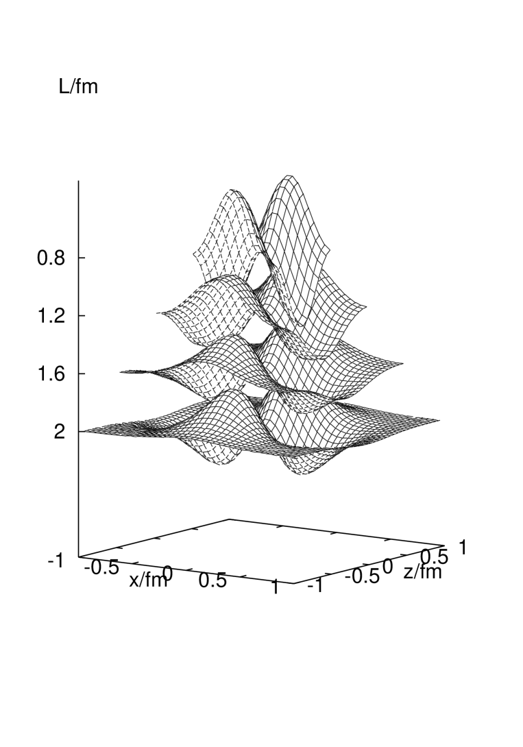
FIG. 11.: A $1D$ wave function in the $E$ representation at $y=0$ for various lattice volumes.

FIG. 12.: Same as Fig. 11 at $z=0$.

FIG. 13.: Another $1D$ wave function in the $E$ representation at $y=0$ for various lattice volumes.

FIG. 14.: Same as Fig. 13 for $z=0$.

FIG. 15.: A $1D$ wave function in the $T_{2}$ representation at $z=0$ for various lattice volumes. This wave function vanishes at $x=0$ and $y=0$, i.e. within the $x-z$ and $y-z$ planes.

FIG. 16.: The $3S$ wave function on lattices of extent $L=2$ fm and lattice spacings $a=0.025,0.05,0.1$ and 0.2 fm, respectively.

FIG. 17.: $S$ and $P$ states on lattices of extent 3.6 fm extrapolated to the continuum limit.

FIG. 18.: Same as Fig. 17.

FIG. 19.: $1D$ and $1F$ states within various lattice representations extrapolated to the continuum limit on a 3.6 fm lattice.