Sphaleron rate at high temperature in 1+1 dimensions

Abstract

We resolve the controversy in the high temperature behavior of the sphaleron rate in the abelian Higgs model in 1+1 dimensions. The $T^{2}$ behavior at intermediate lattice spacings is found to change into $T^{2/3}$ behavior in the continuum limit. The results are supported by analytic arguments that the classical approximation is good for this model.

Sphaleron physics plays an important role in theories of baryogenesis. A simple but useful model is the abelian Higgs model in 1+1 dimensions, given by

$$S = -\int{\rm d}^{2}x\;\left[\frac{1}{4g^{2}}F_{\mu\nu}F^{\mu\nu}+(D_{\mu}\phi)^{\ast}D^{\mu}\phi\right.$$

$$\left.\mbox{}+\mu^{2}|\phi|^{2}+\lambda|\phi|^{4}\right],$$

Recall that in 1+1 dimensions $\sqrt{\lambda}$ and $g$ have dimension of mass. A toy model for the electroweak theory is obtained by coupling to fermions, such that in the quantum theory the fermion current is anomalous. Changes in fermion number are then proportional to changes in Chern-Simons number

$$C=\frac{1}{2\pi}\int_{0}^{L}{\rm d}x_{1}\;A_{1},$$

thereby mimicking the B+L violation in the Standard Model. Here we assume space to be a circle of circumference $L$.

The sphaleron rate (of fermion number violation) $\Gamma$ can be identified from the diffusion of Chern-Simons number

$$\Gamma=\frac{1}{t}\left\langle\left[C(t)-C(0)\right]^{2}\right\rangle,\hskip 14.22636ptt\rightarrow\infty.$$

For relatively low temperatures this rate is exponentially suppressed by the sphaleron barrier. Numerical simulations [1, 2, 3] aggree with analytic results [4] in this regime. At high temperature the rate is not known analytically, but expected to be un-suppressed. For temperatures larger than any mass scale one may naively expect on dimensional grounds

$$\frac{\Gamma}{L}\propto T^{2}.$$ (1)

Such behavior was indeed found by us numerically and reported at LATTICE 94 [3]. However, De Forcrand, Krasnitz and Potting [1] gave a scaling argument that the behavior should instead be given by

$$\frac{\Gamma}{L}\propto T^{2/3}.$$ (2)

Figure 1: New data for $F=\Gamma/(m_{\phi}^{2}L)$ versus $T^{\prime 2}$ for the lattice spacings given in (4). The straight lines are fits to the data. The lower three lines do not fit the data very well.

This behavior (2) can also be argued for as follows. The simulations use the classical approximation

$$\langle[C(t)-C(0)]^{2}\rangle\approx\mbox{}$$

$$\frac{\int_{\varphi,\pi}e^{-H_{\rm eff}(\varphi,\pi)/T}\,\left[C(\varphi(t),\pi(t))-C(\varphi,\pi)\right]^{2}}{\int_{\varphi,\pi}e^{-H_{\rm eff}(\varphi,\pi)/T}}.$$

Here $\varphi$ and $\pi$ denote generic canonical variables and $\varphi(t)$ and $\pi(t)$ are solutions of the classical Hamilton equations with initial conditions $\varphi(0)=\varphi$, $\pi(0)=\pi$. The effective hamiltonian $H_{\rm eff}$ is approximated by its classical form. Rescaling $\varphi\to\varphi\sqrt{T}$, $\pi\to\pi\sqrt{T}$ produces $T$ only in the combination $\lambda T$ and $e^{2}T$. Since this combination has mass dimension three, the behavior (2) in the form $\Gamma/L\propto(\lambda T)^{2/3}$ appears natural.

We analyzed the quality of the classical approximation in perturbation theory and found the following favorable properties (in 1+1 dimensions!) [5]:

• Correlation functions of the basic fields are finite.

• The approximation becomes exact in the weak coupling/high temperature limit

  $$\lambda = v^{-2}|\bar{\mu}|^{2},\;\;\;g^{2}=\xi\lambda,\;\;\;T=v^{2}|\bar{\mu}|T^{\prime},\;\;\;$$

  $$v^{2} \to \infty,\;\;\;\xi,T^{\prime}\;\;\mbox{fixed}.$$ (3)

  Here $\bar{\mu}$ is the renormalized mass parameter in the $\overline{\mbox{MS}}$ scheme and $v^{2}=-\mu^{2}/\lambda$ is the classical ground state value of $2\varphi^{*}\varphi$. In the limit (3), $\mu^{2}/\bar{\mu}^{2}\to 1$. Notice that $T^{\prime}=\lambda T/|\bar{\mu}|^{3}$ involves the combination $\lambda T$.

In our previous results [3] the coefficient of $T^{2}$ appeared to vanish on extrapolation of the lattice distance to zero. At the time we interpreted this as an effect caused by using a too simple effective hamiltonian (the classical one), but now the perturbative analysis tells us that using the classical hamiltonian is fine in the limit (3). To settle the issue we carried out additional simulations at higher temperatures and smaller lattice spacings.

Fig. 1 shows the dimensionless rate

$$F\equiv\frac{\Gamma}{m_{\phi}^{2}L}$$

plotted versus $T^{\prime 2}$, for several lattice spacings,

$$a|\mu|=0.25,\;0.23,\;0.16,\;0.11,\;0.08.$$ (4)

There is clear $T^{2}$ behavior for the two larger spacings, but for the three smaller spacings this behavior does not fit the data any more. A crossover appears to take place between $a|\mu|=0.23$ and 0.16. In fact, $T^{2/3}$ behavior fits the data better at the three smaller spacings. Figs. 2–3 illustrate the behavior in more quantitative detail. Fitting the forms

$$F_{2} = c_{0}+c_{2}T^{\prime 2},$$

$$F_{2/3} = c_{0}+c_{2/3}T^{\prime 2/3},$$

led to

$$\chi_{2}^{2}/\mbox{d.o.f.} = 1.4,\;0.42,\;6.5,\;4.8,\;3.45,$$

$$\chi_{2/3}^{2}/\mbox{d.o.f.} = 28.9,\;21.6,\;2.5,\;1.1,\;1.2,$$

for $a|\mu|=0.25$, 0.23, 0.16, 0.11, 0.08, respectively. The volume was fixed at $|\mu|L=16$, and $\xi=4$.

Clearly, the $T^{2/3}$ form is favored for the three smaller lattice spacings. Extrapolating the resulting $c_{2/3}$ to zero lattice spacing, assuming a quadratic dependence on $a$ (cf. Fig. 2), gives the result $c_{2/3}=0.00452(86)$ for $a=0$, which translates into

$$\frac{\Gamma}{L}=0.0090(17)(\lambda T)^{2/3},\;\;\;g^{2}/\lambda=4.$$

Arguments for a $T^{2/3}$ behavior were given in ref. [1], where it was shown that the classical rate could be written in terms of a function $g(x,y)$, as $\Gamma/L=T^{2/3}g(a^{3}T,v^{3}/T)$, using units in which $\lambda=1$, suppressing $\xi$ dependence. For high temperatures $T^{2/3}$ behavior then followed in the continuum limit provided $g(0,0)\neq 0,\infty$ existed. For the case $v^{2}=0$, numerical data supported a nontrivial $g(0,0)$. Our analytic results [5] support the existence of a continuum limit of $g(a^{3}T,v^{3}/T)$, but notice how the combination $a^{3}T$ implies non-commutativity of the limits $a\to 0$ and $T\to\infty$. Unfortunately, our attempts to extrapolate first to zero lattice spacing failed because the resulting errors got too large. Our present analysis seems to indicate a behavior like $g(x,y)=g(0,0)+\beta(xy)^{2/3}+\alpha x^{4/3}+\gamma y^{4/3}+\cdots$, or $\Gamma/L=[g(0,0)+\beta a^{2}]T^{2/3}+\alpha a^{4}T^{2}+\gamma T^{-2/3}+\cdots$.

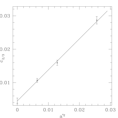
Figure 2: Plot of $c_{2/3}$ as a function of $a^{2}|\mu|^{2}$.

Figure 3: Top: data showing $T^{2/3}$ behavior for $a|\mu|=0.16$. Plotted is $F$ versus $T^{\prime 2/3}$ and a fit to $c_{0}+c_{2/3}T^{\prime 2/3}$. Bottom: same data plotted versus $T^{\prime 2}$. The straight line is a fit of $c_{0}+c_{2}T^{\prime 2}$. The curved line is the $T^{\prime 2/3}$ fit of the top figure. The data lack $T^{2}$ behavior but favor $T^{\prime 2/3}$ behavior in the region $a|\mu|\leq 0.16$.

References

• [1] P.Β de Forcrand, A.Β Krasnitz and R.Β Potting, Phys.Β Rev.Β D50 (1994) 6054.
• [2] J.Β Smit and W.H.Β Tang, Nucl.Β Phys.Β B (Proc.Β Suppl.) 34 (1994) 616.
• [3] J.Β Smit and W.H.Β Tang, Nucl.Β Phys.Β B (Proc.Β Suppl.) 42 (1995) 590.
• [4] A.I.Β Bochkarev and G.G.Β Tsitsishvili, Phys.Β Rev.Β  D40 (1989) 1378.
• [5] W.H.Β Tang and J.Β Smit, hep-lat/9805001.
Refer to caption