Dynamical Properties of Large $N$ Reduced Model of Yang-Mills Theory

Abstract

We study the large $N$ reduced model of $D$-dimensional Yang-Mills theory with special attention to the dynamical aspects related to the eigenvalues of the $N\times N$ matrices, which correspond to the space-time coordinates in the IIB matrix model. We define a quantity which represents the uncertainty of the space-time coordinates and show that it is of the same order as the extent of the space time, which means that the classical space-time picture is maximally broken. The absence of the SSB of the Lorentz invariance is also shown.

1 Introduction

Recently the large $N$ reduced models [1] have been revived in the context of nonperturbative formulations of string theory [2, 3]. The IIB matrix model [3, 4, 5], which is the reduced model of ten-dimensional supersymmetric Yang-Mills theory, is expected to be a nonperturbative formulation of superstring theory.

In this article, we study the large $N$ reduced model of Yang-Mills theory, which we refer to as the “bosonic model” in what follows. It is nothing but the bosonic part of the IIB matrix model. The action is given by

$$S=-\frac{1}{4g^{2}}\mbox{Tr}([A_{\mu},A_{\nu}]^{2}),$$ (1)

where $A_{\mu}$ $(\mu=1,\cdots,D)$ are $N\times N$ traceless hermitian matrices.

We investigate the dynamical aspects of the model related to the eigenvalues of $A_{\mu}$, which correspond to the space-time coordinates in the IIB matrix model. One of the most important quantities is the extent of the space time defined by $R=\sqrt{\langle\frac{1}{N}\mbox{Tr}(A^{2})\rangle}$. We also define a quantity which represents the uncertainty of the space-time coordinates and an order parameter for the SSB of the Lorentz invariance. We determine these values for the bosonic model by Monte Carlo simulation.

2 The extent of the space time

For $D$ $>$ 2 with sufficiently large $N$, the integral of $A_{\mu}$ is convergent without any cutoff because of an attractive potential between the eigenvalues of $A_{\mu}$ [6]. This enables us to absorb $g$ by rescaling $A^{\prime}_{\mu}=A_{\mu}/\sqrt{g}$ , which means that $g$ is nothing but a scale parameter. The large $N$ behavior of $R$ is, therefore, parametrized as $\sqrt{g}N^{\omega}$, since $R$ is proportional to $\sqrt{g}$ on dimensional grounds. In the IIB matrix model, $\omega$ plays an important role to deduce the space-time dimension, which is to be determined dynamically from the eigenvalue distibution of $A_{\mu}$ [7]. We determine $\omega$ for the bosonic model.

The observables we measure are the following.

$$(a) \left\langle\frac{1}{N}\mbox{Tr}(A^{2})\right\rangle\times\left(\sqrt{g}N^{1/4}\right)^{-2},$$

$$(b) \left\langle\frac{1}{N}\mbox{Tr}((A_{\mu}A_{\nu})^{2})\right\rangle\times\left(\sqrt{g}N^{1/4}\right)^{-4},$$

$$(c) \left\langle\frac{1}{N}\mbox{Tr}((A^{2})^{2})\right\rangle\times\left(\sqrt{g}N^{1/4}\right)^{-4},$$

$$(d) \left\langle\frac{1}{N}\mbox{Tr}(F^{2})\right\rangle\times\left(\sqrt{g}N^{1/4}\right)^{-4},$$ (2)

where $F_{\mu\nu}=i[A_{\mu},A_{\nu}]$. Here, we have normalized the above quantities so that they are dimensionless, and hence they are independent of $g$. We note that $(d)$ can be obtained analytically as $(d)=D(1-1/N^{2})$ [8].

In the Fig. 1, we show our results of Monte Carlo simulation for $D$ $=$ 4 with $N$ $=$ 4, 8, 16, 32, 64, 128, 256. One can see that $(a)$ $\sim$ $(d)$ are constant for $N\gtrsim 16$. In Fig. 2, we plot the data for $D$ $=$ 10 with $N$ $=$ 2, 4, 8, 16, 32. Here again we find that $(a)$ $\sim$ $(d)$ are constant for $N\gtrsim 16$.

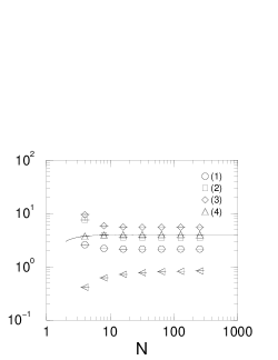
Figure 1: $(a)$ $\sim$ $(d)$ are plotted for $D=4$. The solid line represents the exact result for $(d)$. The tilted triangles are the plot of $\left\langle\Delta^{2}\right\rangle/(\sqrt{g}N^{1/4})^{2}$, which is discussed in Section 3.

Figure 2: $(a)$ $\sim$ $(d)$ are plotted for $D=10$. The solid line represents the exact result for $(d)$. The tilted triangles are the plot of $\left\langle\Delta^{2}\right\rangle/(\sqrt{g}N^{1/4})^{2}$, which is discussed in Section 3.

From these results, we find that $R$ is of the order of $O(\sqrt{g}N^{1/4})$, which means that the upper bound determined by the perturbative argument is saturated. The large $N$ behaviors of $(a)\sim(c)$ are consistent with the predictions from the perturbative expansion and the $1/D$ expansion of this model [8].

3 Breakdown of the classical space-time picture

In the IIB matrix model, the eigenvalues of $A_{\mu}$ represent the space-time coordinates. If $A_{\mu}$’s are commutable, they can be diagonalized simultaneously and the diagonal elements can be regarded as the classical space-time coordinates. Therefore it makes sense to ask to what extent the classical space-time picture is broken. To discuss this issue, we define a quantity which represents the uncertainty of the space-time coordinates.

We define such a quantity by the analogy to the quantum mechanics. We regard the matrices $A_{\mu}$’s as the linear operators which act on the linear space, which we identify as the space of states of particles. We take an orthonormal basis $|e_{i}\rangle$ ($i=1,2,\cdots,N$) and identify $|e_{i}\rangle$ with the state of the $i$-th particle. The space-time coordinate of the $i$-th particle is defined by $\langle e_{i}|A_{\mu}|e_{i}\rangle$. The uncertainty of the coordinate can be defined by

$$\delta(i)^{2}=\sum_{\mu}\left\{\langle e_{i}|A_{\mu}^{~{}2}|e_{i}\rangle-(\langle e_{i}|A_{\mu}|e_{i}\rangle)^{2}\right\}.$$ (3)

We take an average of $\delta(i)^{2}$ over all the particles and define the gauge-invariant quantity by

$$\Delta^{2}=\min_{\{|e_{i}\rangle\}}\left(\frac{1}{N}\sum_{i}\delta(i)^{2}\right).$$ (4)

Note that $\Delta=0$ if and only if $A_{\mu}$ are diagonalizable simultaneously.

We plot $\langle\Delta^{2}\rangle$ obtained by Monte Carlo simulation in Figs. 1 and 2. We find that $\langle\Delta^{2}\rangle/(\sqrt{g}N^{1/4})^{2}$ tends to a constant for large $N$. Thus we conclude that $\sqrt{\langle\Delta^{2}\rangle}$ is of the same order as $R$. If $\Delta$ were smaller than the typical distance between two particles, i.e., $\ell=RN^{-1/D}$, we might say that the classical space-time picture is good. Our result, however, shows that the classical space-time picture is maximally broken.

4 No SSB of Lorentz invariance

The SSB of Lorentz invariance is of paramount importance in the IIB matrix model, since if the space time is to be four-dimensional, the 10D Lorentz invariance of the model must be spontaneously broken.

The SSB of Lorentz invariance can be probed by

$$J=\frac{1}{D}I_{\mu\nu}I_{\mu\nu}-\left(\frac{1}{D}I_{\mu\mu}\right)^{2},$$ (5)

where $I_{\mu\nu}$ is defined by $I_{\mu\nu}=\mbox{Tr}(A_{\mu}A_{\nu})/N$. $J$ represents nothing but the variation of the eigenvalues of $I_{\mu\nu}$.

If $\langle J\rangle/R^{4}$ is nonzero in the large $N$ limit, the Lorentz invariance is spontaneously broken. Thus, $\langle J\rangle/(\sqrt{g}N^{1/4})^{4}$ can be considered as an order parameter of the SSB of Lorentz invariance. In Ref.[8], we show that when the large $N$ factorization holds, the order parameter goes to zero in the $N\rightarrow\infty$ limit. Indeed, we show that at all orders of the $1/D$ expansion, the factorization holds and the order parameter behaves as $1/N^{2}$.

In Fig. 3 we plot $\langle J\rangle/(\sqrt{g}N^{1/4})^{4}$ against $N$ for $D$ $=$ 4, 6, 8, 10. We see that the order parameter vanishes in the large $N$ limit, which means that the Lorentz invariance is not spontaneously broken. Note also that the large $N$ behavior of the order parameter can be nicely fitted to $1/N^{2}$. This is in accordance with the prediction by the $1/D$ expansion.

Figure 3: $\langle J\rangle/(\sqrt{g}N^{1/4})^{4}$ is plotted against $N$ for $D$ $=$ 4, 6, 8,10. The solid line represents the prediction for the $D\rightarrow\infty$ limit and the other lines represent the fit to the $1/N^{2}$ behavior [8].

5 Summary

We studied the dynamical aspects of the reduced model of bosonic Yang-Mills theory. We determined the extent of the space time and showed that the classical space-time picture is maximally broken. We also showed that Lorentz invariance is not spontaneously broken. We expect that our findings for the bosonic model provide a helpful comparison when we investigate the IIB matrix model.

References

- [1] T. Eguchi and H. Kawai, Phys. Rev. Lett. 48 (1982) 1063.
- [2] T. Banks, W. Fischler, S.H. Shenker and L. Susskind, Phys. Rev. D55 (1997) 5112.
- [3] N. Ishibashi, H. Kawai, Y. Kitazawa and A. Tsuchiya, Nucl. Phys. B498 (1997) 467.
- [4] M. Fukuma, H. Kawai, Y. Kitazawa and A. Tsuchiya, Nucl. Phys. B510 (1998) 158.
- [5] H. Aoki, S. Iso, H. Kawai, Y. Kitazawa and T. Tada, Prog. Theor. Phys. 99 (1998) 713.
- [6] W. Krauth and M. Staudacher, Phys. Lett. B435 (1998) 350, hep-th/9804119.
- [7] J. Nishimura and A. Tsuchiya, in progress.
- [8] T. Hotta, J. Nishimura and A. Tsuchiya, in preparation.