Grassmann integrals by machine

Abstract

I present a numerical algorithm for direct evaluation of multiple Grassmann integrals. The approach is exact and suffers no Fermion sign problems. Memory requirements grow exponentially with the interaction range and the transverse size of the system. Low dimensional systems of order a thousand Grassmann variables can be evaluated on a workstation.

In quantum field theory fermions are usually treated via integrals over anti-commuting Grassmann variables [2], providing an elegant framework for the formal establishment of Feynman perturbation theory. With non-perturbative approaches, such as Monte Carlo studies on the lattice, these objects are more problematic. Essentially all approaches formally integrate the fermionic fields in terms of determinants depending only on bosonic fields. When a background fermion density is present, as for baryon rich regions of heavy ion scattering, these determinants are not positive, making Monte Carlo evaluations tedious on any but the smallest systems[3]. This problem also appears in studies of many electron systems doped away from half filling.

Here I explore the possibility of directly evaluating the fermionic integrals, doing the necessary combinatorics on a computer[1]. This is inevitably a rather tedious task, with the expected effort growing exponentially with volume. Nevertheless, in the presence of the sign problem, all other known algorithms are also exponential. My main result is that this growth can be controlled to a transverse section of the system. I illustrate the technique with a low dimensional system involving of order a thousand Grassmann variables.

I begin with a set of anti-commuting Grassmann variables $\{\psi\}$, satisfying $\psi_{i}\psi_{j}+\psi_{j}\psi_{i}=0$. Integration is uniquely determined up to an overall normalization by requiring linearity and “translation” invariance $\int d\psi f(\psi+\psi^{\prime})=\int d\psi f(\psi)$. I normalize things so that

$$\int d\psi\ \psi=1\qquad\int d\psi\ 1=0.$$ (1)

Consider an arbitrary action $S(\psi)$ inserted into a path integral. I want to evaluate

$$Z=\int d\psi_{n}\ldots d\psi_{1}\ e^{S(\psi)}.$$ (2)

Formally this requires expanding the exponent and keeping all terms containing exactly one factor of each $\psi_{i}$.

I first reduce the required expansion into operator manipulations in a Fock space. Introduce a fermionic creation-annihilation pair for each fermionic field, $\psi_{i}\leftrightarrow\{a_{i}^{\dagger},a_{i}\}$. These satisfy the usual relations $[a_{i},a_{j}^{\dagger}]_{+}=\delta_{ij}.$ The space is built by applying creation operators to the vacuum, which satisfies $a_{i}{|0\rangle}=0$. It is convenient to introduce the completely occupied “full” state ${|F\rangle}\equiv a_{n}^{\dagger}...a_{2}^{\dagger}a_{1}^{\dagger}{|0\rangle}.$ Then I rewrite my basic path integral as the matrix element

$$Z\ =\ {\langle 0|}\ e^{S(a)}\ {|F\rangle}.$$ (3)

Expanding $e^{S}$, a non-vanishing contribution requires one factor of $a_{i}$ for each Fermion. This is the same rule as for Grassmann integration.

I now manipulate this expression towards a sequential evaluation. Select a single variable $\psi_{i}$ and define $S_{i}(a)$ as all terms from the action involving a factor of $a_{i}$. I define the complement $\tilde{S}_{i}$ as anything else, so that $S=S_{i}+\tilde{S}_{i}$. I assume a bosonic action so that $S_{i}$ and $\tilde{S}_{i}$ commute and $Z={\langle 0|}e^{\tilde{S}_{i}}e^{S_{i}}{|F\rangle}.$ Since $\tilde{S}_{i}$ contains no factors of $a_{i}$, the occupation number for that variable, $n_{i}=a_{i}^{\dagger}a_{i}$, vanishes between the two factors. I thus can insert a projection operator $1-n_{i}$

$$Z={\langle 0|}e^{\tilde{S}_{i}}\ (1-n_{i})\ e^{S_{i}}{|F\rangle}.$$ (4)

Since $1-n_{i}$ projects out an empty state at location $i$, I trivially have $a_{i}\ (1-n_{i})=0$. I can replace $\tilde{S}_{i}$ with the full action. Also, since $a_{i}^{2}=0$, the right hand factor expands as $e^{S_{i}}=1+S_{i}$, giving

$$Z={\langle 0|}e^{S}\ (1-n_{i})\ (1+S_{i}){|F\rangle}.$$ (5)

Repetition gives my main result

$$Z=\left\langle 0\left|\prod_{i}\left((1-n_{i})(1+S_{i})\right)\right|F\right\rangle.$$ (6)

assuming constants in the action are removed.

Eq. (6) summarizes the basic procedure. Create an associative array (hash table) to store general states of the Fock space. For a given state $|\psi\rangle=\sum_{s}\chi_{s}|s\rangle$ store the numbers $\chi_{s}$ labeled by $|s\rangle$. Initially this table only contains the one entry for the full state. The algorithm then loops over the Grassmann variables. For a given $\psi_{i}$, first apply $(1+S_{i})$ to the stored state. Then empty the location with the projector $1-n_{i}$. After all sites are integrated over, only the empty state survives, with the desired integral as its coefficient.

The advantages appear with a local interaction. All sites previously visited are empty, and involve no information. Unvisited locations outside the interaction range are still filled, and also involve no storage. All relevant states are nontrivial only for unvisited sites within range of previously visited sites. Sweeping through the system in a direction referred to as “longitudinal,” we only need keep track of a “transverse” slice of the model. This is illustrated in Fig. (1). Although the dimension of the Fock space is two to the number of Grassmann variables, the storage requirements only grow as two to the transverse volume.

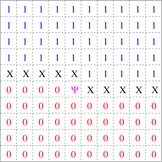
Figure 1: Integrating out sequentially, visited sites are empty and out of range sites are filled. When integrating the site labeled $\psi$, only those sites labeled “X” are undetermined.

The approach is exact, with no sign problems. The complexity grows severely with interaction range, probably limiting practical applications to short range interactions in low dimensions. Note that the effort only grows linearly with the longitudinal dimension, allowing very long systems. This discussion has been in the context of “real” Grassmann variables. For “complex” variables treat $\psi$ and $\psi^{*}$ independently.

In the transverse direction the boundary conditions are arbitrary, but longitudinal boundaries should not be periodic. To make them so requires maintaining information on both the top and bottom layers of the growing integration region, squaring the difficulty. Note that the technique is similar to the finite lattice method used for series expansions [4], and closely related to a direct enumeration of fermionic world lines [5].

As a test, consider a spin-less fermion hopping along a line of sites. I introduce a complex Grassmann variable on each site of a two dimensional lattice and study

$$Z=\int(d\psi d\psi^{*})e^{S_{t}+S_{h}+S_{I}}$$ (7)

with the various terms

$$\matrix{S_{t}=\sum_{i,t}\psi^{*}_{i,t}(\psi_{i,t}-\psi_{i,t-1})\hfill\cr S_{h}=k\sum_{i,t}\psi^{*}_{i,t}\psi_{i+1,t}+\psi^{*}_{i+1,t}\psi_{i,t}\hfill\cr S_{I}=g\sum_{i,t}\psi^{*}_{i,t}\psi_{i,t}\psi^{*}_{i+1,t}\psi_{i+1,t}.\hfill\cr}$$ (8)

I take $N_{t}$ sites in the time $t$ direction and $N_{i}$ spatial sites. The one-sided form of the temporal hopping insures an Hermitean temporal transfer matrix[6]. This model Bosonizes into an anisotropic quantum Heisenberg model, a fact not being used here.

I treat $t$ as my “transverse” coordinate, growing the lattice along the spatial chain. Fig. (2) shows the $N_{t}$ dependence for the free energy with $k=1$ and $g=\pm 1$. Here memory requirements were reduced by using time translation invariance after integrating each layer. The $N_{t}=14$ points were run on the RIKEN/BNL Supercomputer.

Figure 2: The free energy $F=\log(Z)/N_{i}N_{t}$ with a four fermion interaction as described in the text, plotted as a function of the number of time slices $N_{t}$. The chain has $N_{i}=50$ sites. Points are shown for $k=1$ and $g=\pm 1$.

With Monte Carlo methods, a chemical potential term can be highly problematic due to cancelations. Here, however, it is just another local interaction of negligible cost. As an illustration, take $S=S_{t}+S_{h}+S_{I}+S_{M}$ with

$$S_{M}=M\sum_{i,t}\psi^{*}_{i,t}\psi_{i,t}.$$ (9)

This regulates the “filling,” which can be approximately monitored as $(1+M){dF\over dM}$. I include the factor of $1+M$ to compensate partially for finite $N_{t}$ artifacts. Fig. (3) shows the filling as a function of $MN_{t}$ on an $N_{t}=8$ by $N_{i}=20$ lattice with a spatial hopping parameter of $k=0.1$. Here I made a crude extrapolation in chain length by defining $F={1\over N_{t}}\log\left({Z(N_{i})\over Z(N_{i}-1)}\right)$ . Note how the four fermion coupling enhances the filling.

Figure 3: The occupancy of a 20 site chain as a function of the chemical potential scaled by the number of time slices. The filling occurs earlier or later depending on the sign of the coupling.

An obvious system for future study is the Hubbard model[7]. This requires 4 Grassmann variables per site corresponding to $\psi^{*}$ and $\psi$ for spins up and down. Higher spatial dimensions strongly increase the size of the transverse volume and will limit practical system volumes, but this may be compensated for by the lack of sign problems.

References

- [1] M. Creutz, hep-lat/9806037 (1998).
- [2] F.A. Berezin, The method of second quantization, (Academic Press, NY, 1966).
- [3] I.M. Barbour and A.J. Bell, Nucl. Phys. B372, 385 (1992); I.M. Barbour, J.B. Kogut, and S.E. Morrison, Nucl. Phys. B (Proc. Suppl.) B53, 456 (1997).
- [4] Binder Physica 62 (1972) 508; T. de Neef and I.G. Enting, J. Phys. A10, (1977) 801; I.G. Enting, Aust. J. Phys. 31 (1978) 515; A.J. Guttmann and I.G. Enting, Nucl. Phys. B (Proc. Suppl.) 17 (1990) 328; G. Bhanot, M. Creutz, I. Horvath, J. Lacki, and J. Weckel, Phys. Rev. E49, 2445 (1994).
- [5] M. Creutz, Phys. Rev. B45, 4650 (1992).
- [6] M. Creutz, Phys. Rev. D35, 1460 (1987)
- [7] J. Hubbard, Proc. R. Soc. London A276, 283 (1963); A281, 401 (1964).