UNIGRAZ- UTP-03-09-98 Wilson, fixed point and Neuberger’s lattice Dirac operator for the
Schwinger model

Abstract

We perform a comparison between different lattice regularizations of the Dirac operator for massless fermions in the framework of the single and two flavor Schwinger model. We consider a) the Wilson-Dirac operator at the critical value of the hopping parameter; b) Neuberger’s overlap operator; c) the fixed point operator. We test chiral properties of the spectrum, dispersion relations and rotational invariance of the mesonic bound state propagators.

PACS: 11.15.Ha, 11.10.Kk
Key words: Lattice field theory, fixed point action, overlap operator, Dirac operator spectrum, zero-modes, topological charge, Schwinger model

1 Motivation and Introduction

The Nielsen-Ninomiya [1] theorem and the Ginsparg-Wilson [2] condition (GWC) provide us with the crucial information under which circumstances [3] remnants of chiral symmetry may stay with a lattice action for fermions, like it is e.g. the case for overlap fermions [4] or fixed point actions [5]. Recently Lüscher [6] has pointed out the explicit form of the underlying symmetry and indicated possible generalizations.

Fermion actions for massless fermions satisfying the GWC

$$\frac{1}{2}\left\{\,{\cal D},\gamma^{5}\,\right\}=a\,\left(\,{\cal D}\,\gamma^{5}\,R\,{\cal D}\,\right)\;\;,$$ (1)

where ${\cal D}$ is the lattice Dirac operator, violate chiral symmetry up to a local term ${\cal O}(a)$; the r.h.s. of the above equation is local since $R$ is.

It was pointed out in [3] that actions which are fixed points under real space renormalization group (block spin) transformations (BST), are solutions of the GWC. $R$ is then local and bounded and as a consequence the spectrum of ${\cal D}$ in complex space is confined between two circles [5]:

$$|\lambda-r_{min}|\geq r_{min}\;,\quad|\lambda-r_{max}|\leq r_{max}\;\;,$$ (2)

where the real numbers $r_{min}$ and $r_{max}$ are related to the maximum and minimum eigenvalue of $R$ respectively. For non-overlapping BSTs $R=\frac{1}{2}$ and (2) reduces to $|\lambda-1|=1$, i.e. the spectrum lies on circle.

Independent solutions of the GWC are provided by the overlap formalism [4], which allows the formulation of chiral fermions on the lattice. These solutions are obtained in an elegant way, as shown recently by Neuberger [7, 8], through some projection of the Wilson operator with negative fermion mass. Even in this case we have $R=\frac{1}{2}$ and $|\lambda-1|=1$.

For the Schwinger model (2D QED) we are in a situation where we have access to three different lattice Dirac operators for massless fermions, namely the original Wilson operator ${\cal D}_{\textrm{\scriptsize Wi}}\,$at $\kappa_{c}(\beta)$, the Neuberger-projected operator ${\cal D}_{\textrm{\scriptsize Ne}}\,$and a numerically determined and therefore approximate fixed point operator ${\cal D}_{\textrm{\scriptsize Fp}}\,$[9, 10]. Studying these alternatives we may ask the following questions:

• For given gauge field configurations: What is the relation between real eigenvalues of the lattice Dirac operator and the geometric topological charge? To what extent is the Atiyah-Singer Index Theorem (ASIT) realized in these lattice environments?

• In the continuum, the eigenvalue distribution is related to the condensate $\langle\bar{\psi}\psi\rangle{}$ (Banks-Casher formula [11]). What about the lattice theory for the given Dirac operators?

• The first two questions concern chiral symmetry and the phenomenon of fermion condensation. Important for the eventual study of the continuum limit of the full theory are also spectral properties: What is the behavior of e.g. dispersion relations? Concerning off-shell properties, what about recovery of rotational invariance of the propagators?

Here we perform a Monte Carlo simulation for the one- and two-flavor Schwinger model with gauge fields in the compact representation and the three different lattice Dirac operators. For the two-flavor model one expects a massless bound state in the chiral limit, which is of particular interest in this framework. We stress that the ensemble of gauge configurations used is the same in all three cases, the sampling being performed using the one-plaquette standard gauge action. The unquenching is obtained through the multiplication by the fermion determinant.

2 Lattice Dirac Operators

The three fermion actions may be written $\bar{\psi}\,{\cal D}\,\psi$, where the fields at each site are two-components Grassmann variables $\bar{\psi},\psi$ and ${\cal D}$ is a matrix in Euclidean and Dirac space (lattice Dirac operator). For two flavors the number of fields duplicate and the action becomes $\bar{u}\,{\cal D}\,u+\bar{d}\,{\cal D}\,d$ (with independent Grassmann fields $\bar{u}$, $u$, $\bar{d}$, $d$).

All three Dirac operators are non-hermitian but have $\gamma_{5}$-hermiticity:

$\gamma_{5}{\cal D}\gamma_{5}={\cal D}^{\dagger}$. Their eigenvalue spectrum is therefore symmetric with regard to complex conjugation.

2.1 Wilson Dirac operator

We write the Wilson Dirac operator in the form

$${\cal D}_{\textrm{\scriptsize Wi}}\,{}(x,y)=(m+D)\,\textrm{\boldmath{$\mathsf{1}$}}_{xy}-\frac{1}{2}\sum_{\mu}\left[(1+\sigma_{\mu})\,U_{xy}\,\delta_{x,y-\mu}+(1-\sigma_{\mu})\,U_{yx}^{\dagger}\,\delta_{x,y+\mu}\right]\;.$$ (3)

The hopping parameter $\kappa$ is related to the (bare) quark mass $m$ through the relation $\kappa=1/(2m+2D)$.

The chiral limit is obtained in this environment for $\kappa\rightarrow\kappa_{c}(\beta)$, where $\kappa_{c}(\beta)$ should be determined in some way (see the following). Thus we will work at $D=2$, and $\kappa=\kappa_{c}(\beta)$ (corresponding massless quarks) as discussed below.

2.2 Neuberger’s operator

Neuberger suggests [7] to start with the Wilson Dirac operator at some value of $m\in(-1,0)$ corresponding to $\frac{1}{2D}<\kappa<\frac{1}{2D-2}$ and then construct

$${\cal D}_{\textrm{\scriptsize Ne}}\,{}=\textrm{\boldmath{$\mathsf{1}$}}+\gamma_{5}\,\epsilon(\gamma_{5}\,{\cal D}_{\textrm{\scriptsize Wi}}\,{})\;.$$ (4)

We call the actual value of $\kappa$ used in the above definition $\kappa_{\textrm{\scriptsize Ne}}{}$. Some words about the choice of $\kappa_{\textrm{\scriptsize Ne}}{}$: according to [8] it is arbitrary, in the sense that any (strictly negative) value of $m$ in the interval $(-1,0)$ reproduces the correct continuum theory (see also the discussion on a suitable choice of $\kappa_{\textrm{\scriptsize Ne}}{}$ in [12]), but it may be optimized with regard to its scale dependence by looking for example at the behavior of the (projected) spectrum. Comparing expectation values of operators like $\langle\bar{\psi}\psi\rangle{}$ for different $\kappa_{\textrm{\scriptsize Ne}}{}$ one has to take care of the proper normalization [13]. One may see from the comparison with free lattice fermions that there is a (trivial) factor of $\sqrt{m}$, i.e. $\langle\bar{\psi}\psi\rangle{}=\langle\bar{\psi}\psi\rangle{}_{\textrm{\scriptsize Ne}}/|m|$ in our convention. Whenever not mentioned otherwise we choose $\kappa_{\textrm{\scriptsize Ne}}{}=\frac{1}{2}$ ($m=-1$) for our exploration; we also discuss results with some smaller values.

The operative definition of $\epsilon(\gamma_{5}\,{\cal D}_{\textrm{\scriptsize Wi}}\,{})$ entering the above equation is:

$$\epsilon(\gamma_{5}\,{\cal D}_{\textrm{\scriptsize Wi}}\,{})=U\,\textrm{Sign}(\Lambda)\,U^{\dagger}\quad\textrm{with}\;\gamma_{5}\,{\cal D}_{\textrm{\scriptsize Wi}}\,{}=U\,\Lambda\,U^{\dagger}\;.$$ (5)

Here $\textrm{Sign}(\Lambda)$ denotes the diagonal matrix containing the signs of the eigenvalue matrix $\Lambda$ obtained through the unitary transformation $U$ of the hermitian matrix $\gamma_{5}\,{\cal D}_{\textrm{\scriptsize Wi}}\,{}$. There are various efficient ways to numerically find ${\cal D}_{\textrm{\scriptsize Ne}}\,$without passing through the diagonalization problem, prohibitive for $D=4$ [14] (for $D=2$, see also [15]). In our simple context computer time is no real obstacle and therefore we use the direct definition (5), explicitly performing the diagonalization.

As observed in [8], gauge configurations with non-zero topological charge imply exact zero eigenvalues of ${\cal D}_{\textrm{\scriptsize Ne}}\,{}$. The subsequent inversion, necessary to find the quark propagators, is then not possible. The correct way to proceed is to introduce a regulator cutoff-mass: ${\cal D}\rightarrow{\cal D}+\mu\,\textrm{\boldmath{$\mathsf{1}$}}$ and then consider the limit $\mu\rightarrow 0$.

2.3 Fixed point Dirac operator

In [9] the fixed point Dirac operator was parameterized as

$${\cal D}_{\textrm{\scriptsize Fp}}\,{}(x,y)=\sum_{i=0}^{3}\sum_{x\,,f}\,\rho_{i}(f)\,\sigma_{i}\,U(x,f)\;,\quad\textrm{with}\;y\equiv x+\delta f\;.$$ (6)

Here $f$ denotes a closed loop through $x$ or a path from the lattice site $x$ to $y=x+\delta f$ (distance vector $\delta f$) and $U(x,f)$ is the parallel transporter along this path. The $\sigma_{i}$-matrices denote the Pauli matrices for $i=1,2,3$ and the unit matrix for $i=0$. The action obeys the usual symmetries as discussed in [9]; altogether it has 429 terms per site. The action was determined for gauge fields distributed according to the non-compact formulation with the Gaussian measure. There excellent scaling properties, rotational invariance and continuum-like dispersion relations were observed at various values of the gauge coupling $\beta$.

In [10] the action was studied both, for compact and the original non-compact gauge field distributions. In the compact case the action is not expected to exactly reproduce the fixed point of the corresponding BST, but nevertheless it is still a solution of the GWC; violations of the GWC are instead introduced by the parameterization procedure, which cuts off the less local couplings. We demonstrated that indeed the spectrum is close to circular, somewhat fuzzy at small values of $\beta\leq 2$ but excellently living up to the theoretical expectations of [5] at large gauge couplings $\beta\geq 4$.

Here we study the action only for the compact gauge field distributions in order to allow a direct comparison with the other lattice Dirac operators.

3 Simulation Details

Uncorrelated gauge configurations have been generated in the quenched setup. However, we are including the fermionic determinant in the observables: all the results presented here are obtained with the correct determinant (squared, for two flavors) weight. From earlier experience [9, 10] we know that this is justifiable for the presented statistics. We perform our investigation on three sets of 5000-10000 configurations at $\beta=2$, 4 and 6.

The so-called “geometric definition” of the topological charge is

$$Q_{G}=\frac{1}{2\pi}\,\sum_{x}\,{\rm Im\,ln}(U_{12}(x))\;;$$ (7)

we keep track of its value for all our configurations. The configurations have been well separated by $3\,\tau_{\textrm{\scriptsize int}}$, the autocorrelation length for $Q_{G}$.

For ${\cal D}_{\textrm{\scriptsize Wi}}\,$we need to determine $\kappa_{c}(\beta)$. We use PCAC techniques for this purpose [16] determining $\kappa_{c}$ for the unquenched 2-flavor case.

For each configuration we then build ${\cal D}_{\textrm{\scriptsize Wi}}\,$(at $\kappa_{c}(\beta)$), ${\cal D}_{\textrm{\scriptsize Ne}}\,$and ${\cal D}_{\textrm{\scriptsize Fp}}\,$as discussed. Each lattice Dirac matrix is diagonalized to obtain the complex eigenvalue spectrum. This is somewhat time-consuming due to the non-hermiticity. Furthermore the inverse (the quark propagator) is determined.

In the 2-flavor Schwinger model one expects [17] (for a recent discussion cf. [18]) one massive mode (called $\eta$ by analogy) and a massless flavor-triplet (called $\pi$). The corresponding momentum-projected operators are

$$\eta(p,t) = \sum_{x_{1}}\,e^{ipx_{1}}\left(\bar{u}(x_{1},t)\,\sigma_{1}\,u(x_{1},t)+\bar{d}(x_{1},t)\,\sigma_{1}\,d(x_{1},t)\right)\;,$$ (8)

$$\pi_{3}(p,t) = \sum_{x_{1}}\,e^{ipx_{1}}\left(\bar{u}(x_{1},t)\,\sigma_{1}\,u(x_{1},t)-\bar{d}(x_{1},t)\,\sigma_{1}\,d(x_{1},t)\right)\;.$$ (9)

Their correlation functions define by their exponential decay the corresponding energy functions $E(p)$ and thereby the dispersion relation. In the 1-flavor case only the massive mode is there.

We also study rotational symmetry via the correlation function

$$P(x)=\langle\bar{\psi}(0)\,\sigma_{3}\,\psi(0)\,\bar{\psi}(x)\,\sigma_{3}\,\psi(x)\rangle$$ (10)

measured for all 2-point separations.

As mentioned before, in order to avoid numerical problems with inversions for the Dirac operator with (almost or exact) zero eigenvalues we introduce a small regulator mass $\mu$. It turned out that for $\mu={\cal O}(10^{-3})$ or smaller the result is practically insensitive to this cut-off, the inversion algorithm still working properly.

4 Discussion of the Results

From the definition (4) of ${\cal D}_{\textrm{\scriptsize Ne}}\,{}$ one could naively expect that its spectrum is obtained from the starting Wilson operator at a proper value of $\kappa_{\textrm{\scriptsize Ne}}{}$ by simply projecting the eigenvalues onto the circle on the complex plane $|\lambda-1|=1$. This is not quite the case, although it becomes more and more so for larger $\beta$ approaching the continuum limit. In particular the real modes are projected either onto $\lambda=0$ or to $\lambda=2$ (see fig.1). In the case of a pair of real modes of opposite chirality, they split into two conjugated complex eigenvalues on the circle. Finally one is left with zero modes of only one definite chirality – in agreement with the so-called vanishing theorem valid in D=2 [19] – and an equal number of modes $\lambda=2$ with the opposite chirality. As a consequence of the process of splitting of chirality pairs, the number of zero modes in ${\cal D}_{\textrm{\scriptsize Ne}}\,$is smaller than those of real small eigenvalues of ${\cal D}_{\textrm{\scriptsize Wi}}\,$.

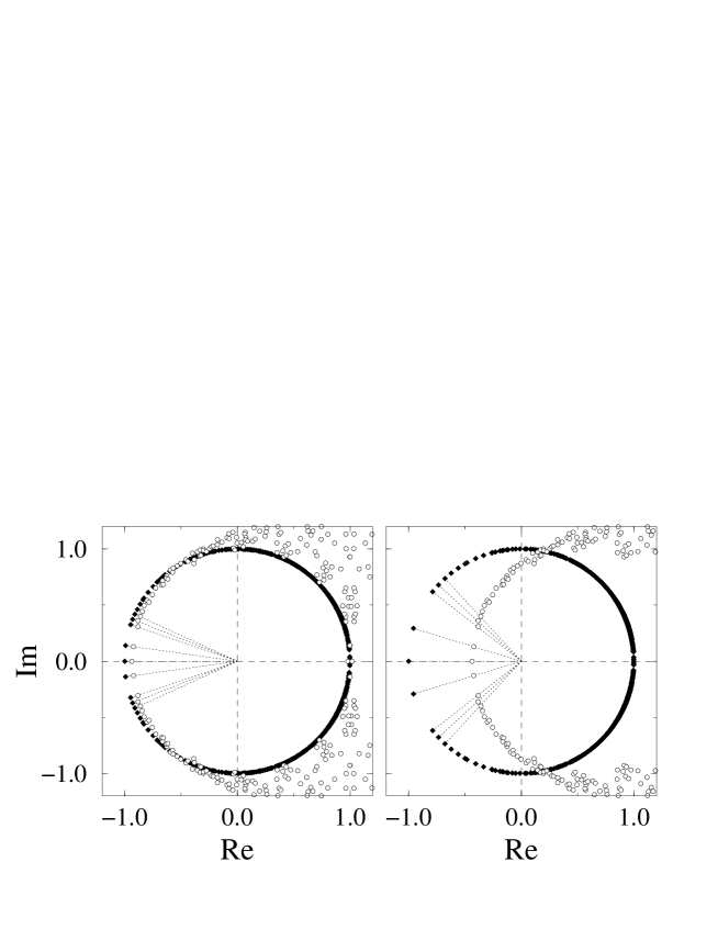
Figure 1: Eigenvalues of ${\cal D}_{\textrm{\scriptsize Wi}}\,$(open circles) and of the term $\gamma_{5}\,\epsilon(\gamma_{5}\,{\cal D}_{\textrm{\scriptsize Wi}}\,{})$ (full diamonds) in ${\cal D}_{\textrm{\scriptsize Ne}}\,$, left: $\kappa_{\textrm{\scriptsize Ne}}{}=\frac{1}{2}$, right: $\kappa_{\textrm{\scriptsize Ne}}{}=\frac{1}{3}$.

In fig. 1 we compare – for a fixed gauge configuration (at $\beta=6$) – the eigenvalues of ${\cal D}_{\textrm{\scriptsize Wi}}\,{}$ (at $\kappa=\frac{1}{2}$ and $\frac{1}{3}$; n.b. this is still above $\kappa_{c}$) with those of ${\cal D}_{\textrm{\scriptsize Ne}}\,{}-\textrm{\boldmath{$\mathsf{1}$}}=\gamma_{5}\,\epsilon(\gamma_{5}\,{\cal D}_{\textrm{\scriptsize Wi}}\,{})$ resulting from the projection (4). We find that the negative real eigenvalues of ${\cal D}_{\textrm{\scriptsize Wi}}\,$are projected to $-1$ (corresponding to $\lambda=0$): their number, counted according to the signs of their chirality, agrees with the number of zero modes of ${\cal D}_{\textrm{\scriptsize Ne}}\,$. In particular gauge configurations for smaller $\beta$ have more eigenvalues on the real axis, with a distribution density becoming broader when decreasing $\beta$. Increasing (decreasing) $\kappa_{\textrm{\scriptsize Ne}}{}$ the spectrum of ${\cal D}_{\textrm{\scriptsize Wi}}\,{}$ would shift towards left (right), and so more (less) zero modes might be obtained as a result of the projection. For small $\beta$ there is no clear distinction for ${\cal D}_{\textrm{\scriptsize Wi}}\,$between the physical branch of the real spectrum and the eigenvalues due to doubler modes. This uncertainty is discussed in the framework of the overlap method [20] and the Wilson- and Sheikholeslami-Wohlert action [21].

For ${\cal D}_{\textrm{\scriptsize Ne}}\,$, as for ${\cal D}_{\textrm{\scriptsize Wi}}\,$, not all zero modes can be equivalenced to the geometrically defined topological charge of the gauge configuration. Of course one can still define the topological charge as the number of zero modes, or equivalently the number of $\lambda=2$ modes, counting properly the chirality; in the case of the fixed point action one obtains in this way the fixed point topological charge of the lattice configuration [5]. This ambiguity vanishes towards larger $\beta$, approaching the continuum limit. Table 1 (upper part) shows the percentage $p(\beta)$ of configurations where the number of zero modes counted according to the sign of their chirality $(n_{R}-n_{L})$ (cf. the discussion in [22]) agrees with the geometric topological charge. The agreement of the first two lines is trivially explained, since the real modes counted for ${\cal D}_{\textrm{\scriptsize Wi}}\,$are those projected to $\lambda=0$ (or split into complex pairs in the case of a real pair of opposite chirality) for ${\cal D}_{\textrm{\scriptsize Ne}}\,$. This agreement stems from the choice of $\kappa_{\textrm{\scriptsize Ne}}{}$ as “cut-off” for the counting of the real modes of ${\cal D}_{\textrm{\scriptsize Wi}}\,$.

Dirac op.	$p(\beta=2)$	$p(\beta=4)$	$p(\beta=6)$
${\cal D}_{\textrm{\scriptsize Wi}}\,$	74.22	99.70	100.00
${\cal D}_{\textrm{\scriptsize Ne}}\,$	74.22	99.70	100.00
${\cal D}_{\textrm{\scriptsize Fp}}\,$	96.58	100.00	100.00
${\cal D}_{\textrm{\scriptsize Wi}}\,$	62.56	97.36	99.78
${\cal D}_{\textrm{\scriptsize Ne}}\,$	100.00	100.00	100.00
${\cal D}_{\textrm{\scriptsize Fp}}\,$	91.00	99.84	99.96

Table 1: Upper part: percentage $p(\beta)$ of configurations where the Atiyah-Singer index theorem is fulfilled. Lower part: percentage $p(\beta)$ of configurations where the vanishing theorem is fulfilled.

In table 1 (lower part) we confirm that for ${\cal D}_{\textrm{\scriptsize Ne}}\,$the zero modes have just one definite chirality, whereas for the other actions both chiralities contribute, displaying a violation of the vanishing theorem (in the case of the ${\cal D}_{\textrm{\scriptsize Fp}}\,$we believe that this violation is an effect of the truncation of less local couplings). For larger $\beta$ all three actions recover the vanishing theorem and the ASIT: $(n_{R}-n_{L})=Q_{G}$.

The density distribution of eigenvalues on (for ${\cal D}_{\textrm{\scriptsize Ne}}\,{}$) or almost on (for ${\cal D}_{\textrm{\scriptsize Fp}}\,{}$) the circle agrees with each other at small eigenvalues, with improving agreement for increasing $\beta$. For $\kappa_{\textrm{\scriptsize Ne}}{}=\frac{1}{2}$ already at $\beta=6$ the densities are indistinguishable within the statistical errors for $\mbox{Im}(\lambda)<0.6$ (Fig. 2, here we adopt the definition in [10] for the projection of the density distribution of eigenvalues to the imaginary axis). Choosing another $\kappa_{\textrm{\scriptsize Ne}}{}$ will produce another eigenvalue distribution. Comparing these with each other and with the value of $\langle\bar{\psi}\psi\rangle{}$ [11] one has to take care of the proper normalization of the fermion fields, as discussed above in sec. 2.2.

Figure 2: The unquenched eigenvalue density distribution projected from the circle onto the imaginary axis at $\beta=6$ for ${\cal D}_{\textrm{\scriptsize Fp}}\,{}$ (thick lines) and ${\cal D}_{\textrm{\scriptsize Ne}}\,{}$ with $\kappa_{\textrm{\scriptsize Ne}}{}=\frac{1}{2}$ (thin lines). The horizontal line denotes the continuum value at infinite volume.

A suitable lattice definition of $\langle\bar{\psi}\psi\rangle{}$ was suggested in the framework of the overlap action [23], which can be generalized for any fermions obeyed the GWC [24] (see [10] for an application). Also this quantity shows excellent agreement for ${\cal D}_{\textrm{\scriptsize Ne}}\,{}$ at $\kappa_{\textrm{\scriptsize Ne}}{}=\frac{1}{2}$ and ${\cal D}_{\textrm{\scriptsize Fp}}\,{}$. We obtain for the two actions (lattice units): 0.073(4) and 0.072(7) respectively for $\beta=4$, 0.062(3) and 0.063(3) for $\beta=6$ (to be compared to the continuum values 0.080 and 0.065 [25]). Choosing $\kappa_{\textrm{\scriptsize Ne}}{}=\frac{1}{3}$ with the appropriate normalization (with the factor for free fermions) we find 0.058(1) at $\beta=6$. The condensate has been studied in the 1-flavor Schwinger model in the overlap formalism already in [26], where also good agreement with the expected values has been demonstrated.

Figure 3: The dispersion relation $E(p)$ for (upper figure) the $\pi$ and (lower figure) the $\eta$ propagator for the three actions studied (lattice size $16^{2}$, $\beta=6$); squares: Wilson action, diamonds: Neuberger action, circles: fixed point action.

Discussing the mass spectrum, we find that for ${\cal D}_{\textrm{\scriptsize Ne}}\,{}$ ($\kappa_{\textrm{\scriptsize Ne}}{}=\frac{1}{2}$) the vanishing of the $\pi$-mass is excellently realized (see fig. 3); this is an amazing improvement with respect to ${\cal D}_{\textrm{\scriptsize Wi}}\,$, where the tuning to $\kappa_{c}$ creates non-irrelevant technical problems. The behavior of the energy dispersion for non-zero momenta shows no improvement compared to ${\cal D}_{\textrm{\scriptsize Wi}}\,$, while for ${\cal D}_{\textrm{\scriptsize Fp}}\,$it is almost linear as expected for a massless particle in the continuum: ${\cal D}_{\textrm{\scriptsize Fp}}\,$eliminates the cut-off effects producing a continuum-like propagator for all momenta. The massive state displays qualitatively similar behavior.

Decreasing $\kappa_{\textrm{\scriptsize Ne}}{}$ in the definition of ${\cal D}_{\textrm{\scriptsize Ne}}\,$from the suggested value $\frac{1}{2}$ down to $\frac{1}{3}$ somewhat enlarged the values of $E(p)$ slightly above those of ${\cal D}_{\textrm{\scriptsize Wi}}\,$, but still similar in the overall shape. Changing further to even smaller $\kappa_{\textrm{\scriptsize Ne}}{}$ closer to $\frac{1}{4}$ we observe, that the propagators do not reach asymptotic behavior on the lattice size studied (even for $\kappa_{\textrm{\scriptsize Ne}}{}>\kappa_{c}$) and no mass plateaus can be identified. We suspect, that this indicates larger corrections to scaling.

We also studied the correlation function (10) for the three actions. The rotational symmetry properties for ${\cal D}_{\textrm{\scriptsize Ne}}\,$are comparable to those of ${\cal D}_{\textrm{\scriptsize Wi}}\,$. Action ${\cal D}_{\textrm{\scriptsize Fp}}\,$shows the best rotational invariance. In summary, we find that the real-space correlations functions and the dispersion relations are not noticeably improved by ${\cal D}_{\textrm{\scriptsize Ne}}\,$, as compared to those for ${\cal D}_{\textrm{\scriptsize Fp}}\,$, which show a behavior substantially closer to the continuum.

It is expected that ${\cal D}_{\textrm{\scriptsize Ne}}\,$is automatically ${\cal O}(a)$ corrected [27] and thus improves scaling for the on-shell quantities; without at least introducing improvement of the current operators one would not expect improvement for the propagators as exhibited by our results.

We conclude that the identification of zero modes with the geometric topological charge for ${\cal D}_{\textrm{\scriptsize Ne}}\,$agrees with that for ${\cal D}_{\textrm{\scriptsize Wi}}\,$, if the real modes are counted according to their chirality. ${\cal D}_{\textrm{\scriptsize Fp}}\,$shows generally better behavior. The vanishing theorem, however, is satisfied automatically for ${\cal D}_{\textrm{\scriptsize Ne}}\,$, since only zero modes of one chirality result from the projection. The bound state masses and condensate come out similarly. The rotational invariance and the dispersion relations of the current propagators are not significantly improved for ${\cal D}_{\textrm{\scriptsize Ne}}\,$as compared to ${\cal D}_{\textrm{\scriptsize Wi}}\,$, but they are definitely better for ${\cal D}_{\textrm{\scriptsize Fp}}\,$.

Acknowledgment:

I.H. wishes to thank S. Chandrasekharan for a stimulating discussion and for sharing some of his unpublished results. We are grateful to W. Bietenholz and F. Niedermayer for discussions. Support by Fonds zur Förderung der Wissenschaftlichen Forschung in Österreich, Project P11502-PHY is gratefully acknowledged.

References

- [1] H. Nielsen and M. Ninomiya, Nucl. Phys. B 185 (1981) 20.
- [2] P. H. Ginsparg and K. G. Wilson, Phys. Rev. D 25 (1982) 2649.
- [3] P. Hasenfratz, Nucl. Phys. B (Proc. Suppl.) 63A-C (1997) 53.
- [4] R. Narayanan and H. Neuberger, Phys. Lett. B 302 (1993) 62; Phys. Rev. Lett. 71 (1993) 3251; Nucl. Phys. B 412 (1994) 574; ibid. B 443 (1995) 305.
- [5] P. Hasenfratz, V. Laliena, and F. Niedermayer, Phys. Lett. B 427 (1998) 125.
- [6] M. Lüscher, Phys. Lett. B 428 (1998) 342.
- [7] H. Neuberger, Phys. Lett. B 417 (1998) 141.
- [8] H. Neuberger, Phys. Lett. B 427 (1998) 353.
- [9] C. B. Lang and T. K. Pany, Nucl. Phys. B 513 (1998) 645.
- [10] F. Farchioni, C. B. Lang, and M. Wohlgenannt, Phys. Lett. B 433 (1998) 377.
- [11] T. Banks and A. Casher, Nucl. Phys. 169 (1980) 103.
- [12] S. Chandrasekharan, hep-lat/9805015.
- [13] Y. Kikukawa, R. Narayanan and H. Neuberger, Phys. Rev. D 57 (1998) 1233.
- [14] H. Neuberger, hep-lat/9806025; R. G. Edwards, U. M. Heller, and R. Narayanan, hep-lat/9807017.
- [15] T.-W. Chiu, hep-lat/9804016.
- [16] I. Hip, C. B. Lang, and R. Teppner, Nucl. Phys. (Proc. Suppl.) 63 (1998) 682.
- [17] S. Coleman, Ann. Phys. 101 (1976) 239.
- [18] C. R. Gattringer and E. Seiler, Ann. Phys. 233 (1994) 97.
- [19] J. Kiskis, Phys. Rev. D 15 (1977) 2329; N. K. Nielsen and B. Schroer, Nucl. Phys. B 127 (1977) 493; M. M. Ansourian, Phys. Lett. 70B (1977) 301.
- [20] R. G. Edwards, U. M. Heller, and R. Narayanan, hep-lat/9802016.
- [21] C. Gattringer and I. Hip, hep-lat/9806032.
- [22] P. Hernandez, hep-lat/9801035.
- [23] H. Neuberger, Phys. Rev. D 57 (1998) 5417.
- [24] P. Hasenfratz, Nucl. Phys. B525 (1998) 401.
- [25] I. Sachs and A. Wipf, Helv. Phys. Acta 65 (1992) 653.
- [26] R. Narayanan, H. Neuberger and P. Vranas, Phys. Lett. B 353 (1995) 507.
- [27] Y. Kikukawa, R. Narayanan and H. Neuberger, Phys. Lett. B 399 (1997) 105; see also: F. Niedermayer, plenary talk given at “Lattice 98”, Boulder, July 1998.