CERN-TH/98-281

NORDITA-98/56HE

hep-lat/9809004

THE ELECTROWEAK PHASE TRANSITION
IN A MAGNETIC FIELD

K. Kajantie^a,b,, M. Laine^a,b,, J. Peisa^c,, K. Rummukainen^d, and M. Shaposhnikov^a,

^aTheory Division, CERN, CH-1211 Geneva 23, Switzerland
^bDepartment of Physics, P.O.Box 9, 00014 University of Helsinki, Finland
^cDepartment of Physics, University of Wales Swansea, Singleton Park,
Swansea SA2 8PP, U.K.
^dNORDITA, Blegdamsvej 17, DK-2100 Copenhagen Ø, Denmark

Abstract

We study the finite temperature electroweak phase transition in an external hypercharge U(1) magnetic field $H_{Y}$, using lattice Monte Carlo simulations. For sufficiently small fields, $H_{Y}/T^{2}\mathop{\raise 1.29167pt\hbox{$<$\kern-7.5pt\raise-4.73611pt\hbox{$\sim$}}}0.3$, the magnetic field makes the first order transition stronger, but it still turns into a crossover for Higgs masses $m_{H}\mathop{\raise 1.29167pt\hbox{$<$\kern-7.5pt\raise-4.73611pt\hbox{$\sim$}}}80$ GeV. For larger fields, we observe a mixed phase analogous to a type I superconductor, where a single macroscopic tube of the symmetric phase, parallel to $H_{Y}$, penetrates through the broken phase. For the magnetic fields and Higgs masses studied, we did not see indications of the expected Ambjørn-Olesen phase, which should be similar to a type II superconductor.

CERN-TH/98-281
NORDITA-98/56HE
November 1998

1 Introduction

Assume that there exist non-vanishing magnetic fields in the Early Universe. Their fate then depends strongly on their scale. Long-range magnetic fields (with a scale larger than a few astronomical units today) are frozen in the primordial plasma because of its high conductivity and may survive till the present time. Magnetic fields on smaller scales dissipate by the time of recombination and seem to leave no observational trace. Thus, direct astronomical observations may put constraints on the existence of magnetic fields on cosmological distances, but cannot provide any bounds on the short-range fields. The boundary between the short-range fields (which decay by the time $t$) and the long-range fields (which still exist at time $t$) is given by the critical size $l_{0}\sim\sqrt{t/\sigma}\sim({1}/{T})\sqrt{M_{\mbox{\scriptsize Pl}}/T}$, where $\sigma\sim T$ is the plasma conductivity, $M_{\mbox{\scriptsize Pl}}$ is the Planck mass, and $T$ is the temperature of the Universe.

There were several attempts to explain the origin of the galactic magnetic fields through the creation of so-called “seed” primordial fields which may originally be weak but are amplified later through the galactic dynamo mechanism. To get a non-negligible field-strength on the galaxy scale the mechanism of magnetic field generation should be related to the inflationary stage of the Universe expansion. Generically, a whole spectrum of seed fields is produced, with an amplitude which decreases with the length-scale. Thus, it may well be that the Early Universe at temperatures higher than the electroweak scale is filled with a stochastic (hyper)magnetic field, whose contribution to the total energy density is not necessarily small at scales $\mathop{\raise 1.29167pt\hbox{$<$\kern-7.5pt\raise-4.73611pt\hbox{$\sim$}}}l_{0}$ (for a review and references see, e.g., [1]).

Potentially, strong magnetic fields may influence different processes in the Early Universe. Our primary interest here is in the electroweak phase transition, the nature of which is essential for electroweak baryogenesis. In spite of the expected stochastic and space-dependent character of the magnetic field, a constant homogeneous field approximation should be very good for this problem. Indeed, the scale of surviving magnetic fields $l_{0}\sim 10^{8}/T$ at $T\sim 100$ GeV is much greater than the typical correlation lengths.

Without any external magnetic field, the electroweak phase transition in the SU(2)$\times$U(1) Minimal Standard Model is of the first order for small Higgs masses [2]. The transition weakens with increasing $m_{H}$ so that the first order line has a second order endpoint [3] of Ising type at $m_{H,c}\approx 72$ GeV [4]. Beyond that there is only a crossover. The two phases of the system, the symmetric and the broken (or Higgs) phase, are thus analytically connected.

If there is an external magnetic field, one expects the transition to be significantly stronger [5]. This is simply because the hypercharge field $B$ contains a component of the vector field $Z$, and $Z$ acts in a way similar to the magnetic field in a superconductor: it vanishes in the broken Higgs phase. Consequently, the broken phase has an extra contribution in the free energy, and a system which would normally be considered to be deep in the broken phase can now be in coexistence with the symmetric phase, just like superconductivity can be destroyed by an external field. Numerically, one obtains in the tree approximation that for a magnetic field $H_{Y}/T_{c}^{2}\sim 0.5$, the electroweak phase transition would be of the first order and strong enough for baryogenesis up to $m_{H}\sim 160$ GeV [5]. A more precise 1-loop computation [6] (see also [7]) weakens the transition slightly: for $H_{Y}/T_{c}^{2}\sim 0.3$, one seems to be able to go up to $m_{H}\sim 100$ GeV, while for larger fields, an instability may take place.

However, finite temperature perturbation theory cannot to be trusted in the regime of large experimentally allowed Higgs masses, $m_{H}>80$ GeV. Indeed, as mentioned, the first order electroweak phase transition turns into a crossover for $m_{H}\mathop{\raise 1.29167pt\hbox{$<$\kern-7.5pt\raise-4.73611pt\hbox{$\sim$}}}80$ GeV [3, 8, 9, 4] in the absence of a magnetic field, in contrast to the perturbative prediction. Thus the effects of external magnetic fields should also be studied non-perturbatively, and this is our objective here. We do observe significant non-perturbative effects.

It is instructive to compare the present situation more precisely with a superconductor (i.e., a U(1) gauge+Higgs theory) in an external magnetic field. This system has a very rich and well studied structure. There are two possible responses to an imposed external flux:

• type I, small $m_{H}$: the flux passes through a single domain;

• type II, large $m_{H}$: the flux passes through a lattice of correlation length size vortices. In some cases, the vortex lattice can transform into a vortex liquid.

The fundamental difference between the two types is that for type II, the interface tension between bulk symmetric and broken phases is negative so that it is energetically favourable to split a single domain into a collection of small subdomains, vortices.

The physics of (hypercharge) magnetic fields in SU(2)$\times$U(1) theories has essential new features compared with superconductivity. First, the flux can now penetrate also the broken phase. Second, the broken phase massless gauge field $Q$ couples now to $W^{\pm}$ through a three-vertex, due to the non-Abelian structure of the theory. One may thus expect qualitatively new phenomena. In fact, Ambjørn and Olesen [10] have shown that for $m_{H}=m_{Z}$ the classical energy functional is minimized by a configuration containing a $W^{\pm}$-condensate with a periodic vortex-like structure. The question now is what happens in the full quantum theory.

The plan of the paper is the following. In Sec. 2 we formulate the problem in continuum, and in Sec. 3 we review briefly the perturbative estimates. In Sec. 4 we describe how the system can be put on the lattice. The numerical results are in Sec. 5 and the conclusions in Sec. 6.

2 Magnetic fields in the continuum

The theory we consider is the effective 3d theory describing the finite temperature electroweak phase transition in the Standard Model and in a part of the parameter space of the MSSM. The Lagrangian is

$$L_{\mbox{\scriptsize 3d}}={1\over 4}F_{ij}^{a}F_{ij}^{a}+{1\over 4}B_{ij}B_{ij}+(D_{i}\phi)^{\dagger}D_{i}\phi+m_{3}^{2}\phi^{\dagger}\phi+\lambda_{3}(\phi^{\dagger}\phi)^{2},$$ (1)

where $D_{i}=\partial_{i}+ig_{3}A_{i}+ig^{\prime}_{3}B_{i}/2$ and $B_{ij}=\partial_{i}B_{j}-\partial_{j}B_{i}$. The dynamics of the theory depends on the three dimensionless parameters $x$, $y$ and $z$, defined as

$$x\equiv{\lambda_{3}\over g_{3}^{2}},\qquad y\equiv{m_{3}^{2}(g_{3}^{2})\over g_{3}^{4}},\qquad z\equiv{g_{3}^{\prime 2}\over g_{3}^{2}}.$$ (2)

These parameters can be expressed in terms of the underlying physical 4d parameters and the temperature; explicit derivations have been carried out in [11, 12]. In the following, we fix $z=0.3$, corresponding to $\sin^{2}\theta_{W}=0.23$. The values $x\approx 0.10...0.13$ we have concentrated on, correspond to Higgs masses $m_{H}\approx 72...82$ GeV in the Standard Model. Moreover, $H_{Y}^{\mbox{\scriptsize 3d}}=H_{Y}^{\mbox{\scriptsize 4d}}/\sqrt{T}$ up to $O(g^{\prime 2})$ corrections which may be extracted from ref. [11] and are not important numerically. We neglect higher dimensional operators and assume that the parameters of the theory are such that this is legitimate (the relevant requirements in the absence of a magnetic field are discussed in [11]).

The external magnetic field does contribute to higher dimensional operators and thus the super-renormalizable 3d Lagrangian in Eq. (1) is not valid for arbitrarily strong magnetic fields. For instance, the 1-loop non-zero Matsubara mode contribution to the scalar mass operator in an external field is of the form $\lambda_{3}g_{3}^{\prime 2}H_{Y}^{2}\phi^{\dagger}\phi/(\pi T)^{4}$, and would give an $O(1)$ contribution to $y$ in Eq. (2) for $H_{Y}\sim(\pi T)^{2}$. Hence, one should add the condition $H_{Y}\ll(\pi T)^{2}$ to the list of requirements for the validity of dimensional reduction.

We introduce the hypercharge magnetic field with an explicitly gauge-invariant method, which can thus be easily implemented on the lattice. We consider our system in a box with periodic boundary conditions for all gauge-invariant operators. Then, the operator of the flux of the magnetic field through a surface perpendicular to the $x_{3}$-axis,

$$g_{3}^{\prime}\Phi_{B}=\int dx_{1}dx_{2}g_{3}^{\prime}B_{12}({\bf x})=g_{3}^{\prime}\oint ds_{i}B_{i}({\bf x}),$$ (3)

commutes with the Hamiltonian and is exactly conserved (the flux has been multiplied by $g_{3}^{\prime}$ to make it dimensionless also in 3d units). Thus, the equilibrium thermodynamics of the system can be described by the density matrix

$$\rho=Z^{-1}\exp(-H/T)\delta(\Phi_{B}-\Phi_{B}^{\mbox{\scriptsize cl}})$$ (4)

in the microcanonical formulation, where the value of the magnetic flux is fixed by $\Phi_{B}^{\mbox{\scriptsize cl}}$.

In the canonical formulation, the density matrix is given by

$$\rho=Z^{-1}\exp[-(H-\mu_{B}\Phi_{B})/T],$$ (5)

where $\mu_{B}$ is the “chemical potential” for the magnetic flux. In more conventional notation, $\mu_{B}$ corresponds to an external field strength $H_{Y}$, times the extent of the system in the $x_{3}$-direction, and $\Phi_{B}$ to a magnetisation density, times the area. The statistical sums in the two formulations are related, as usual, by the Legendre transformation.

It is seen from Eq. (3) that in the microcanonical formulation which we use in practice, a magnetic field can be imposed with suitable boundary conditions for $B_{i}({\bf x})$. Although $B_{i}({\bf x})$ is not itself a physical (gauge-invariant) quantity, the flux thus induced is. We stress that the local value of the (hyper)magnetic field cannot be fixed as it is not an integral of motion so that the dynamics of the system may prefer to distribute the flux of the magnetic field in an inhomogeneous way.

To discuss the physical effects of a non-vanishing flux, we shall use the following dimensionless combination:

$$b\equiv\frac{g_{3}^{\prime}}{g_{3}^{4}}B_{Y}^{\mbox{\scriptsize 3d}}\approx\frac{g^{\prime}}{g^{4}}\frac{B_{Y}^{\mbox{\scriptsize 4d}}}{T^{2}}\approx 2.0\frac{B_{Y}^{\mbox{\scriptsize 4d}}}{T^{2}},$$ (6)

where $g_{3}^{\prime}B_{Y}^{\mbox{\scriptsize 3d}}\equiv g_{3}^{\prime}\Phi_{B}/(\mbox{\rm area})$ is the magnetic flux density. For its Legendre transform,

$$H_{Y}^{\mbox{\scriptsize 3d}}=\frac{\partial f(B_{Y}^{\mbox{\scriptsize 3d}})}{\partial B_{Y}^{\mbox{\scriptsize 3d}}},$$ (7)

where $f(B_{Y}^{\mbox{\scriptsize 3d}})$ is the free energy density obtained with the density matrix in Eq. (4), we use the corresponding notation

$$h\equiv\frac{g_{3}^{\prime}}{g_{3}^{4}}H_{Y}^{\mbox{\scriptsize 3d}}.$$ (8)

The effects of $b\neq 0,h\neq 0$ can be studied in perturbation theory. There are two types of effects: First, a magnetic field gives an extra contribution to the free energy of the broken phase relative to the symmetric phase, thus changing the location of the critical curve. Second, a magnetic field affects the stability of homogeneous phases and can even lead to the emergence of completely new, inhomogeneous phases.

Figure 1: An illustration of how the electromagnetic field $Q$ in the broken phase is related to the external hypermagnetic field $B_{Y}$: $Q^{\mbox{\scriptsize actual}}=B_{Y}^{\mbox{\scriptsize input}}\cos^{-1}\theta_{W}$. $A^{3,{\mbox{\scriptsize induced}}}$ is such that the projection to the $Z$-direction vanishes.

3 The phase structure in perturbation theory

Homogeneous phases. Let us first consider the case of a fixed $b$, and assume that the ground states of the system are homogeneous. Then there is an extra free energy density related to the magnetic field. In the symmetric phase, the non-Abelian field $A^{a}_{i}$ does not have an expectation value, and the free-energy density related to gauge fields is just $B_{Y}^{2}/2$. In the broken phase, it is the electromagnetic field $Q$ which can have an expectation value, and according to Fig. 1, its contribution is $B_{Y}^{2}/(2\cos^{2}\theta_{W})$. Hence, the phase equilibrium condition for the effective potential $V(\phi,y)$ is

$$V(0,y_{c})+{\frac{1}{2}}(B_{Y}^{\mbox{\scriptsize 3d}})^{2}=V(v,y_{c})+{\frac{1}{2}}(B_{Y}^{\mbox{\scriptsize 3d}})^{2}\cos^{-2}\theta_{W},$$ (9)

where $v$ is the location of the broken minimum. It follows that for $b>0$, there is at tree-level a first order transition between homogeneous phases along the critical curve $y_{c}=-b\sqrt{2x}$, with the broken phase vacuum expectation value $v^{2}/g_{3}^{2}=b\sqrt{{2}/{x}}$.

Mixed phases. However, as is usual, one has to consider also mixed phases in addition to homogeneous phases when working with the microcanonical ensemble. A mixed phase consists of macroscopic domains of the symmetric and broken phases, and the magnetic flux can be distributed unevenly between them. Mixed phases do not appear in the canonical formulation, which thus leads to a simpler phase diagram. Let us, therefore, see what happens if the canonical variable $h$ is fixed instead of $b$.

Note first that according to Eq. (7),

$$H_{Y}^{\mbox{\scriptsize 3d}}=B_{Y}^{\mbox{\scriptsize 3d}}\quad(\mbox{symmetric phase}),\quad H_{Y}^{\mbox{\scriptsize 3d}}=B_{Y}^{\mbox{\scriptsize 3d}}\cos^{-2}\theta_{W}\quad(\mbox{broken phase}).$$ (10)

Making the Legendre transformations, the condition in Eq. (9) is replaced by

$$V(0,y_{c})-{\frac{1}{2}}(H_{Y}^{\mbox{\scriptsize 3d}})^{2}=V(v,y_{c})-{\frac{1}{2}}(H_{Y}^{\mbox{\scriptsize 3d}})^{2}\cos^{2}\theta_{W}.$$ (11)

This leads to $y_{c}=-h\sqrt{2x/(1+z)}$. One can now go back to the microcanonical ensemble, to find out that for fixed $b$, the canonical transition corresponds to a band with a finite width, $y=y_{\mbox{\scriptsize min}}...y_{\mbox{\scriptsize max}}$, where

$$y_{\mbox{\scriptsize min}}=-b\sqrt{2x}\cos^{-1}\theta_{W},\quad y_{\mbox{\scriptsize max}}=-b\sqrt{2x}\cos\theta_{W},$$ (12)

and $\cos\theta_{W}=(1+z)^{-1/2}$. Thus, the single transition line obtained from Eq. (9) splits, in fact, into two transitions between which the ground state is the mixed phase. The same result can, of course, also be obtained directly in the microcanonical formulation, by minimizing the bulk free energy of a system with certain volume fractions of the symmetric and broken phases, and an uneven distribution of the flux.

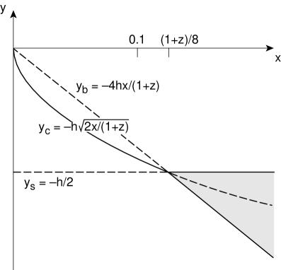
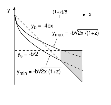
Figure 2: The tree-level phase structure in an external field. The dimensionless variables appearing are defined in Eqs. (2), (6), (8). Left: For a fixed field strength $h$, there is a first order transition along $y=y_{c}$ and an instability within the shaded region. Right: For a fixed flux density $b$, the first order transition corresponds to a band $y=y_{\mbox{\scriptsize min}}...y_{\mbox{\scriptsize max}}$ of a mixed phase.

Finally, it should be noted that a mixed phase can only appear in a large total volume $V$, when the free energy cost of the additional surfaces is less than the free energy gain obtained by going from a homogeneous phase to a mixed phase. For instance, at the point $y=-b\sqrt{2x}$, derived from Eq. (9) and lying close to the middle of the interval in Eq. (12), surfaces can only appear if

$${\frac{1}{2}}b^{2}\tan^{2}(\theta_{W}/2)(Vg_{3}^{6})>A\sigma,$$ (13)

where $A$ is the area of the surfaces, $\sigma$ is their surface tension, and $\tan^{2}(\theta_{W}/2)\approx 1/15$. For small fields, say $b\mathop{\raise 1.29167pt\hbox{$<$\kern-7.5pt\raise-4.73611pt\hbox{$\sim$}}}0.3$, and strong transitions, say $\sigma/g_{3}^{4}\mathop{\raise 1.29167pt\hbox{$>$\kern-7.5pt\raise-4.73611pt\hbox{$\sim$}}}0.3$, this requirement is satisfied if the system has a linear extension $V/A>100g_{3}^{-2}$. This distance scale is much larger than the typical correlation lengths of the system and thus quite difficult to achieve in practical lattice simulations. However, it should be remembered that even in the mixed phase, the transition takes locally always place between homogeneous phases, and these are easier to simulate.

The consideration above was at the tree-level. To estimate the magnitude of quantum corrections, one may compute how $H_{Y}$ affects the $W^{\pm},Z^{0}$ loop contributions in the broken phase free energy. At 1-loop level, the answer is

$$V_{W^{\pm},Z^{0}}^{\rm 1-loop}(v,y_{c}) = -{1\over 12\pi}(4m_{W}^{3}+2m_{Z}^{3})-{e_{3}Q\over 2\pi}(\sqrt{m_{W}^{2}+e_{3}Q}-\sqrt{m_{W}^{2}-e_{3}Q})$$ (14)

$$+{1\over 4\pi^{3/2}}\int_{0}^{\infty}{dt\over t^{3/2}}e^{-m_{W}^{2}t}\left({1\over t}-{e_{3}Q\over\sinh e_{3}Qt}\right),$$

where $m_{W}={\frac{1}{2}}gv,m_{Z}=m_{W}\sqrt{1+z}$, and $e_{3}Q=g_{3}^{\prime}B_{Y}$. Eq. (14) can be reliably converted to a 1-loop change in $y_{c}$ if the correction is smaller than the leading magnetic energy term following from Eq. (11): this requires that $h\mathop{\raise 1.29167pt\hbox{$>$\kern-7.5pt\raise-4.73611pt\hbox{$\sim$}}}0.15$ and that $x$ not be too small, $1/(2\pi\sqrt{h})\ll(8x)^{3/4}$. Then,

$$y_{c}^{\mbox{\scriptsize 1-loop}}(x,h)=-h\sqrt{\frac{2x}{1+z}}+\frac{\sqrt{h}}{4\pi(8x(1+z))^{{\frac{1}{4}}}}\biggl{[}{\frac{2}{3}}+{(1+z)^{{\frac{3}{2}}}\over 3}$$ (15)

$$+(\frac{8x}{1+z})^{{\frac{1}{2}}}\Bigl{(}\sqrt{1+(\frac{8x}{1+z})^{{\frac{1}{2}}}}-\sqrt{1-(\frac{8x}{1+z})^{{\frac{1}{2}}}}\Bigr{)}-\frac{2x}{3(1+z)}\Bigl{(}1-\frac{7}{10}\frac{x}{1+z}+{\cal O}(x^{2})\Bigr{)}\biggr{]}.$$

Qualitatively, the effect of 1-loop corrections is that the regime $x>(1+z)/8$ becomes unstable (has an imaginary part), and that the value of $y_{c}$ is somewhat less negative than at tree-level.

The stability of the homogeneous phases. According to the standard Landau-level analysis, the effective mass squared of the Higgs field in the symmetric phase is modified by the term $+(g_{3}^{\prime}/2)B_{Y}^{\mbox{\scriptsize 3d}}$ in the presence of a magnetic field, while the vector mass squared remains zero. In the broken phase, in contrast, the neutral Higgs mass squared remains unmodified, while the $W^{\pm}$-bosons get a term $-e_{3}Q=-g_{3}^{\prime}B_{Y}^{\mbox{\scriptsize 3d}}$. This term is characteristic of non-Abelian gauge theories. For a stable phase, the mass squared must be positive. Thus we get that the symmetric phase is stable at

$$y>y_{s}=-h/2,$$ (16)

while the broken phase is stable at

$$y<y_{b}=-4hx/(1+z).$$ (17)

For $y_{s}>y_{b}$, which can happen when $x>(1+z)/8$, neither phase is stable. Therefore, in this region of the parameter space the ground state of the system must be inhomogeneous. In a superconductor, an external magnetic field cannot penetrate the broken Higgs phase, and the flux goes either through a macroscopic tube of the symmetric phase (type I superconductors) or through a vortex lattice (type II superconductors). In the present case, the magnetic field can penetrate the broken phase. Nevertheless, a behaviour similar to a type I or type II superconductor can emerge. As we have seen, a type I mixed phase behaviour appears on the first order line shown in Fig. 2, for $x<(1+z)/8$. The relevant ground state in the regime $x>(1+z)/8,y_{s}>y_{b}$ has been studied by Ambjørn and Olesen (AO) [10]. It contains a $W^{\pm}$-condensate, with a periodic vortex-like structure, similar to a type II superconductor. The emerging tree-level phase structure is illustrated in Fig. 2.

Our main aim below is to analyse numerically if this phase structure is stable against quantum fluctuations.

4 Magnetic fields on the lattice

The theory in Eq. (1) can be discretized in the standard way (see, e.g., [2]). The lattice action is

$$S = \beta_{G}\sum_{x}\sum_{i<j}[1-{\frac{1}{2}}{\rm Tr\,}P_{ij}]+{\frac{1}{2}}\frac{\beta_{G}}{z}\sum_{x}\sum_{i<j}\alpha_{ij}^{2}$$ (18)

$$- \beta_{H}\sum_{x}\sum_{i}{\frac{1}{2}}{\rm Tr\,}\Phi^{\dagger}(x)U_{i}(x)\Phi(x+i)e^{-i\alpha_{i}(x)\sigma_{3}}$$

$$+ \beta_{2}\sum_{x}{\frac{1}{2}}{\rm Tr\,}\Phi^{\dagger}(x)\Phi(x)+\beta_{4}\sum_{x}\bigl{[}{\frac{1}{2}}{\rm Tr\,}\Phi^{\dagger}(x)\Phi(x)\bigr{]}^{2},$$

where $\alpha_{i}=a(g_{3}^{\prime}/2)B_{i}$, $\alpha_{ij}(x)=\alpha_{i}(x)+\alpha_{j}(x+i)-\alpha_{i}(x+j)-\alpha_{j}(x)$ is the discretized field strength tensor, and $\Phi=(i\tau^{2}\phi^{*},\phi)$. The dimensionless lattice field is $\phi^{\dagger}\phi_{\mbox{\scriptsize latt}}=\phi^{\dagger}\phi_{\mbox{\scriptsize cont}}/g_{3}^{2}$, and the couplings are

$$\beta_{G}=\frac{4}{ag_{3}^{2}},\quad\beta_{H}=\frac{8}{\beta_{G}},\quad\beta_{2}=\frac{24}{\beta_{G}}+\frac{64}{\beta_{G}^{3}}\frac{m^{2}}{g_{3}^{4}},\quad\beta_{4}=\frac{64}{\beta_{G}^{3}}x,$$ (19)

where $m^{2}$ can be read from Eq. (33) in [13], with $\gamma=\infty$. In this paper, we use only one value of $\beta_{G}$, $\beta_{G}=8$, since we monitor mainly shifts in quantities whose discretization errors are already known from simulations without a magnetic field.

On a lattice with the extent $N_{1}N_{2}N_{3}$, the flux of Eq. (3) to the $x_{3}$-direction is imposed by modifying the periodic boundary conditions of the variables $\alpha_{i}$ as follows (for each fixed $n_{3}$ in $\alpha_{i}(n_{1},n_{2},n_{3})$, not written explicitly):

$$g_{3}^{\prime}\Phi_{B}=2\Bigl{\{}\sum_{n_{1}=1}^{N_{1}}\Bigl{[}\alpha_{1}(n_{1},0)-\alpha_{1}(n_{1},N_{2})\Bigr{]}+\sum_{n_{2}=1}^{N_{2}}\Bigl{[}\alpha_{2}(N_{1},n_{2})-\alpha_{2}(0,n_{2})\Bigr{]}\Bigr{\}}.$$ (20)

With strictly periodic boundaries for $\alpha_{i}$, the net flux is thus zero.

In principle, any flux $\Phi_{B}$ can be simulated. However, the action is not periodic unless the quantities in the square brackets in Eq. (20) are integer multiples of $2\pi$. The violation of these conditions will result in boundary defects (boundary currents), and the lattice translational invariance will be lost. This requirement quantizes the total flux: $g^{\prime}_{3}\Phi_{B}/2=2\pi n$, with $n$ an integer.

The most economical way of implementing the boundary conditions is to make only one $(x,y)$-plane link aperiodic. Thus, the boundary condition in Eq. (20) becomes

$$\alpha_{1}(n_{1},0)-\alpha_{1}(n_{1},N_{2})=2n\pi\delta_{n_{1},1}\,,$$ (21)

otherwise $\alpha_{i}$ periodic. Despite its appearance, this condition does not give any special physical status to the $n_{1}=1$ -plane, or the $x$-direction, since the ‘twist’ can be transformed to an arbitrary location without modifying the action.

It is essential that in Eq. (18) the hypercharge field $\alpha_{i}$ has a non-compact action. For a compact action the variables $\alpha_{i}$ are only defined modulo $2\pi$, and the boundary conditions above reduce to purely periodic ones. In this case the flux can spontaneously fluctuate in units of $2\pi$ from configuration to configuration, and the mean flux will average to zero.

In terms of the flux density parameter $B_{Y}^{\mbox{\scriptsize 3d}}$ appearing in Eq. (6), the quantization condition is $a^{2}N_{1}N_{2}(g_{3}^{\prime}/2)B_{Y}^{\mbox{\scriptsize 3d}}=2\pi n$, and the dimensionless variable $b$ characterizing the average magnetic flux density is then

$$b=\frac{g_{3}^{\prime}B_{Y}^{\mbox{\scriptsize 3d}}}{g_{3}^{4}}=\Bigl{(}\frac{\beta_{G}}{4}\Bigr{)}^{2}\frac{4\pi n}{N_{1}N_{2}}.$$ (22)

As to the observables measured, let us mention that in addition to the usual volume averages of gauge-invariant operators, it is useful to study gauge-invariant operators summed over the $x_{3}$-direction, and only a small sub-block of the $(x_{1},x_{2})$-plane:

$$(\phi^{\dagger}\phi)_{\mbox{\scriptsize blocked}}=\sum_{n_{3}=1}^{N_{3}}\sum_{(n_{1},n_{2})\in{\mbox{\scriptsize block}}}\phi^{\dagger}\phi(n_{1},n_{2},n_{3}).$$ (23)

The distribution of such observables is sensitive to possible inhomogeneous spatial structures.

5 Results

We have performed Monte Carlo simulations with $x$ in the range $0.1\leq x\leq 0.2$ and a magnetic field in the range $0\leq b\leq 24\pi/64$, with volumes up to $64^{3}$ (Table 1). The total number of runs (combinations of volumes and couplings $(x,y,b)$) is 548. As mentioned in connection with Eq. (13), it should be kept in mind, though, that the true infinite volume limit is impossible to achieve in some regions of the parameter space.

$x$	$b/(\pi/64)$	volumes
0.10	0, 4, 8, 12	$16^{3}$, $22^{3}$, $28^{3}$, $32^{3}$
0.11	24	$32^{3}$
0.12	0, 8, 16, 24	$16^{3}$, $32^{3}$
0.121	16	$48^{3}$
0.125	24	$16^{3}$, $32^{3}$, $48^{3}$
0.13	0, 8, 16, 24	$16^{3}$, $32^{3}$
0.14	24	$32^{3}$
0.15	0, 8, 16, 24	$16^{3}$
0.16	24	$32^{3}$, $64^{3}$
0.20	0, 8, 16	$16^{3}$, $32^{3}$

Table 1: The simulation points at fixed $x$. In each case, several values of $y$ (up to 20) were used. Extensive additional simulations were performed close to the endpoints of the first order transition lines for $b/(\pi/64)=1$,2,3,4,6,12,16,24 (see Fig. 4). All the simulations reported here are with $\beta_{G}=8$. For the volumes $22^{3}$ and $28^{3}$ the closest approximation to the $b$ indicated, satisfying the quantization rule in Eq. (22), was used.

Figure 3: The probability distribution of $\phi^{\dagger}\phi$ at $x=0.1$ and $y=y_{c}$, measured with four different flux densities and the volumes $16^{3}$ and $32^{3}$. The transition becomes stronger (the separation of the peaks increases and the probability between the peaks decreases) and $y_{c}$ decreases with increasing $b$. Simulations with $b\geq 4\pi/64$ are multicanonical. For the cubic geometry employed, the “mixed” configurations where the volume average of $\phi^{\dagger}\phi$ is between the two peaks, prefer to have phase interfaces parallel with the magnetic field. For much larger volumes, a single peak corresponding to the mixed phase would appear in between the two peaks seen here, see Fig. 7.

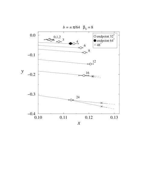
Figure 4: The $0.10<x<0.13$ part of the phase diagrams for constant $b$, $0\leq b\leq 24\pi/64$, and finite volumes. The continuous lines show first order phase transitions (for clarity, not shown for $n<4$), and the open and filled circles the endpoint/triple point locations. At large fields ($n\geq 16$) a ‘type I’ mixed phase appears between the symmetric and broken phases. The transitions have been located on the points shown with the crosses. All the transitions become weaker when $x$ increases. The behaviour at large $x$ is not known (dashed lines), but we expect the region opening at the triple point to be closed. When the lattice size is increased, the triple points appear at smaller $x$ and $b$.

Small fields.

For $b=0$, the line of first order phase transitions at small $x$ has an endpoint, in the universality class of the Ising model [4]. According to the discussion in Sec. 3, for $b\neq 0$ the transition line should split into two lines with a mixed phase in between. However, we find that for small $b$ the mixed phase remains absent for all practical lattice sizes (see Eq. (13)). Indeed, we observe that the $b=0$ qualitative behaviour remains there for small $b$, even though the endpoint moves to larger $x$. Moreover, for any given $x<x_{c}$ (the endpoint location at $b=0$), the transition becomes more strongly of the first order for increasing $b$. This is shown in Fig. 3 for $x=0.1$.

We have determined the finite volume endpoint location with a method similar to that used in [4]: for each $b$, we locate the point $(x_{c},y_{c})$ where the order parameter probability histogram $P(\phi^{\dagger}\phi)$ has two peaks of equal height, and the peaks are approximately 2.2 times higher than the histogram height between the peaks, a characteristic value for the magnetization distribution of the 3d Ising model at the critical point. As an example, the $b=0$ histogram shown in Fig. 3 almost fulfills this criterion for $(x_{c},y_{c})$. (The main deviation comes from the fact that in Fig. 3 the values of $y_{c}$ have been determined by the more common equal weight  criterion. However, the equal height method is better suited for searching for the endpoint location.)

The actual process of locating the critical point consists of two stages: First, a few short simulations are performed near the estimated critical point, giving a series of improved estimates. Then, a long simulation is performed using the best estimate for the critical point. Finally, the resulting probability histogram $P(\phi^{\dagger}\phi)$ is reweighted  with respect to $x$ and $y$ until the critical point condition mentioned above is fulfilled, which yields the final value of $(x_{c},y_{c})$. For details of this procedure we refer to [4].

The results, together with the critical lines, are shown in Fig. 4. The main observation is that $x_{c}$ increases quite slowly with $b$, and does not reach values larger than $\sim 0.125$ for $b\mathop{\raise 1.29167pt\hbox{$<$\kern-7.5pt\raise-4.73611pt\hbox{$\sim$}}}1$. We have used mostly $\beta_{G}=8$, volume $=32^{3}$ lattices for this analysis. Strictly speaking, the situation is slightly more complicated in the infinite volume limit because of the appearance of the mixed phase. Nevertheless, the finite volume results are indicative of the shift  of the transition line and $(x_{c},y_{c})$ as functions of $b$. Indeed, the location of the endpoint does not change significantly when the volume is increased from $32^{3}$ to $64^{3}$ at $b=4\pi/64$; see Fig. 4.

   

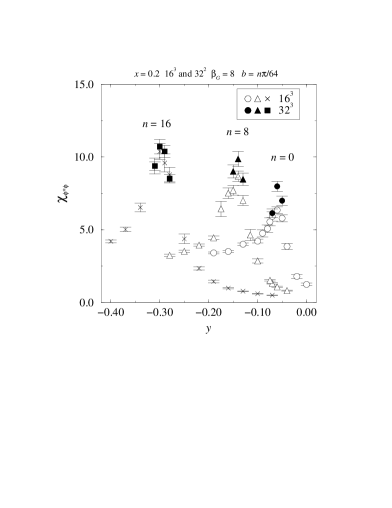
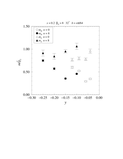
Figure 5: The crossover region at $x=0.2$ for $b\leq 16\pi/64$. Left: The $\phi^{\dagger}\phi$ susceptibility. While the susceptibility has a clear peak at the crossover, it does not diverge when the volume is increased. Right: The inverse correlation lengths. In contrast with perturbation theory, there is always a non-vanishing mass, and thus no 2nd order phase transition. The photon mass vanishes everywhere.

Searching for the Ambjørn–Olesen phase.

According to the tree-level structure in Fig. 2, there should be an inhomogeneous Ambjørn–Olesen (AO) phase at large Higgs masses, $x>(1+z)/8$. In this phase $\phi^{\dagger}\phi$ has a non-zero expectation value with a periodic spatial structure in analogy with vortices in type II superconductors, and there is a $W^{\pm}$-condensate.

Indeed, we do  observe the AO phase in classical configurations (which are solutions of the lattice equations of motion): if we take a lattice configuration at $x>(1+z)/8$, $y\sim-b\sqrt{2x}$ (see Eq. (12)), and ‘cool’ it so that it minimizes the lattice action in Eq. (18), a periodic $\phi$ and $W$ structure emerges. However, the ‘quantum’ configurations (which contribute to the lattice partition function) contain a lot of fluctuations, and it is far from straightforward to observe whether there is an underlying structure in them.

The cooling mentioned proceeds very much like the standard lattice Monte Carlo update, but instead of a new thermally distributed value, the field variables are chosen so that the local action is minimized. In one cooling sweep the action is minimized at each lattice point and for all of the lattice fields. The UV noise vanishes after only a few cooling sweeps, but cooling down to the classical configuration can take several thousands of update sweeps.

Using the standard global thermodynamic quantities on the lattice, on the other hand, we do not observe any transition to a phase with qualitatively new properties at $x=0.2$. The behaviour of the $\phi^{\dagger}\phi$ susceptibility $\chi_{\phi^{\dagger}\phi}=V\langle(\phi^{\dagger}\phi-\langle\phi^{\dagger}\phi\rangle)^{2}\rangle$ is shown in Fig. 5(left), and the behaviour does not change qualitatively from that at $b=0$.

It is also possible to directly try to measure the $W^{+}W^{-}$-condensate on the lattice. For example, the (lattice) operator $W^{+}_{1}W^{-}_{2}-W^{+}_{2}W^{-}_{1}$ is gauge invariant and, in the absence of an external magnetic field, has a vanishing expectation value. However, when there is an external field in the $x_{3}$-direction, this operator acquires a non-zero expectation value, even deep in the symmetric and broken phases where there is no $W^{+}W^{-}$-condensate. While we do observe a clear increase of the condensate operator in the crossover region, a similar increase is also seen near the first order transition. Thus, we cannot assign this increase to the appearance of a $W^{+}W^{-}$-condensate.

A clear signature of the AO phase is its periodic spatial structure in the $(x_{1},x_{2})$-plane (or, if the strict periodicity is destroyed by fluctuations, there should at least be an enhancement of the characteristic wavelengths of the lattice fields). We have attempted to directly observe this on the lattice at $x=0.2$, $b\leq 16\pi/64$ with various methods:

• A moderate amount of cooling is a very efficient method of getting rid of the lattice UV noise. However, in this case the interpretation of the results is far from clear: if we cool the configuration too much, it will be driven towards the solution of the classical equations of motion and finally reveal the structure of the AO phase. To deem the ‘correct’ amount of cooling is ambiguous, at best. It is much more objective to measure the properties of configurations without any cooling.

• The Fourier power spectrum of $\phi^{\dagger}\phi$ in the $(x_{1},x_{2})$-plane should reveal the presence of periodic spatial structures. However, in our measurements the spectrum remains qualitatively the same for both $b=0$ and $b\neq 0$.

• Since the AO field structure is of classical nature, it should persist on the lattice for several update cycles, whereas the quantum noise rapidly averages to zero. This can be utilized by averaging the fields over a various number of consecutive configurations (and over the $x_{3}$-direction). However, this analysis does not reveal any non-trivial structure.

• All polarizations of the photon, in all directions, remain massless.

We thus have to conclude that small magnetic fields do not result in an inhomogeneous phase at around $x=0.2$. A possible explanation is that, in contrast to tree-level perturbation theory, the non-perturbative inverse correlation lengths are always non-vanishing in this regime, as shown in Fig. 5(right). Thus there may be some minimum value of $b$ which is needed for the instability and the inhomogeneous phase to appear.

Figure 6: A Higgs field configuration on a $48^{3}$ lattice for $x=0.125$, $y=-0.36$, just above the transition to the broken homogeneous phase. A thermodynamically stable  cylinder of the symmetric phase is surrounded by the broken phase. In order to reduce noise in the plot, we have cooled the configuration with 10 local cooling sweeps, and averaged the fields over the $x_{3}$-direction.

Figure 7: The appearance of the ‘type I’ mixed phase at $b=24\pi/64$. Top: The $\phi^{\dagger}\phi$ histogram measured at the triple point, where the symmetric phase (left peak), broken phase (right peak) and the mixed phase (center) coexist. Strong first order transitions separate the phases at this finite volume. A dashed line shows the distribution of the blocked $\phi^{\dagger}\phi$ in the mixed phase, measured over $1/16$th of the total area (see Eq. (23)). Here the center peak is absent, in accord with the mixed broken/symmetric spatial structure of the mixed phase. Bottom: The global $\phi^{\dagger}\phi$ histograms at $x=0.125$, $V=48^{3}$. Separate first order transitions occur at $y\approx-0.346$ and $y\approx-0.3626$; for intermediate values of $y$ the mixed phase is stable.

Large fields.

For large values of the magnetic field we do observe a mixed phase. This phase consists of a domain of the symmetric phase surrounded by the broken phase. A moderately cooled Higgs field configuration is shown in Fig. 6, for $x=0.125$, $y=-0.36$, and $b=24\pi/64$. Inside the symmetric phase domain, the hypermagnetic field is somewhat ($\sim 25\%$) larger than elsewhere. For the Higgs field, the behaviour is similar to that in a type I superconductor, and we shall thus use the name “type I” for this mixed phase.

For each lattice size and (large enough) $b$, the type I phase appears only in some specific interval of $x$: if $x$ is too small, the first order nature of the symmetric $\leftrightarrow$ broken transition is too strong for the mixed phase to appear in the volumes we can simulate in practice. This is due to the tension (free energy density) of the interface between the symmetric and broken domains in the mixed phase. At a triple point  $(x,y)_{\rm triple}$, the symmetric, broken and mixed phases are equally likely to appear. This is illustrated in the top part of Fig. 7. The transitions separating the three phases are of the first order. When $x$ is further increased, separate symmetric $\leftrightarrow$ type I and type I $\leftrightarrow$ broken transitions appear. This is shown in the bottom part of Fig. 7.

The resulting phase diagrams are shown in Fig. 4. When $x>x_{\rm triple}$, a band of the type I phase appears, separated by lines of first order transitions. For each fixed $(x,y)$, the type I mixed phase contains a definite volume fraction of the symmetric phase (by a volume fraction we mean the weight of the corresponding peak in the local ’blocked’ distribution, see Fig. 7). At the upper (lower) critical $y_{c}(x)$, the symmetric phase occupies the largest (smallest) volume fraction. At the triple point these limits are equal. For a finite total volume, it is not possible to have a mixed phase with arbitrary volume fractions.

When the volume is increased, the interface tension becomes less significant in comparison with the bulk free energies. Thus, when the volume goes to infinity, $x_{\rm triple}\rightarrow 0$, and the mixed phase band becomes slightly wider (since now it is possible to have arbitrary volume fractions). However, the simulations near the triple point are very difficult, and we have not attempted to study the volume dependence of $x_{\rm triple}$ in detail.

The first order transitions separating the homogeneous phases from the mixed phase become weaker when $x$ increases. At $x\approx 0.2$ we have not observed transitions any more, and symmetric and broken phases appear to be analytically connected. However, since the type I phase breaks translational invariance (in the sense that after the removal of a zero mode, the observables measured depend on the location), it has to be separated from the symmetric and broken phases by some kind of phase transitions. Thus, the type I regions in Fig. 4 should form isolated domains, or they could also transform into an AO phase at some $x$.

Finally, a couple of technical issues about the phase structure on the lattice:

First, the locations of the transitions between the type I and the homogeneous phases are very sensitive to finite size effects. The volume should be large enough in order for the phase interfaces in the mixed phase to have a negligible effect. This is very difficult to achieve in practice. In Fig. 4 the transitions have been located with a $48^{3}$ lattice; using a larger volume would widen the type I region, and move the triple point to smaller $x$.

Second, on a periodic toroidal lattice there are also two other transitions besides the ones shown in Figs. 4, 7: these correspond to transitions where a cylindrical domain (Fig. 6) becomes a slab spanning the lattice in $(x_{1},x_{3})$ or $(x_{2},x_{3})$-directions. These transitions are not physical, since they are caused by the boundary conditions.

6 Conclusions

We have found that for Higgs mass $m_{H}\mathop{\raise 1.29167pt\hbox{$>$\kern-7.5pt\raise-4.73611pt\hbox{$\sim$}}}80$ GeV, even magnetic fields up to $H_{Y}/T^{2}\sim 0.3$ ($b\sim 0.6$) do not suffice to make the transition be of the first order: there is only a crossover. This is in contrast to the perturbative estimates in [5, 6]. Moreover, we do not observe any sign of the exotic phase with broken translational invariance proposed by Ambjørn and Olesen for these magnetic fields: all the gauge-invariant operators and correlation lengths we have studied behave qualitatively as without a magnetic field, even though the solution of the classical equations of motion has a vortex structure with a $W^{\pm}$-condensate. We conclude that fluctuations are strong enough to remove the non-trivial structure for the parameter values studied.

On the other hand, for the finite volumes studied, we do observe the emergence of a new phase when the magnetic field is increased above $H_{Y}/T^{2}\sim 0.3$. This phase is not of the type proposed by Ambjørn and Olesen, though, but it is a mixed phase, with a Higgs field distribution similar to a type I superconductor. It would be interesting to determine whether this phase turns into the Ambjørn-Olesen phase at larger Higgs masses. We expect that the phases with broken translational invariance (i.e., type I and AO), appear in a closed region of the parameter space, terminating at some $x_{c}$. The fact that the transition terminates also at a non-vanishing magnetic field, is a non-perturbative phenomenon and does not appear in the tree-level phase diagram in Fig. 2. A more precise study of these questions is in progress.

The implications of a magnetically stabilized mixed phase structure on different scenarios of electroweak baryogenesis have, to our knowledge, not been studied before, but there might be some effects. A precise investigation of these issues is beyond the scope of the present paper.

References

- [1] K. Enqvist, Int. J. Mod. Phys. D 7 (1998) 331 [astro-ph/9803196].
- [2] K. Kajantie, M. Laine, K. Rummukainen and M. Shaposhnikov, Nucl. Phys. B 493 (1997) 413 [hep-lat/9612006].
- [3] K. Kajantie, M. Laine, K. Rummukainen and M. Shaposhnikov, Phys. Rev. Lett. 77 (1996) 2887 [hep-ph/9605288].
- [4] K. Rummukainen, M. Tsypin, K. Kajantie, M. Laine and M. Shaposhnikov, Nucl. Phys. B 532 (1998) 283 [hep-lat/9805013].
- [5] M. Giovannini and M.E. Shaposhnikov, Phys. Rev. D 57 (1998) 2186 [hep-ph/9710234].
- [6] P. Elmfors, K. Enqvist and K. Kainulainen, HIP-1998-31-TH [hep-ph/9806403].
- [7] A.S. Vshivtsev, V.Ch. Zhukovsky and A.O. Starinets, Z. Phys. C 61 (1994) 285; V. Skalozub and M. Bordag, hep-ph/9807510.
- [8] F. Karsch, T. Neuhaus, A. Patkós and J. Rank, Nucl. Phys. B (Proc. Suppl.) 53 (1997) 623 [hep-lat/9608087].
- [9] M. Gürtler, E.-M. Ilgenfritz and A. Schiller, Phys. Rev. D 56 (1997) 3888 [hep-lat/9704013].
- [10] J. Ambjørn and P. Olesen, Nucl. Phys. B 315 (1989) 606; Phys. Lett. B 218 (1989) 67; Nucl. Phys. B 330 (1990) 193; Int. J. Mod. Phys. A 5 (1990) 4525.
- [11] K. Kajantie, M. Laine, K. Rummukainen and M. Shaposhnikov, Nucl. Phys. B 458 (1996) 90 [hep-ph/9508379]; Phys. Lett. B 423 (1998) 137 [hep-ph/9710538].
- [12] M. Laine, Nucl. Phys. B 481 (1996) 43 [hep-ph/9605283]; J.M. Cline and K. Kainulainen, Nucl. Phys. B 482 (1996) 73 [hep-ph/9605235]; Nucl. Phys. B 510 (1997) 88 [hep-ph/9705201]; M. Losada, Phys. Rev. D 56 (1997) 2893 [hep-ph/9605266]; G.R. Farrar and M. Losada, Phys. Lett. B 406 (1997) 60 [hep-ph/9612346].
- [13] M. Laine and A. Rajantie, Nucl. Phys. B 513 (1998) 471 [hep-lat/9705003].